Natural Convection in a Non-Newtonian Fluid: Effects of Particle Concentration


1
University of Florida, Engineering School of Sustainable Infrastructure and Environment, Gainesville, FL 32611, USA
2
School of Mechanical Engineering, Nanjing University of Science and Technology, Nanjing 210094, China
3
U.S. Department of Energy, National Energy Technology Laboratory (NETL), Pittsburgh, PA 15236, USA
*
Author to whom correspondence should be addressed.
Fluids 2019, 4(4), 192; https://doi.org/10.3390/fluids4040192
Submission received: 1 October 2019
/
Revised: 17 October 2019
/
Accepted: 23 October 2019
/
Published: 1 November 2019
(This article belongs to the Special Issue Recent Advances in Mechanics of Non-Newtonian Fluids)
Abstract
:In this paper we study the buoyancy driven flow of a particulate suspension between two inclined walls. The suspension is modeled as a non-linear fluid, where the (shear) viscosity depends on the concentration (volume fraction of particles) and the shear rate. The motion of the particles is determined by a convection-diffusion equation. The equations are made dimensionless and the boundary value problem is solved numerically. A parametric study is performed, and velocity, concentration and temperature profiles are obtained for various values of the dimensionless numbers. The numerical results indicate that due to the non-uniform shear rate, the particles tend to concentrate near the centerline; however, for a small Lewis number (Le) related to the size of the particles, a uniform concentration distribution can be achieved.
1. Introduction
Fluid flow can occur for various reasons such as applications of external forces, presence of pressure or temperature gradients, natural convection (buoyancy driven flow), etc. The latter type is when the density of the fluid is a function of temperature and as a result due to a temperature dependent buoyancy (body) force the fluid can move (see Turner (1979) [1]). Natural convection and heat transfer in a suspension composed of solid particles and a fluid occur in thermal storage systems, chemical industry or food industry [2,3]. Studying the natural convection and flow of suspensions can provide better understanding of the complex mechanisms involved in these flows [4,5]. Particulate suspensions usually show some of the non-Newtonian features, such as shear-thinning, yield stress, thixotropy, dilatancy, normal stress effects, and even anisotropic thermal or momentum diffusivity. Metivier et al. (2017) [6] experimentally studied the onset of the Rayleigh-Bénard convection of a concentrated suspension of microgels subject to a temperature gradient. They focused their studies on the no-slip condition and found that the main control parameters for this flow is the ratio between the yield stress and the buoyancy force. Sun et al. (2019) [3] investigated the natural convection and heat transfer of a ferro-nanofluid with anisotropic thermal conductivity under a magnetic field. The numerical results show that the isotherms become elliptic and deviate from the circular pattern which is the typical pattern with isotropic thermal conductivity.
In general, due to certain effects such as the presence of lift force or drag force, the suspension can exhibit certain multi-component features, such as particle migration or particle sedimentation; moreover, in many situations, due to the presence of gravity or some other body forces (such as electro-magnetic forces) the solid particles can redistribute themselves and cause a change in the rheological properties of the suspension. Okada and Suzuki (1997) [7] experimentally investigated the natural convection of particulate suspension in a rectangular cell where the central part of the lower wall was heated. They found that the suspension forms different layers during the sedimentation of particles, and these layers disappear as the flow evolves; they attributed this phenomenon to the double diffusive convection caused by the volume fraction and the temperature gradient. Using Particle Tracking Velocimetry (PTV), Chen et al. (2005) [2] measured the velocity and the particle distributions in a square section with the bottom wall heated; they noticed that the flow patterns of the particulate suspension, such as sedimentation driven convection, is distinct from the flow of fluid with no particles.
Natural convection problems related to meteorology (see Batchelor (1954) [8]) and non-Newtonian fluids have been studied extensively (see Shenoy and Mashelkar (1982) [9]). For example, Rajagopal and Na (1985) [10] studied the natural convection of grade fluids between two vertical walls. Massoudi and Christie (1990) [11] considered the flow due to natural convection of a thermodynamically compatible third grade fluid between two vertical cylinders. Later, Massoudi et al. (2008) [12] studied the natural convection of a generalized second grade fluid with a temperature dependent and shear-rate dependent viscosity. In these studies, the fluid was not considered to be a suspension of particles in a fluid and as a result the effect of volume fraction was ignored.
In this paper we do consider the effect of volume fraction of the particles and we will look at the buoyancy driven flow of a particulate suspension between two inclined walls with variable transport properties. In Section 2 and Section 3 we present the governing equations and the constitutive relations, respectively. In Section 4, we look at the simplified equations for the natural convection flow and present the governing equations and the boundary conditions along with our assumptions. In Section 5, the results are analyzed. Finally, in Section 6 we present the conclusions.
2. Governing Equations
As mentioned earlier, in general, most suspensions behave as multi-component fluids. They can be modeled using the techniques of suspension rheology or the techniques of multi-component materials (mixture theory). While the former method is easier to handle computationally (fewer equations), it also has the disadvantage that it cannot predict many of the interesting phenomena observed in multicomponent flows, such as the various possible interactions between different components, such as lift forces, drag forces, etc. For example, for a two-component system, the governing equations are written for each component (phase) and constitutive relations are needed for the two stress tensors, the interaction forces, the flux vectors, etc. Clearly, this approach, while more accurate, will be computationally more intensive. For a recent discussion of the multi-component approach we refer the reader to Rajagopal and Tao (1995) [13]; Massoudi (2003, 2008, 2010) [14,15,16]. As a compromise, one can look at the suspension which does have some type of structure (in this case solid particles which can be re-arranged and move with the velocity of the suspension), as a single component non-linear fluid, allowing for the presence of the particles through the introduction of a concentration (volume fraction) field . In this paper, we take this approach and model the suspension as a (single component) non-linear fluid; in this case the governing equations of motion are the conservation of mass, linear and angular momentum, and the energy equations. These equations are (see for example, Slattery (1999) [17]):
2.1. Conservation of Mass
2.2. Conservation of Linear Momentum
2.3. Conservation of Energy
2.4. Convection-Diffusion Equation for Particles
Here we assume that the particles do not have their own independent velocity, as is the case in two-phase flows; instead we assume that they flow with the velocity of the suspension where a convection-diffusion equation is used to describe the volume fraction field (see Probstein (2005) [20]):
where is the flux determining the motion of the particles. In this approach as the particles are re-distributed, through , they influce the fluid motion via the shear viscosity of the fluid (which depends on ).
3. Constitutive Relations
In looking at Equations (1)–(5), we can see that we need constitutive relations for , , and the body force . We will now discuss the constitutive relations needed for the closure in this problem.
3.1. Stress Tensor
Primarily, what distinguishes a non-Newtonian fluid from a Newtonian fluid, is its ability to exhibit one or many of the following characteristics: (1) shear-thinning or shear-thickening effects; (2) yield-stress; (3) normal stress effects; (4) creep; (5) relaxation; (6) thixotropy, etc. (see Macosko (1994) [21]; Schowalter (1978) [22]). In this paper, we focus on the shear-thinning (or shear-thickening) aspects and assume that the Cauchy stress tensor for the suspension is given by,
where is the pressure (the mean normal stress), is the identity tensor, () and the shear viscosity is assumed to be given by
where “” is the trace of a 2nd order tensor and determines whether the fluid is shear-thinning ( < 0), or shear-thickening ( > 0). The second law of thermodynamics indicates that the constant [Bridges and Rajagopal (2006) [23]]. In this paper, the viscosity is assumed to also depend on . Following the works of [24,25], we assume,
where is the volume fraction at which the relative viscosity tends to infinity. This value is around 0.68 for hard spheres [24,25]. For a recent discussion of a more general model of this type, see Tao, et al. (2019) [26]. Substituting Equations (7) and (8) in (6), we obtain the expression for :
where is constant (also referred to as the reference viscosity). We use this equation in our analysis.
3.2. Heat Flux Vector
For the heat flux vector, we use the traditional Fourier’s assumption where,
where is the temperature, is the (constant) thermal conductivity. In general, thermal conductivity of a non-linear fluid (suspension) is not constant; it can be a function of shear rate, concentration, etc. (see Miao and Massoudi (2015) [27], Yang, et al. (2013) [28], Yang and Massoudi (2018) [29]). For a recent review of the heat flux vector for granular-type fluids, see Massoudi (2006a, b) [30,31] and Massoudi and Kirwan (2016) [32].
3.3. Body (Buoyancy) Force
The body (buoyancy) force is given by ; in general, for a suspension composed of a fluid and particles, the density will also depend on the volume fraction. In this paper, we ignore this effect. Here we use the usual Boussinesq-assumption (see Rajagopal et al. (1996) [33] and Rajagopal et al. (2009) [34], for detailed discussion), where the density is expressed as
where is the coefficient of thermal expansion which is assumed to be a constant here, and is the density of the suspension at the reference temperature .
3.4. Particle Flux
We assume that the particle transport flux is given by [25,35]:
where the terms on the right-hand side are fluxes due to particle collision, changes in viscosity, Brownian motion and gravity, respectively. The last term , is the particle flux attributed to gravity, and has been used in studying several different problems in flows of solid-fluid suspensions [36,37]. In the above equation, a is the particle radius, is the shear rate , is the viscosity, are empirical coefficients, is the diffusivity of the Brownian motion and is the particle response time. To model , a similar approach, although from a different perspective, was provided by Bridges and Rajagopal (2006) [23] for chemically reacting fluids (see also Massoudi and Uguz (2012) [38]).
4. Flow Due to Natural Convection between Two Walls
We assume that a fluid-partilces suspension with density and viscosity (which is a function of concentration and shear-rate) is situated between two walls (which are at different temperatures) titled at an angle from the vertical direction; the heated wall is at y = −H and the cooler wall is at y = H, i.e., . The physical setting of the problem is shown in Figure 1. Because of the temperature gradient and the assumption that the density depends upon the temperature, the momentum and the energy equations are coupled; as a result, we expect that the fluid near the warmer wall would rise (due to the buoyancy effects) and near the cooler wall, the fluid would descend.
This is the type of flow which can occur in double wall panels in buildings and in the operations of the Clusius-Dickel column, used for separating isotopes in liquid mixtures (see Bird et al. (2007) [39]). A relevant and related problem, though more complicated, is the natural convection in rectangular enclosures or cavities. Dawson and McTigue (1985) [40] provide a good overview of this problem, where they studied natural convection in fluid-saturated porous media.
For this idealized problem, we assume
With the above, Equation (12), conservation of mass is automatically satisfied. We should mention that an implicit assumption made in many buoyance driven flows, including our paper, is that while the fluid is mechanically incompressible, i.e., thermally the fluid is assumed to be compressible, via the Boussinesq approximation. For an excellent discussion of this issue, see Prusa and Rajagopal (2013) [41]. Additionally, the linear momentum equation in component form in (x,y,z) direction reduces to
Let , then , then,
We can now re-write Equation (18) as,
Now, since the right-hand side of the above equation is not a function of y, we assume . If we choose , then the momentum equation in the y-direction reduces to
For the concentration flux, for steady-state condition, Equation (5) reduces to
Notice that at the solid boundaries, since we are assuming non-porous walls, we must ensure that there are no particles moving across the surfaces; this implies that the particle flux normal to the direction of flow should be zero [25]. That is,
Integrating Equation (22) and using Equation (23), we have,
The above equation implies that the total flux should be zero everywhere in the flow. For unsteady or multi-dimensional flows, this condition is not applicable. As a result, the expanded form of the convention-diffusion equation becomes,
Using Equations (13) and (14), the energy equation, Equation (4), becomes
We now make the equations dimensionless by using the following reference quantities,
where is half the distance between the two walls, is the thermal conductivity, is the kinematic viscosity. The mean value of the two temperatures at the walls is taken as the reference temperature; i.e., . The resulting dimensionless parameters are,
where and are the Prandtl and the Rayleigh numbers, is known as the Lewis number which is a measure of the ratio of thermal diffusivity to mass diffusivity and is the Brinkman number which is a measure of the ratio between heat produced by viscous dissipation and heat transported by molecular conduction. Notice that the number can be canceled out without affecting Equation (29) below.
The dimensionless governing equations are then given as, (dropping the overbar symbol for simplicity),
Looking at the above equations, we can see that we need two boundary conditions for , one for , and two for . The non-dimensional forms of the boundary conditions are given by
where we have used the no-slip boundary condition for the velocity. Also, Equation (33) indicates that the temperature is higher at the left wall. For particle concentration the appropriate boundary condition may be given as an average value in an integral form (See Massoudi (2007) [42]):
The above equations can be solved for the three field variables, namely, velocity, volume fraction and temperature.
5. Results and Discussions
In this paper, the system of the non-linear ordinary differential Equations (29)–(31) with the boundary conditions (32)–(34) are solved numerically using the MATLAB solver bvp4c, which is a collocation boundary value problem solver [43]. The step size is automatically adjusted by the solver. The default relative tolerance for the maximum residue is 0.001. The boundary conditions for the average/bulk concentration is numerically satisfied by using the shooting method.
Table 1 lists the values of the dimensionless numbers and other parameters used in Section 5.1 and Section 5.2.
5.1. Natural Convection with Neutrally Buoyant Particles
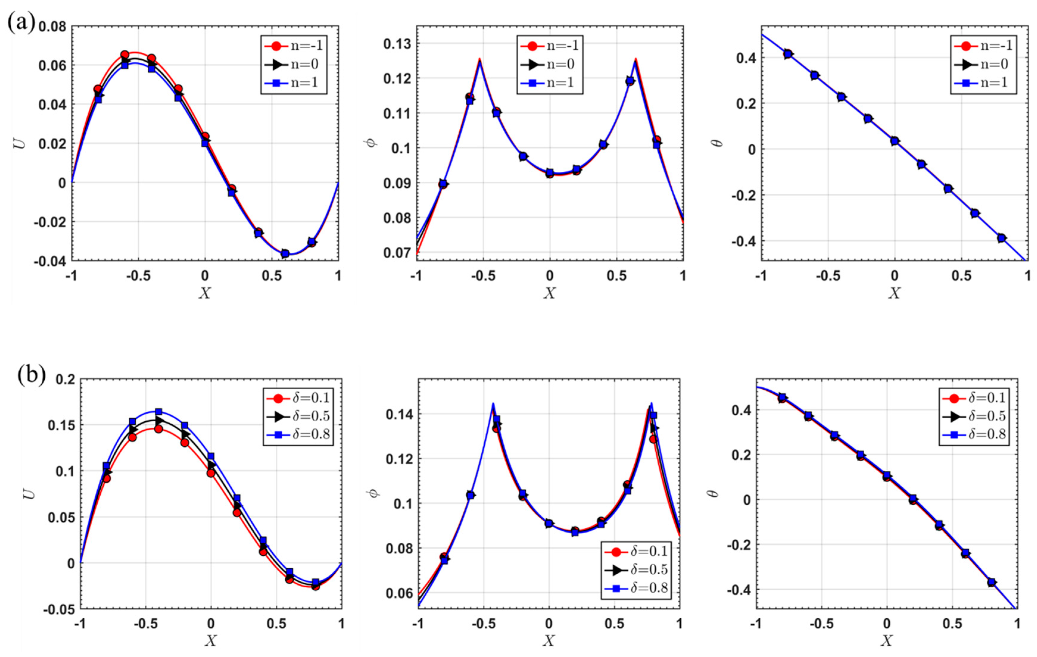
We first perform a parametric study for the case of natural convection of a suspension composed of neutrally buoyant particles in a fluid in a vertical channel; in this case, and . Notice that according to Equation (12) the small size particles can lead to a negligible . Figure 2 shows the effect of the buoyancy force term, . We can observe two approximately parabolic velocity profiles where near the hotter wall the velocity is positive and near the colder wall the velocity is negative; the particles tend to concentrate near the region with the maximum and minimum velocity (low shear rates) due to the effect of the particle flux term ; the temperature shows higher values in the interior of the flow due to the effect of viscous dissipation. As the buoyancy force () increases, the magnitude of the velocity seems to increase, resulting in an increase in temperature. We also notice that more particles accumulate near the region with the maximum and minimum velocity, perhaps due to the higher values of the shear rate, see Equation (12). Figure 3 shows the effect of the shear-dependent viscosity. From Figure 3a, we can see that as the fluid changes from shear-thinning to shear-thickening (n changing from −1 to 1), the magnitude of the velocity tends to decrease; and the temperature and volume fraction profiles change a little for the range of parameters studied here. From Figure 3b, we notice that as increases, implying that the shear-thinning effect is stronger (notice n = −0.5), the magnitude of the velocity increases, while the concentration and temperature profiles do not change that much.
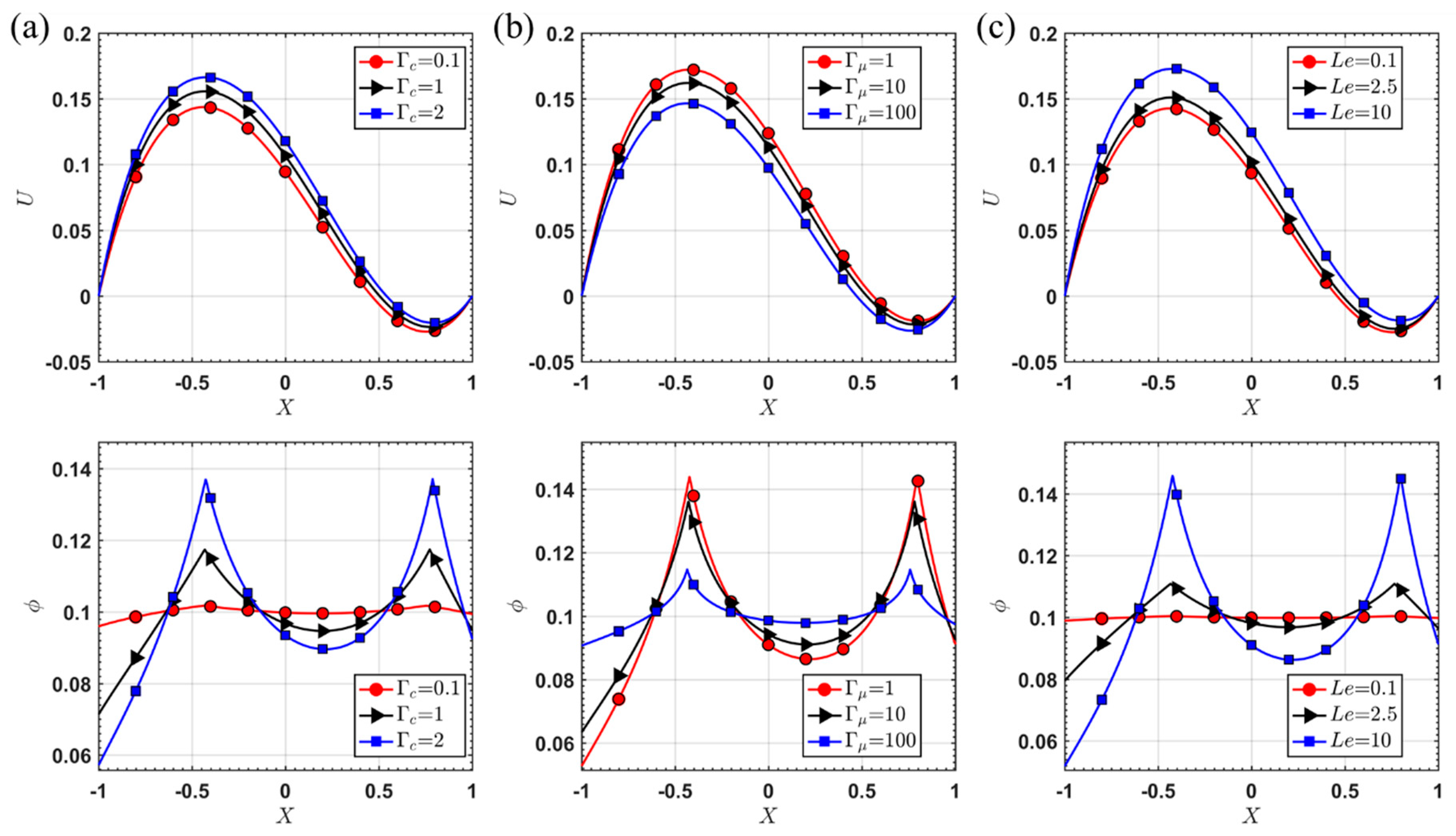
In Figure 4, we can see the effects of particle flux terms, and , and the dimensionless number, . Recall that represents the particle flux responsible for variable shear rates. As Figure 4a indicates, increasing causes the particles to move towards the region with low shear rate, and a small value of (0.1) leads to a uniform distribution of the particles; the velocity seems to increase as increases, since the particle concentration near the region with low shear rate seems to produce a “lubrication” region near the wall. Figure 4b indicates that the effect of is opposite to that of , implying that for the type of suspension considered here, tends to make the particles to be distributed more uniformly. Notice that the viscosity is proportional to the particle concentration, while according to Equation (12) forces the particle to move towards the region with lower viscosity. is proportional to the coefficient of the flux due to the Brownian effects, therefore from Figure 4c, we see that a small value of leads to a uniform distribution of the particles; overall the effect of is similar but opposite to the effect of .
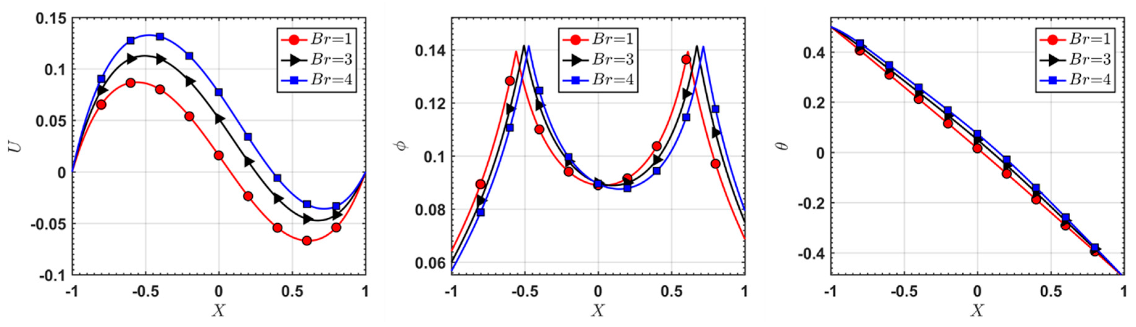
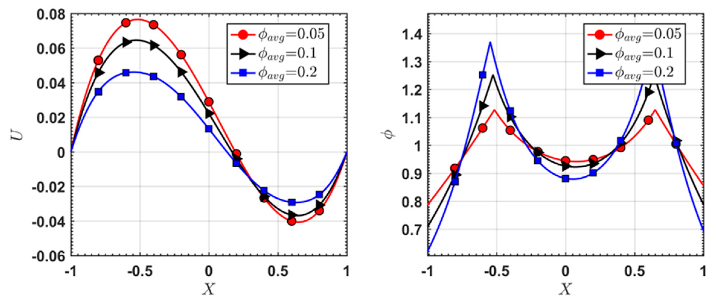
Figure 5 shows the effect of the Brinkman number (). A larger value of indicates an increase in the temperature in the interior region; as a result, the velocity seems to increase indicating an increase in the buoyancy force. The effect of on the concentration profile is moderate, but we see that the position of the maximum concentration moves slightly. Figure 6 shows that as the bulk (average) concentration of the particles, , increases, the magnitude of the velocity decreases, perhaps due to an increase in the viscosity; for particle concentration, a smaller leads to a more uniform distribution of the particles.
5.2. Natural Convection with Particle Sedimentation
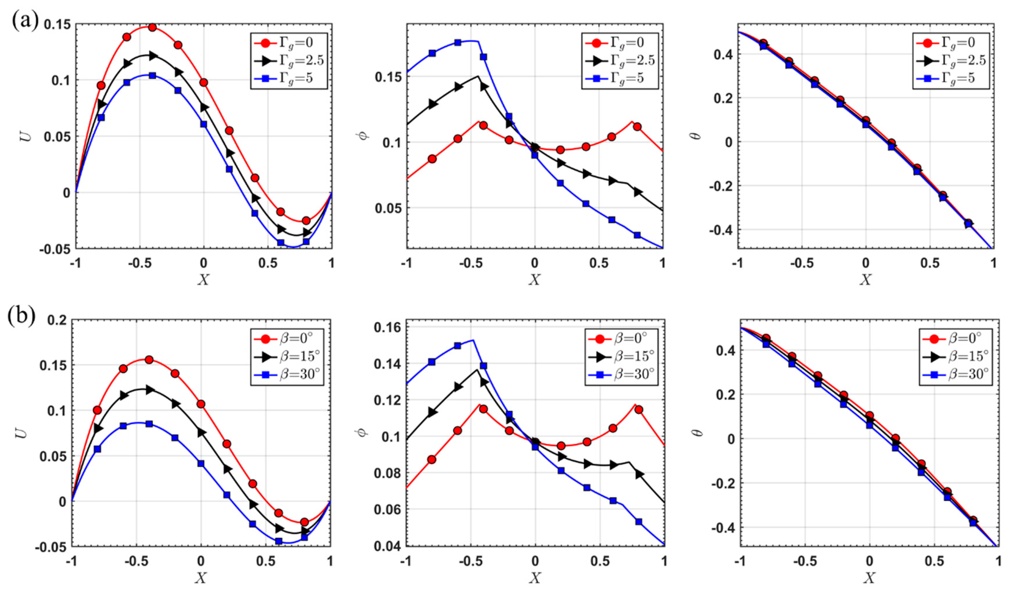
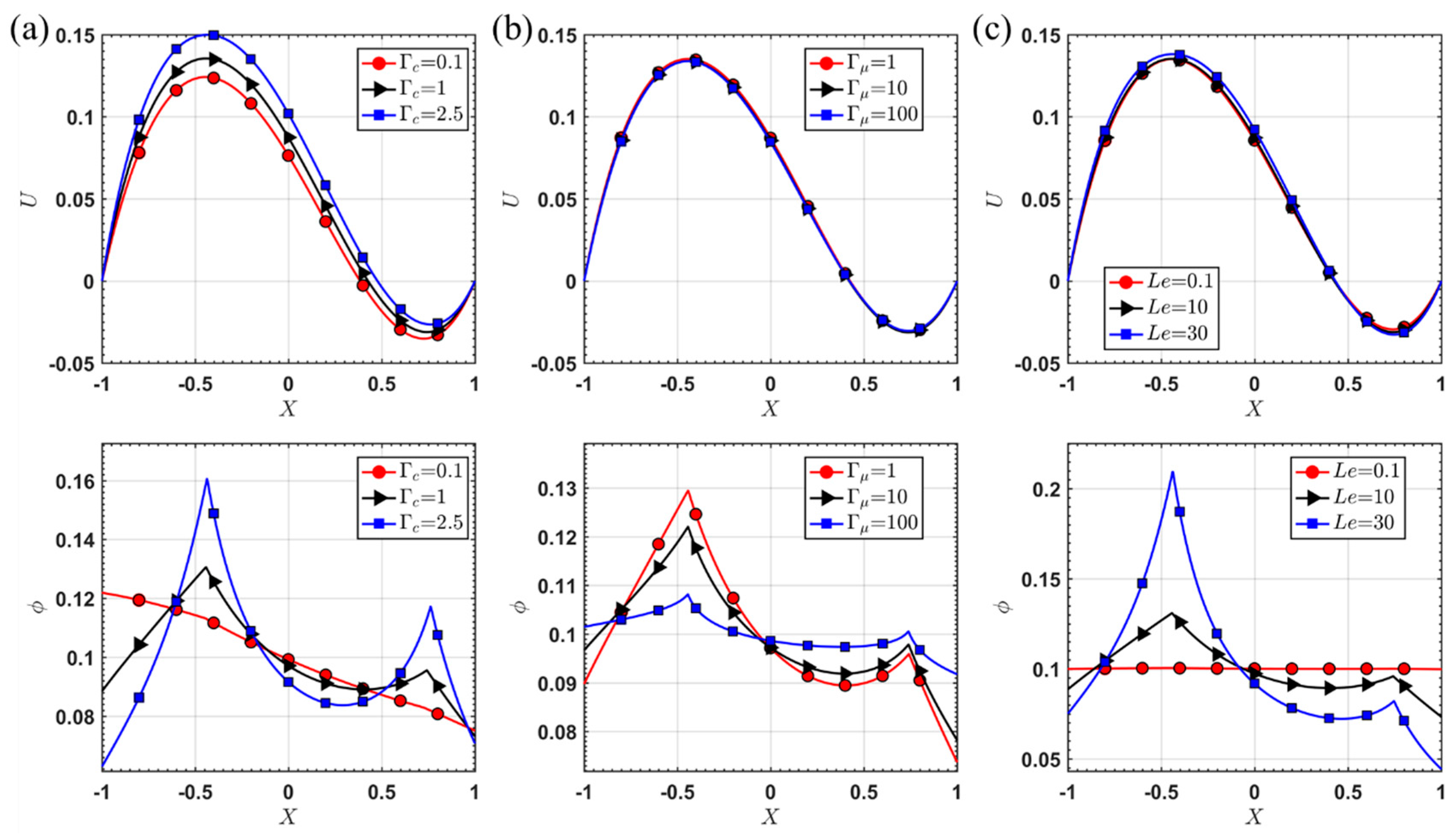
Now we look at a more general situation by considering two parallel walls which are tilted at an angle, giving rise to the possibility that particles may deposit. Figure 7 shows the effect of the particle flux due to gravity. Figure 7a indicates that as increases, more particles tend to move and concentrate near the left wall (X = −1, see Figure 1); the particle concentration near the right wall decreases faster as increases, and when there are almost no particles at the right wall. For the velocity profile, the position of the maximum velocity tends to move slightly toward the left wall, perhaps due to an increase in the particle concentration in that region. Figure 7b shows that as increases, indicating an increase or decrease in the X and Y component of the gravity, the velocity decreases and the particles tend to concentrate near the left wall; the temperatures seem to decrease a little.
Figure 8 shows the effect of . Unlike the case with the neutrally buoyant particles, when has a small value (0.1), the concentration now seems to decrease almost linearly in the X-direction. As increases, the pattern of high particle concentration near the region with larger magnitude of velocity re-appears. Similar to the previous section, the effect of is opposite to that of , as shown in Figure 8b. From Figure 8c, we can see that when is small, that is when the Brownian motion is strong, the particles are more uniformly distributed.
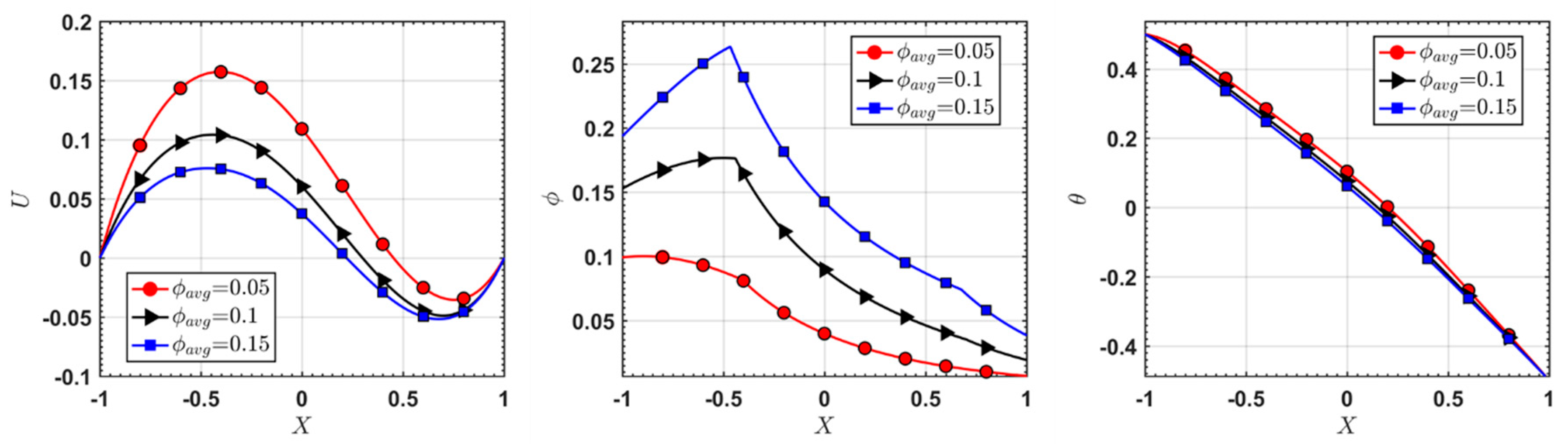
Figure 9 indicates that as decreases, that is as the effect of the buoyancy force becomes less noticeable, particle sedimentation under gravity becomes more significant; meanwhile the values of the velocity and the temperature decrease. It should be noticed that the parametric studies of the Brinkman number (), and the terms related to the shear-dependent viscosity ( and ) are not shown in this section, because the effects are similar to the Section 5.1. Figure 10 shows the effect of the bulk (average) concentration (). With a small value of (0.05), the concentration profile decreases monotonically along the X-direction, indicating that the particle distribution is dominated by the flux term due to gravity. We can also notice that increasing results in a higher viscosity, causing a decrease in the velocity, viscous dissipation and the temperature.
6. Conclusions
In this paper we study the buoyancy driven flow of a suspension between two long vertically inclined walls. The suspension is modeled as a non-linear fluid, where the viscosity depends on the shear rate and the particle concentration. The motion of the particles is modeled by a convection-diffusion equation, where the particle transport flux is assumed to depend on the body force (gravity), and the variation of the shear rate and viscosity. The numerical results indicate that natural convection flow shows certain multi-component features noticed in flow of solid-fluid suspensions where the solid particles tend to move and concentrate near the region with low shear rate. Furthermore, under the effect of gravity, the particles tend to move and concentrate near the lower (left) wall; however, a small Lewis number (stronger Brownian diffusion) can generate a more uniform concentration distribution.
Author Contributions
C.T. and W.-T.W. did the numerical simulations. W.-T.W. and M.M. derived all the equations. M.M. supervised this work. All of the authors have provided substantial contributions to the manuscript preparation.
Funding
This research received no external funding.
Conflicts of Interest
The authors declare no conflict of interest.
Nomenclature
| Symbol | Explanation |
| Density | |
| Specific internal energy | |
| Radiant heating | |
| Specific entropy density | |
| Gravity | |
| Characteristic length | |
| Thermal conductivity | |
| Coefficient of thermal expansion | |
| Shear rate | |
| Coefficients of particle flux | |
| Particle response time | |
| Power-law index | |
| Particle radius | |
| Diffusion coefficient | |
| Viscosity | |
| Temperature | |
| Volume fraction | |
| Pressure | |
| Inclination angle | |
| Spatial position | |
| Velocity | |
| Body force vector | |
| Heat flux vector | |
| Particle flux | |
| Cauchy stress tensor | |
| Gradient of the velocity vector | |
| Symmetric part of the velocity gradient | |
| Identity tensor | |
| Gradient symbol | |
| Divergence operator | |
| Trace operator |
References
- Turner, J.S. Buoyancy Effects in Fluids; Cambridge University Press: Cambridge, UK, 1979. [Google Scholar]
- Chen, B.; Mikami, F.; Nishikawa, N. Experimental studies on transient features of natural convection in particles suspensions. Int. J. Heat Mass Transf. 2005, 48, 2933–2942. [Google Scholar] [CrossRef]
- Sun, X.; Massoudi, M.; Aubry, N.; Chen, Z.; Wu, W.-T. Natural convection and anisotropic heat transfer in a ferro-nanofluid under magnetic field. Int. J. Heat Mass Transf. 2019, 133, 581–595. [Google Scholar] [CrossRef]
- Kang, C.; Okada, M.; Hattori, A.; Oyama, K. Natural convection of water–fine particle suspension in a rectangular vessel heated and cooled from opposing vertical walls. Int. J. Heat Mass Transf. 2001, 44, 2973–2982. [Google Scholar] [CrossRef]
- Bustos, M.C.; Paiva, F.; Wendland, W. Control of continuous sedimentation of ideal suspensions as an initial and boundary value problem. Math. Methods Appl. Sci. 1990, 12, 533–548. [Google Scholar] [CrossRef]
- Metivier, C.; Li, C.; Magnin, A. Origin of the onset of Rayleigh-Bénard convection in a concentrated suspension of microgels with a yield stress behavior. Phys. Fluids 2017, 29, 104102. [Google Scholar] [CrossRef]
- Okada, M.; Suzuki, T. Natural convection of water-fine particle suspension in a rectangular cell. Int. J. Heat Mass Transf. 1997, 40, 3201–3208. [Google Scholar] [CrossRef]
- Batchelor, G.K. Heat convection and buoyancy effects in fluids. Q. J. R. Meteorol. Soc. 1954, 80, 339–358. [Google Scholar] [CrossRef]
- Shenoy, A.V.; Mashelkar, R.A. Thermal convection in non-Newtonian fluids. In Advances in Heat Transfer; Elsevier: Amsterdam, The Netherlands, 1982; Volume 15, pp. 143–225. [Google Scholar]
- Rajagopal, K.R.; Na, T.-Y. Natural convection flow of a non-Newtonian fluid between two vertical flat plates. Acta Mech. 1985, 54, 239–246. [Google Scholar] [CrossRef] [Green Version]
- Massoudi, M.; Christie, I. Natural convection flow of a non-Newtonian fluid between two concentric vertical cylinders. Acta Mech. 1990, 82, 11–19. [Google Scholar] [CrossRef]
- Massoudi, M.; Vaidya, A.; Wulandana, R. Natural convection flow of a generalized second grade fluid between two vertical walls. Nonlinear Anal. Real World Appl. 2008, 9, 80–93. [Google Scholar] [CrossRef]
- Rajagopal, K.R.; Tao, L. Mechanics of Mixtures, Series on Advances in Mathematics for Applied Sciences; World Scientific: Singapore, 1995; Volume 35. [Google Scholar]
- Massoudi, M. Constitutive relations for the interaction force in multicomponent particulate flows. Int. J. Non. Linear. Mech. 2003, 38, 313–336. [Google Scholar] [CrossRef]
- Massoudi, M. A note on the meaning of mixture viscosity using the classical continuum theories of mixtures. Int. J. Eng. Sci. 2008, 46, 677–689. [Google Scholar] [CrossRef]
- Massoudi, M. A Mixture Theory formulation for hydraulic or pneumatic transport of solid particles. Int. J. Eng. Sci. 2010, 48, 1440–1461. [Google Scholar] [CrossRef]
- Slattery, J.C. Advanced Transport Phenomena; Cambridge University Press: Cambridge, UK, 1999. [Google Scholar]
- Liu, I.-S. Continuum Mechanics; Springer Science & Business Media: Berlin, Germany, 2002. [Google Scholar]
- Dunn, J.E.; Fosdick, R.L. Thermodynamics, stability, and boundedness of fluids of complexity 2 and fluids of second grade. Arch. Ration. Mech. Anal. 1974, 56, 191–252. [Google Scholar] [CrossRef]
- Probstein, R.F. Physicochemical Hydrodynamics: An Introduction; John Wiley & Sons: Hoboken, NJ, USA, 2005. [Google Scholar]
- Macosko, C. Rheology: Principles, Measurements and Applications; Wiley-VCH Inc.: New York, NY, USA, 1994. [Google Scholar]
- Schowalter, W.R. Mechanics of Non-Newtonian Fluids; Pergamon Press: Oxford, UK, 1978. [Google Scholar]
- Bridges, C.; Rajagopal, K.R. Pulsatile Flow of a Chemically-Reacting Nonlinear Fluid. Comput. Math. Appl. 2006, 52, 1131–1144. [Google Scholar] [CrossRef] [Green Version]
- Krieger, I.M. Rheology of monodisperse latices. Adv. Colloid Interface Sci. 1972, 3, 111–136. [Google Scholar] [CrossRef]
- Phillips, R.J.; Armstrong, R.C.; Brown, R.A.; Graham, A.L.; Abbott, J.R. A constitutive equation for concentrated suspensions that accounts for shear-induced particle migration. Phys. Fluids A Fluid Dyn. 1992, 4, 30–40. [Google Scholar] [CrossRef]
- Tao, C.; Kutchko, B.G.; Rosenbaum, E.; Wu, W.-T.; Massoudi, M.; Tao, C.; Kutchko, B.G.; Rosenbaum, E.; Wu, W.-T.; Massoudi, M. Steady Flow of a Cement Slurry. Energies 2019, 12, 2604. [Google Scholar] [CrossRef]
- Miao, L.; Massoudi, M. Effects of shear dependent viscosity and variable thermal conductivity on the flow and heat transfer in a slurry. Energies 2015, 8, 11546–11574. [Google Scholar] [CrossRef]
- Yang, H.; Aubry, N.; Massoudi, M. Heat transfer in granular materials: Effects of nonlinear heat conduction and viscous dissipation. Math. Methods Appl. Sci. 2013, 36, 1947–1964. [Google Scholar] [CrossRef]
- Yang, H.; Massoudi, M. Conduction and convection heat transfer in a dense granular suspension. Appl. Math. Comput. 2018, 332, 351–362. [Google Scholar] [CrossRef]
- Massoudi, M. On the heat flux vector for flowing granular materials—Part I: Effective thermal conductivity and background. Math. Methods Appl. Sci. 2006, 29, 1585–1598. [Google Scholar] [CrossRef]
- Massoudi, M. On the heat flux vector for flowing granular materials—part II: Derivation and special cases. Math. Methods Appl. Sci. 2006, 29, 1599–1613. [Google Scholar] [CrossRef]
- Massoudi, M.; Kirwan, A. On Thermomechanics of a Nonlinear Heat Conducting Suspension. Fluids 2016, 1, 19. [Google Scholar] [CrossRef]
- Rajagopal, K.R.; Ruzicka, M.; Srinivasa, A.R. On the Oberbeck-Boussinesq approximation. Math. Model. Methods Appl. Sci. 1996, 6, 1157–1167. [Google Scholar] [CrossRef]
- Rajagopal, K.R.; Saccomandi, G.; Vergori, L. On the Oberbeck–Boussinesq approximation for fluids with pressure dependent viscosities. Nonlinear Anal. Real World Appl. 2009, 10, 1139–1150. [Google Scholar] [CrossRef]
- Subia, S.R.; Ingber, M.S.; Mondy, L.A.; Altobelli, S.A.; Graham, A.L. Modelling of concentrated suspensions using a continuum constitutive equation. J. Fluid Mech. 1998, 373, 193–219. [Google Scholar] [CrossRef]
- Acrivos, A.; Mauri, R.; Fan, X. Shear-induced resuspension in a Couette device. Int. J. Multiph. flow 1993, 19, 797–802. [Google Scholar] [CrossRef]
- Wu, W.T.; Aubry, N.; Antaki, J.F.; Massoudi, M. A non-linear fluid suspension model for blood flow. Int. J. Non. Linear Mech. 2019, 109, 32–39. [Google Scholar] [CrossRef]
- Massoudi, M.; Uguz, A.K. Chemically-reacting fluids with variable transport properties. Appl. Math. Comput. 2012, 219, 1761–1775. [Google Scholar] [CrossRef]
- Bird, R.B.; Stewart, W.E.; Lightfoot, E.N. Transport Phenomena; John Wiley & Sons: Hoboken, NJ, USA, 2007. [Google Scholar]
- Dawson, P.R.; McTigue, D.F. A numerical model for natural convection in fluid-saturated creeping porous media. Numer. Heat Transf. 1985, 8, 45–63. [Google Scholar] [CrossRef]
- Pruša, V.; Rajagopal, K.R. On models for viscoelastic materials that are mechanically incompressible and thermally compressible or expansible and their Oberbeck–Boussinesq type approximations. Math. Model. Methods Appl. Sci. 2013, 23, 1761–1794. [Google Scholar] [CrossRef]
- Massoudi, M. Boundary conditions in mixture theory and in CFD applications of higher order models. Comput. Math. Appl. 2007, 53, 156–167. [Google Scholar] [CrossRef] [Green Version]
- MATLAB User’s Guide; The Mathworks Inc.: Natick, MA, USA, 1998.
Figure 1.
Physical sketch of the system.
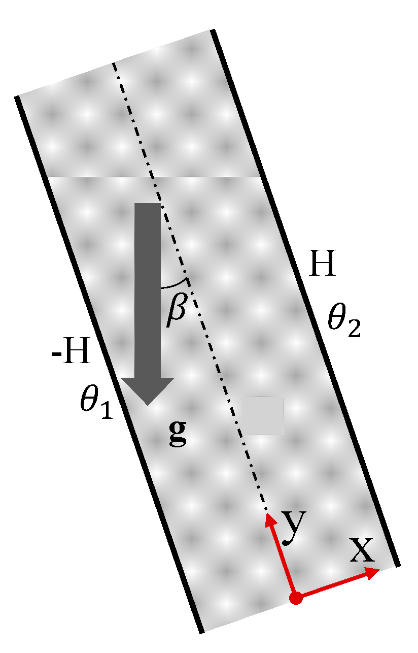
Figure 2.
Effect of the buoyancy force term, the Rayleigh number () on the velocity, concentration and temperature profiles, when , , , , , and .
Figure 2.
Effect of the buoyancy force term, the Rayleigh number () on the velocity, concentration and temperature profiles, when , , , , , and .
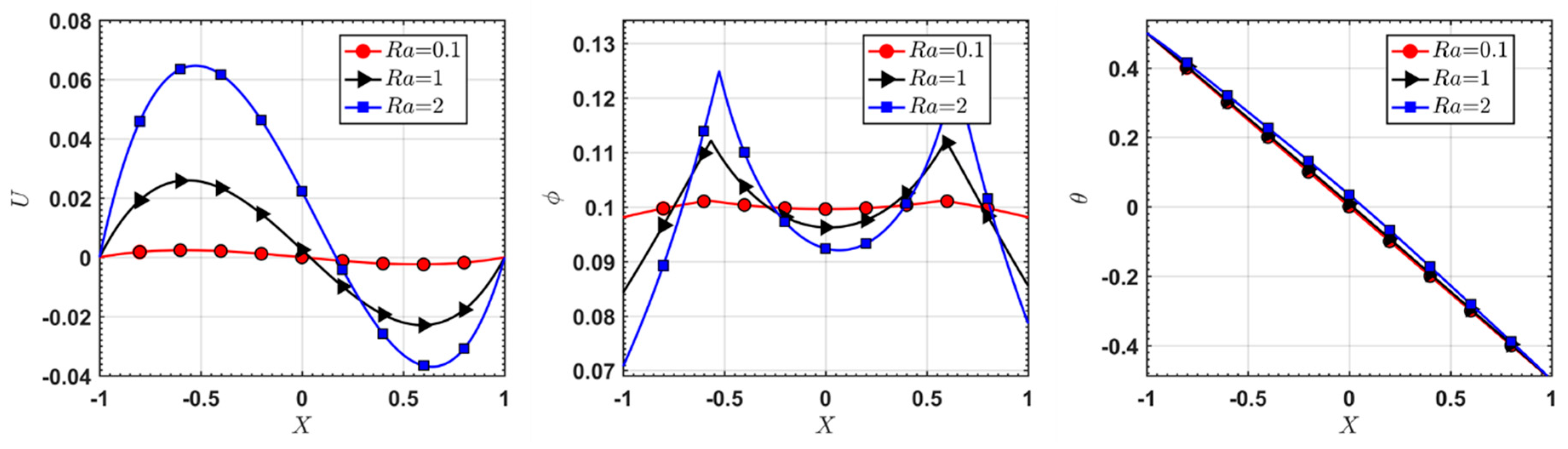
Figure 3.
Parametric studies for shear-dependent viscosity. (a) Effect of on the velocity, concentration and temperature profiles, when , , , , , and . (b) Effect of on the velocity, concentration and temperature profiles, when , , , , , and .
Figure 3.
Parametric studies for shear-dependent viscosity. (a) Effect of on the velocity, concentration and temperature profiles, when , , , , , and . (b) Effect of on the velocity, concentration and temperature profiles, when , , , , , and .

Figure 4.
(a) Effect of on the velocity, and concentration, when , , , , , and . (b) Effect of on the velocity, and concentration, when , , , , , and . (c) Effect of on the velocity, and concentration, when , , , , , and .
Figure 4.
(a) Effect of on the velocity, and concentration, when , , , , , and . (b) Effect of on the velocity, and concentration, when , , , , , and . (c) Effect of on the velocity, and concentration, when , , , , , and .

Figure 5.
Effect of Brinkman number () on the velocity, concentration and temperature profiles, when , , , , , and .
Figure 5.
Effect of Brinkman number () on the velocity, concentration and temperature profiles, when , , , , , and .

Figure 6.
Effect of bulk (average) concentration () on the velocity and concentration profiles, when , , , , , and .
Figure 6.
Effect of bulk (average) concentration () on the velocity and concentration profiles, when , , , , , and .

Figure 7.
Effect of particle flux due to gravity. (a) Effect of on the velocity, concentration and temperature profiles, when , , , , , , , and . (b) Effect of on the velocity, concentration and temperature profiles, when , , , , , , , and .
Figure 7.
Effect of particle flux due to gravity. (a) Effect of on the velocity, concentration and temperature profiles, when , , , , , , , and . (b) Effect of on the velocity, concentration and temperature profiles, when , , , , , , , and .

Figure 8.
Effect of particle fluxes, , and . (a) Effect of on the velocity and concentration profiles, when , , , , , , , and . (b) Effect of on the velocity and concentration profiles, when , , , , , , , and . (c) Effect of on the velocity and concentration profiles, when , , , , , , , and .
Figure 8.
Effect of particle fluxes, , and . (a) Effect of on the velocity and concentration profiles, when , , , , , , , and . (b) Effect of on the velocity and concentration profiles, when , , , , , , , and . (c) Effect of on the velocity and concentration profiles, when , , , , , , , and .

Figure 9.
Effect of buoyancy force term, Rayleigh number () on the velocity, concentration and temperature profiles, when , , , , , , , and .
Figure 9.
Effect of buoyancy force term, Rayleigh number () on the velocity, concentration and temperature profiles, when , , , , , , , and .
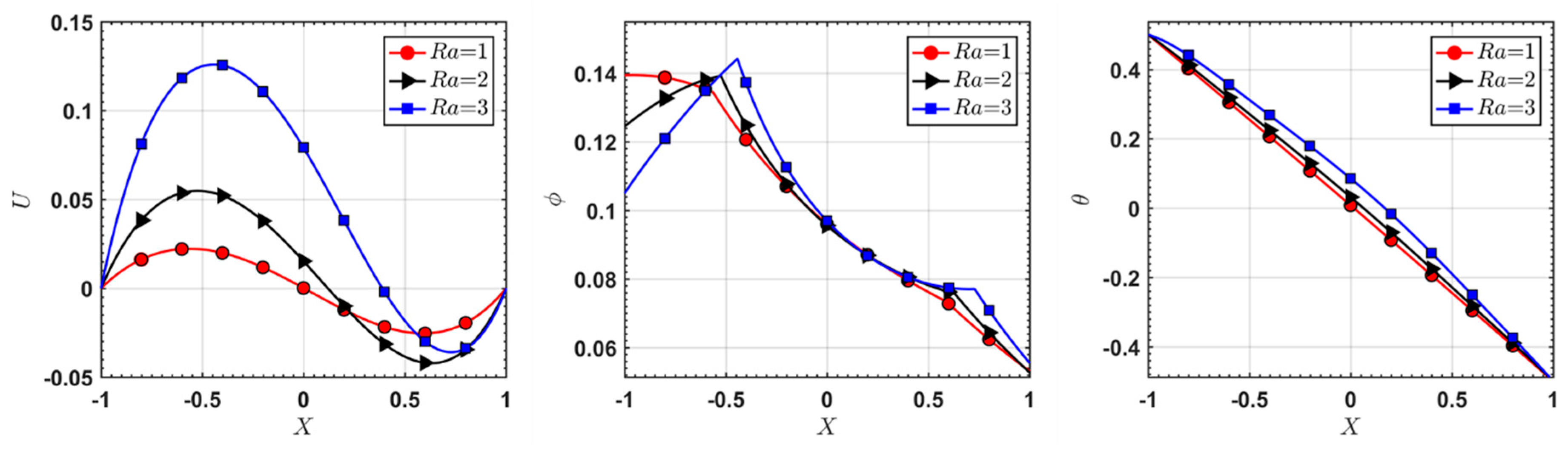
Figure 10.
Effect of bulk (average) concentration () on the velocity, concentration and temperature profiles, when , , , , , , , and .
Figure 10.
Effect of bulk (average) concentration () on the velocity, concentration and temperature profiles, when , , , , , , , and .


Table 1.
The dimensionless parameters used in our study.
| Section 5.1 | Section 5.2 | ||
|---|---|---|---|
| 0.1, 1.0, 2.0 | . | 1.0, 2.0, 3.0 | |
| 0.1, 1.0, 2.0 | 0.1, 1, 2.5 | ||
| 1, 10, 100 | 1, 10, 100 | ||
| 0.1, 2.5, 10 | 0.1, 10, 30 | ||
| 0.5, 0.0, 1 | NA | ||
| 0.1, 0.5, 0.8 | NA | ||
| 1, 3, 4 | NA | ||
| 0.05, 0.1, 0.2 | 0.05, 0.1, 0.15 | ||
| NA | , , | ||
| NA | 0, 2.5, 5 | ||
© 2019 by the authors. Licensee MDPI, Basel, Switzerland. This article is an open access article distributed under the terms and conditions of the Creative Commons Attribution (CC BY) license (http://creativecommons.org/licenses/by/4.0/).
Share and Cite
MDPI and ACS Style
Tao, C.; Wu, W.-T.; Massoudi, M. Natural Convection in a Non-Newtonian Fluid: Effects of Particle Concentration. Fluids 2019, 4, 192. https://doi.org/10.3390/fluids4040192
AMA Style
Tao C, Wu W-T, Massoudi M. Natural Convection in a Non-Newtonian Fluid: Effects of Particle Concentration. Fluids. 2019; 4(4):192. https://doi.org/10.3390/fluids4040192
Chicago/Turabian StyleTao, Chengcheng, Wei-Tao Wu, and Mehrdad Massoudi. 2019. "Natural Convection in a Non-Newtonian Fluid: Effects of Particle Concentration" Fluids 4, no. 4: 192. https://doi.org/10.3390/fluids4040192