Bathymetry Development and Flow Analyses Using Two-Dimensional Numerical Modeling Approach for Lake Victoria

Abstract

This study explored two-dimensional (2D) numerical hydrodynamic model simulations of Lake Victoria. Several methods were developed in Matlab to build the lake topography. Old depth soundings taken in smaller parts of the lake were combined with more recent extensive data to produce a smooth topographical model. The lake free surface numerical model in the COMSOL Multiphysics (CM) software was implemented using bathymetry and vertically integrated 2D shallow water equations. Validated by measurements of mean lake water level, the model predicted very low mean flow speeds and was thus close to being linear and time invariant, allowing long-time simulations with low-pass filtered inflow data. An outflow boundary condition allowed an accurate simulation to achieve the lake’s steady state level. The numerical accuracy of the linear measurement of lake water level was excellent.

1. Introduction

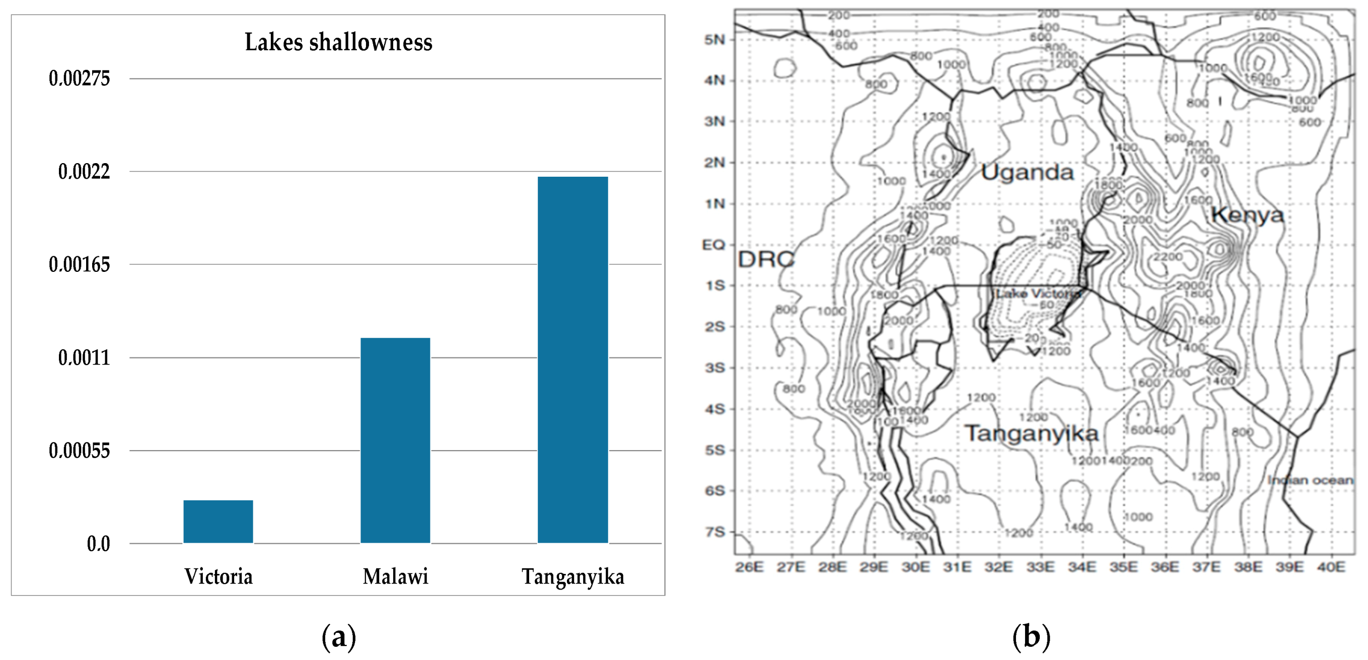
Lake Victoria (LV) in East-Africa is the second largest fresh water body in the world and the largest in Africa, with a shoreline shared by three countries: Uganda, Kenya, and Tanzania. It is a shallow water body with an average depth of 40 meters and a maximum depth of 80 meters, and a horizontal extent of 355 km [1,2]. The largest fresh water body in East-Africa is now severely affected by water quality degradation. The most important components of water quality degradation are: Pollution, river discharge, sedimentation, nutrient loading, and eutrophication. The lake is also greatly affected by many other factors due to its shallowness.

The shallow water body system is environmentally sensitive and its flow management areas are complex [3]. Climate change, or at least the fact that extremes are increasingly appearing, has changed the vulnerability of the flow of shallow water bodies. There is a need to understand the hydrodynamic processes of lake systems that are directly affected by chemical, biological and ecological systems as well as the physical processes of the lake system and their driving forces, which are crucial for the management of these systems [4]. Previous Lake Victoria model analyses [5,6,7,8], including thermodynamic and hydrodynamic characteristics, were based on the Princeton Ocean Model 3D simulations. They considered an elliptic lake with surface wind stress to investigate the vertical lake temperature profiles. Nyamweya et al. [9] used the Regional Oceanographic Model System (ROMS) to investigate Lake Victoria’s physical processes (temperature and currents) that have an effect on dial, seasonal, and annual variations in stratification, vertical mixing and inshore-offshore exchanges. They developed the model in ROMS to better understand annual and seasonal water circulation in Lake Victoria based on real bathymetry, wind stress, surface heat fluxes, solar radiation, and river inflow/outflow forcing. National Oceanic and Atmospheric Administration (NOAA) also built a model for Lake Victoria using meteorological data, with a strategic plan to build an integrated physical and ecological model focusing on eutrophication by 2022 [10]. Analysis of Lake Victoria’s water level, pollution, eutrophication, and sediment flow have been partly covered by Hecky and Kendall [11,12]. However, there has not as yet been any research to consider lake hydrodynamics using details from Lake Victoria’s bathymetry survey.

The Lake Victoria Environment Management Project (LVEMP) reports [12] for the Lake Victoria Basin Commission (LVBC) present a regional water quality synthesis for Lake Victoria, which recommends undertaking a detailed bathymetric survey for Lake Victoria to support model development, calibrations, validation, and investigation of lake residence time. The existing hydrographic chart is out-dated and cannot be used for inshore areas where significant local changes have occurred, due to sedimentation and the river delta extension. The current paper partly follows this recommendation.

In November 2014, the present bathymetry model was presented in [13], which is available on the COMSOL website [13]. The study included different systematic methods for the development of a detailed bathymetry model for a lake hydrodynamic. The Hamilton group created a high-resolution bathymetric Geographic Information System (GIS) raster map, which was made available in October 2016 [14] and further improved in 2018. The data points came from Admiral maps and field data, and were modified for shoreline, consistency etc. [15].

An efficient approach to support and complement the understanding of physical processes in reservoirs is useful for numerical and hydrodynamic modeling [16,17]. One approach in the application of a numerical model for shallow water bodies is the vertically integrated method. Parker and Lenhard [18] used the vertically integrated method for a water and hydrodynamic model to reduce dimensionality and diminished nonlinearity. Strack and Ausk [19] demonstrated that the gradient of the comprehensive discharge potential gives the vertically integrated discharge value throughout the aquifer.

This study included different methods for lake bathymetry development in Matlab. The governing equations were the vertically integrated Saint–Venant shallow water equations (SWEs), which cover the areas of the bottom topography as well as the free surface of the whole lake. The model needed flow sources and fluxes on lake surface areas and lake flow boundaries and used river discharges–inflows as well as the only outflow, the Nile, along the lake shoreline. The model also needed precipitation as well as evaporation on the lake surface, extrapolated from stations on the lakeshore.

This study posed the following scientific questions:

• How are the systematic methods developed for lake bathymetry relevant for lake numerical and hydrodynamic modeling?
• How are lake bathymetry and flow models developed in CM?

To address these questions, the study was designed to:

• Identify specific challenges in building lake bathymetry and exemplify how to overcome them;
• illustrate the improvement of systematic methods for lake bathymetry using Matlab, and analyze 2D surface flow through the numerical model approach in CM;
• assess the reliability of the vertically integrated model by checking its prediction of mean water level;
• explore the relationship between lake outflow conditions and water levels to achieve a steady-state level and numerical accuracy of linear measurement of the lake’s water level;
• discuss the significance of systematic methods for lake bathymetry and the numerical hydrodynamic insights gained from model development.

2. Study Area and Methodological Approach

2.1. Study Area: Lake Victoria

Lake Victoria is the largest tropical lake in the world. It is located between the Eastern and Western Branches of the East African Rift System and lies within an elevated plateau in the western part of Africa’s Great Rift Valley. It occupies a shallow depression (75 m deep) on the Equatorial Plateau (ALT. 1135 m) between two arms of the Great Rift Valley, and has an irregular shoreline, several small islands, and numerous streams (Figure 1b). Its total catchment area is 251,000 km², of which 68,800 km² is the actual lake surface [20]. Its shoreline is shared by Kenya (6%), Uganda (45%), and Tanzania (49%) [21,22], and the tributary areas are composed of many sub-basins in riparian states of Kenya (21.5%), Uganda (15.9%), Tanzania (44.0%), Rwanda (11.4%), and Burundi (7.2%) [23]. Lake Victoria stretches 412 km from north to south, between latitudes 0°31′N and 3°12′S, and 355 km from west to east between longitudes 31°37′W and 34°53′E (Figure 1b). It has a volume of 2,760 km³ [1] and is much shallower than other large African lakes (Malawi and Tanganyika) (Figure 1a).

2.2. Methodological Approach

Numerical modeling is the best tool available when experimental techniques are time-consuming, difficult, or actually impossible. A numerical lake topographical model can provide better information/processing scenarios for hydrological processes. Lake hydrodynamic processes are highly varied due to the lake geometry and surrounding topography, hydrological and geochemical loading, as well as meteorological exposures [24]. Numerical hydrodynamic lake models have recently been used to address environmental problems as well as hydro-meteorological properties and geographical geometric characteristics [25]. The numerical model is solved by the SWEs and considers the Coriolis effect for lake bottom topography [26,27]. In Lake Victoria, Coriolis effects play less of a role because the lake is situated on the equator.

Two-dimensional depth-averaged models for fresh water bodies are used to simulate irregular geometry, steady and unsteady flows, finite difference and finite volume, and finite element methods are used to solve shallow water models [28]. Finite element spatial discretization is attractive for flexibility of triangulation for the representation of irregular boundaries and local mesh refinement [29].

In this study, CM^® was chosen as a platform, since it allows dissimilar physics to be dealt with numerically within the same modeling framework. This is in constrast with the common approach, which treats problems from different disciplines with numerical models specifically developed for their respective discipline. Matlab^® is a multi-paradigm numerical computing environment and proprietary programming language. Matlab libraries for Kriging [30] and triangulation are used to make a smooth lake topographical model.

CM is useful for its:

• Documented equation-based modeling for all relevant physics. For example this supports validation against other simulation platforms, such that the effects of different numerical techniques can be distinguished;
• easy inclusion of equation-based dispersion, biological and chemical processes supported by the Multiphysics features;
• educational effect of a well-developed link between Multiphysics and Matlab with its eclectic numerical libraries;
• so-called COMSOL Server, where a COMSOL Multiphysics application can be run in major platforms such as Windows, Linux, etc. COMSOL Server is a multiuser service that can be run continuously on the host computer, and COMSOL can be run on multiple computers to support simultaneous users and more concurrent applications than could be supported by a single computer. The COMSOL Server service significantly facilitates cooperation between users distributed over different locations, as is the case in the present study where the participating researchers and collaborators are located in Sweden, Uganda, Tanzania and Kenya.

Numerical Simulation in Other Softwares

The numerical modeling was to mainly be realized by means of COMSOL Multiphysics, and comparative studies possibly carried out with some other state-of-the art software such as Delft3D, MikeSHE, ELCOM, GeoClaw, etc. Delft3D is a well-known comprehensive state-of-the art model that is typically used for coastal waters and estuaries. Therefore, before building the model in COMSOL, a few preliminary tests were carried out using Delf3D in order to become acquainted with this particular software as well as with data input and output.

3. Materials and Methods

The first task was to define the lake’s geometry, i.e., the shoreline and bathymetry. The bathymetry was built from several sources, requiring stitching and smoothing operations. The sources and sinks of water, i.e., inflows and outflows, and, where relevant, the solute, evaporation, and precipitation were defined from existing measurements or assessments. A numerical model needs verification or validation before model predictions are considered credible. If widely used general software is employed, verification is a minor issue. However, validation is a major issue for hydrodynamic models, since the required data on water velocity or accurate water levels must be available. The only validation of the present model was a comparison of mean water levels. This validation is only a test of the conservation properties of the numerical model, albeit one that illustrates that the choice of boundary conditions is important.

3.1. Lake Bathymetry

Lake surface elevation is probably the most fundamentally important property, and lake bathymetry is relevant for a wide range of research topic and societal needs. Knowing the exact water depth or morphology of the lake bottom topography is vital, however, its underwater equivalent remains uncertain in lakes, rivers, and oceans in many parts of the world [31]. This work covers the obtaining and merging of raw data as well as filtering and interpolation into a digital elevation model (DEM) to be imported into the simulation software.

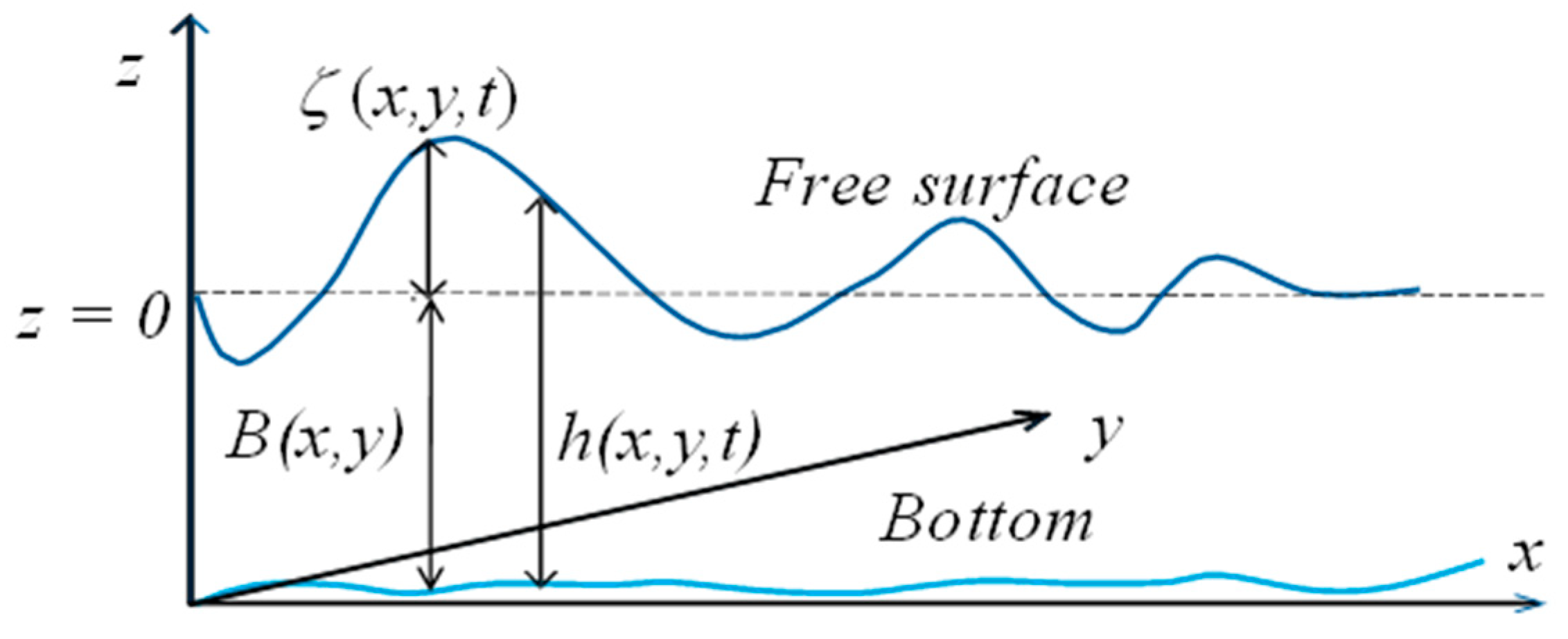
Bathymetry $B\left(x,y\right)$ is a map of the elevation of the “bed” or “floor” of a waterbody. It is assumed that the model has bottom topography fixed in time. The free-surface vertical position from a reference datum, often referred to as wave height, is:

$$z=\zeta \left(x,y,t\right)$$

(1)

Water depth is:

$$h(x,y,t)=B\left(x,y\right)+\zeta \left(x,y,t\right)$$

(2)

where, $z$ is the vertical coordinate, $\zeta$ is the celerity, and $h$ the water depth, as presented in Figure 2. The required data also include the localization of the tributary inflows and the outflow on the shoreline.

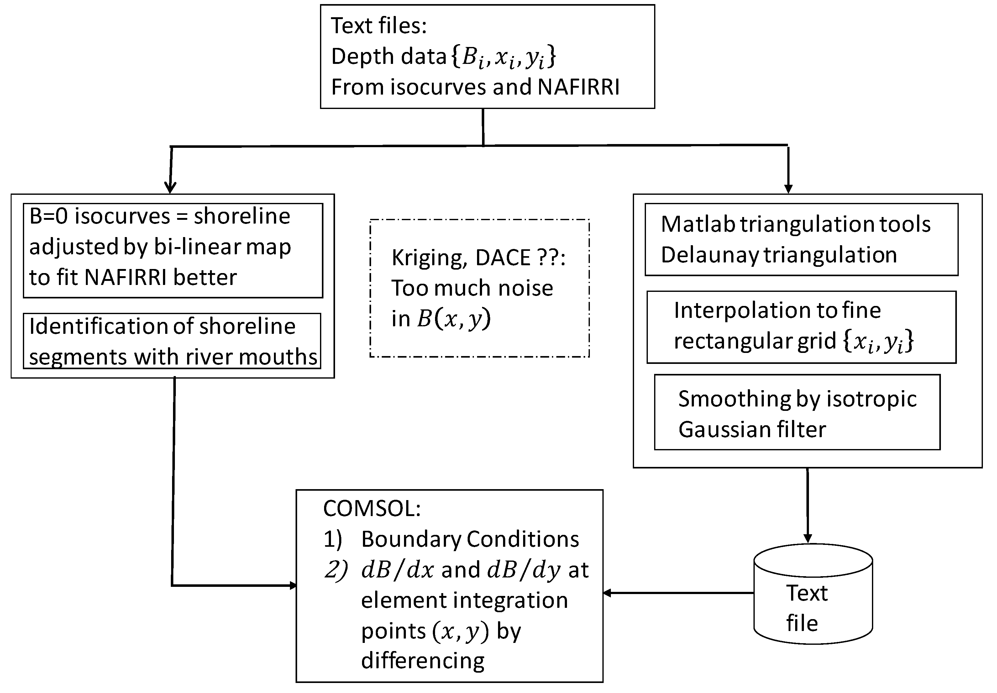
The lake bathymetry was implemented as presented in the flowchart (Figure 3).

3.2. Lake Bathymetry Methods

3.2.1. Digital Elevation Model (DEM) for Lake Bathymetry

An accurate representation of lake topography is essential for lake hydrodynamics. An elevation model contains specific elevation values at specific locations [32]. Conventionally, the values are collected from maps and field surveys. For computer simulations the representation of the topography is called a DEM. Commonly, the model is represented by a rectangular grid, also called an elevation matrix structure, by a triangulated irregular network (TIN) or by contours [33]. NASA (STRM: Shuttle Radar Topography Mission) and U.S. Geological Survey (USGS) are open sources providing geological images, including satellite data, which make data available in different DEM formats. When the work started (2014) [13], no such open source was available for Lake Victoria bathymetry. The model has data from old depth soundings taken in different regions and old depth contours, which were merged with modern echo-sounding data, as presented in [13].

In the autumn of 2017, the HARVARD Dataverse (Hamilton group) made a lake depth map accessible online [14]. The group produced 100 m² GIS-raster maps from SRTM data sources to generate a high-resolution digital elevation model (DEM) of Lake Victoria using raster interferometry. Hamilton group has created a bathymetry model resolution for Lake Victoria. They used old data points (before 20th Century data manually digitized via a process of fitting admiralty maps to the lake shoreline) combined with GPS-enabled (2010) hydrographic survey systems. The raster model was created by the process of simple Kriging. This was unable to capture the deepest portions of Lake Victoria. Continued improvements will follow once more data is captured for Lake Victoria [14].

3.2.2. Coordinates

Let $\theta$ be the latitude, $0$ at the equator and $+90$ on the North Pole. $\phi$ is the longitude, $0$ at Greenwich (UK) and increasing east $(+)$. The lake extent is small enough to be considered a plane normal to gravitational acceleration, $x$ west–east, and $y$ south–north. Thus, as in Equation (3):

$$\left(x,y\right)\approx R\left(\cos {\theta }_0\left(\phi -{\phi }_0\right),\theta -{\theta }_0\right)$$

(3)

where, $R$ is the earth’s radius, $6371\mathrm{km},$ and ${\phi }_0,{\theta }_0=0$ is a central point in the lake.

3.2.3. Depth Data from Several Sources

The available depth data come from two sources:

• An existing Admiral bathymetry map merged with iso-depth curves [34] (Figure 4a);
• modern digitized sets of points obtained from the National Fisheries Resources Research Institute (NaFIRRI), Jinja, Uganda [35] (Figure 4b).

Satellite spectral remote sensing and echo sounders were used. The satellite data covered the lake surface and extended 15 km east–west and south–north of the lake (Figure 4b).

The bottom slopes are the driving forces for the hydrodynamic model that consequently requires $\left(\partial B/\partial x,\partial B/\partial y\right)$ at the integration points of the finite element mesh. This is a scattered data interpolation task, from giving depth data points to finite element integration points. It is accomplished by first creating a $N_x\times N_y$ rectangular grid of $B(x,y)$, dense enough to allow differentiation by differences. Several methods have been used for the unstructured interpolation problem. Since derivatives are needed, the task is challenging.

Two methods were applied in an attempt to create the table $B(X_i,Y_j)$: A Kriging method, as implemented in the MATLAB DACE toolbox (Section 3.2.4), and a Delaunay triangulation of the points followed by interpolation and spatial filtering by an isotropic Gaussian kernel (Section 3.2.5).

The old data with a well-defined shoreline B(x, y) = 0 also had to be combined with the much more voluminous modern data. There were obvious discrepancies in the locations. The fusion of the data is described in Section 3.2.6 below.

3.2.4. Interpolation by Kriging and DACE

Kriging is a geostatistical interpolation technique that is widely used in the design and analysis of computer experiments for response surface models, meta models, and surrogate models. DACE (design and analysis of computer experiments) is a MATLAB toolbox for implementation of a Kriging approximation [30]. The DACE toolbox uses two important functions: Dacefit and predictor. The lake bathymetry development used the DACE toolbox with Delaunay under dacefit functions that created a Kriging interpolation function to determine depth from all the available set of points. This combination process either made interpolation very unsmooth or too smooth to evaluate the $N_x\times N_y$ dense rentangular grid. The main reasons for this are that the initial set of points are anisotropic, the distance between points on cueves is relatively short, and the distance between curves is rather long.

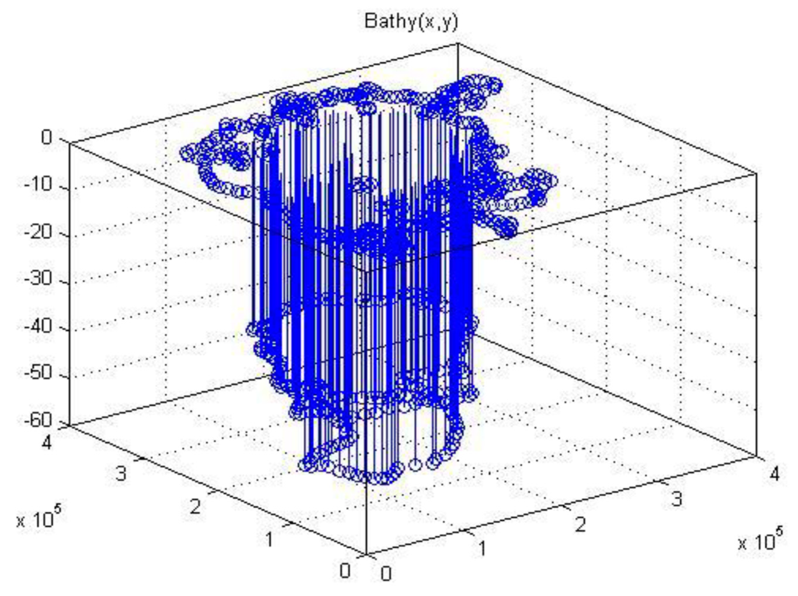
Gridded data in Matlab means the order of data in a grid. A grid is not only a set of points within a certain geometry property; it relies on an ordered relationship between points in the grid, and this structure is very useful for grid-based interpolation. Matlab provides different functions such as Cartesian axis-aligned or array space-aligned for built-in 2D (Figure 4a) and 3D (Figure 5) grid-based interpolation. At this point, is should be noted that $\frac{db}{dx}, \frac{db}{dy}$ was needed to import 2D gridded data in CM.

Kriging considers the data as samples of a stochastic field for which the best linear unbiased estimator is to be obtained. It relies on the variogram $R(x,y)$, which describes how the covariance of the data at two points depends on the relative location of the points. In the estimate, at point $(x,y)$, the influence of data points $\left(x_i,y_i\right)$ decays like the variogram. DACE supports variograms of the form Equation (4),

$$\Re \left(x,y;x_i,y_i\right)=\Re (d),d=\sqrt{{\left(\left(x-x_i\right)/R_x\right)}^2+{\left(\left(y-y_i\right)/R_y\right)}^2}$$

(4)

where, $R_x$ and $R_y$ represent the correlation lengths. These must be chosen to create the estimator, and the automatic procedure implemented in DACE is a nonlinear minimization. This approach becomes more difficult when the data distribution is very different from being essentially isotropic. In the present case, the points are on a few densely sampled curves so the distances between points on the curves are much shorter than the distances between the curves. Extensive manual trial-and-error choices of $R_x$ and $R_y$ were also unable to produce smooth, accurate interpolants for lake topography.

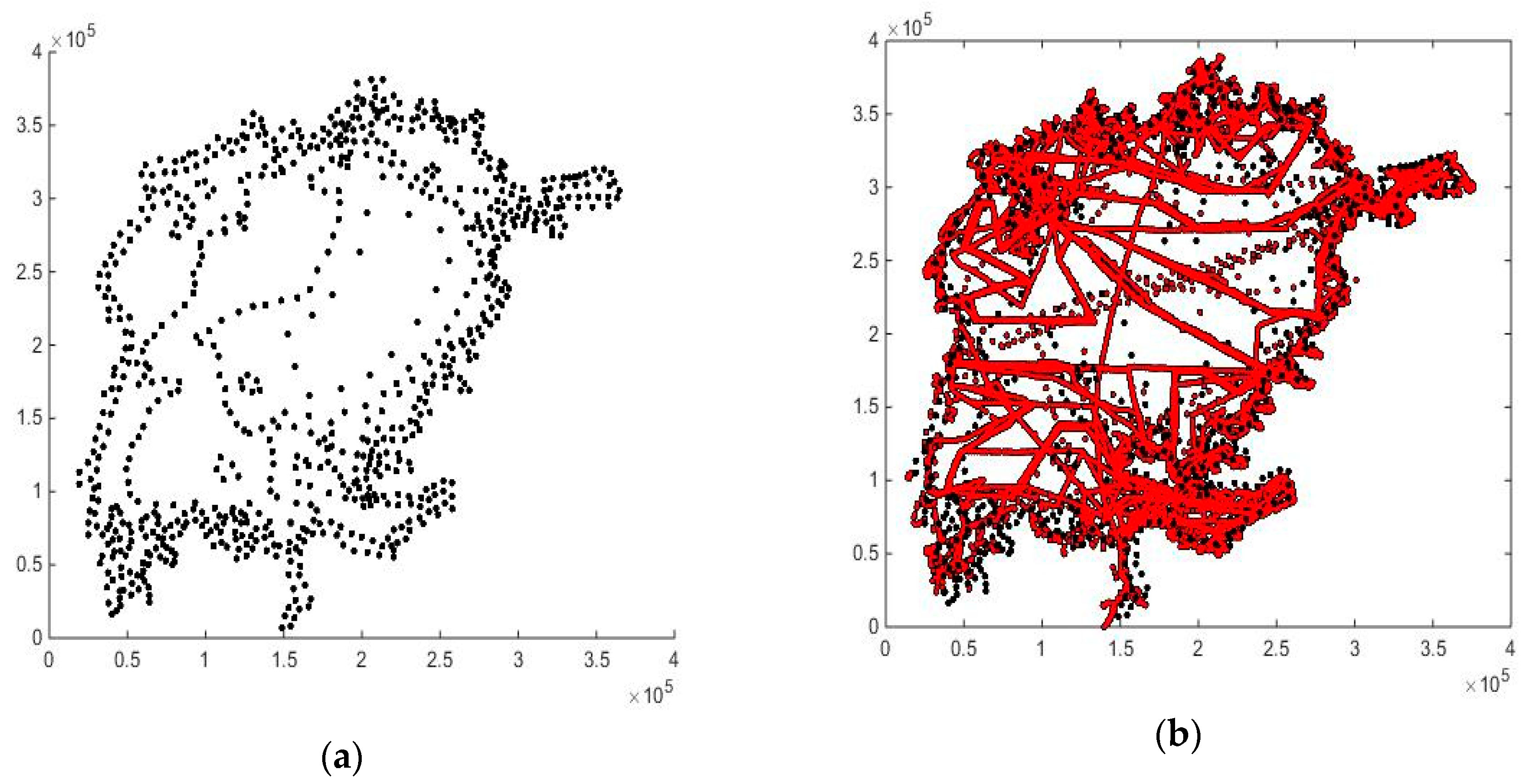
3.2.5. Delaunay Triangulation and Interpolation

The Delaunay triangulation is an essentially uniquely defined, minimum edge length triangulation [36] of the convex hull of a given point set. The circumcircle of each triangle contains only the points that are vertices of that triangle. It is widely used for finite element mesh generation and for scattered data interpolation, and can be computed in O (n log n) time for n points.

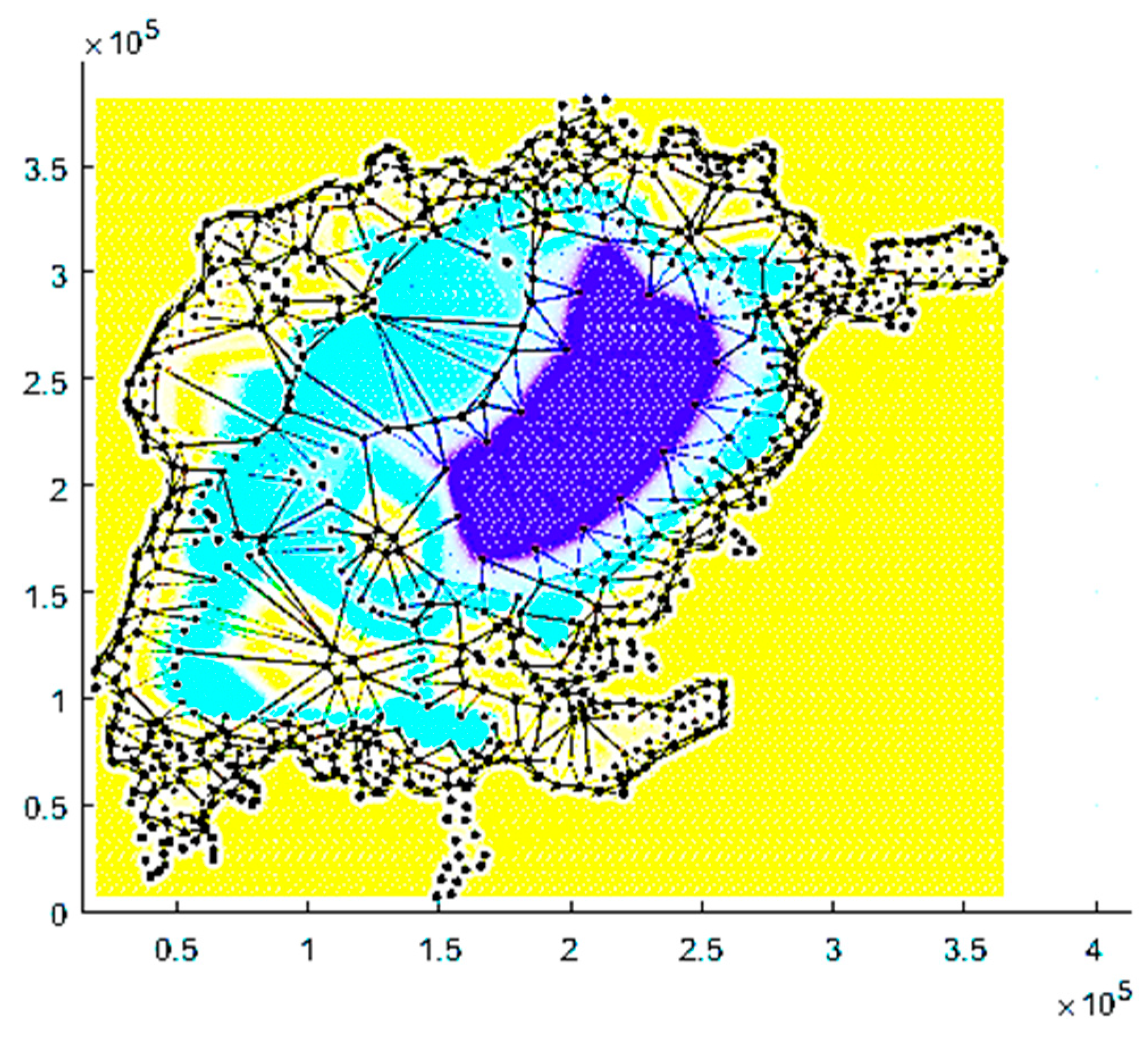
The Delaunay structure was used to interpolate a fine $N_x\times N_y$ rectangular grid covering the convex hull of the set of points. The Matlab function grid data accomplishes these two steps. It was observed that some triangles in the shore regions had all the vertices on the shoreline and thus vanishing depth. Near-shore points were then added manually to avoid such configurations. Figure 6 illustrates the Delaunay triangulation of the old iso-curve data plus the added points. Some of the data points are shadowed in the plot by depth coloring.

The Delaunay interpolant is only continuous (see Figure 6), however, the model requires slopes, i.e., a smooth interpolant. Thus, the grid data were subsequently filtered by an isotropic Gaussian filter with a width chosen as a compromise between the relationship to the data and smoothness.

3.2.6. Merging Iso-Curve Data with NaFIRRI Data

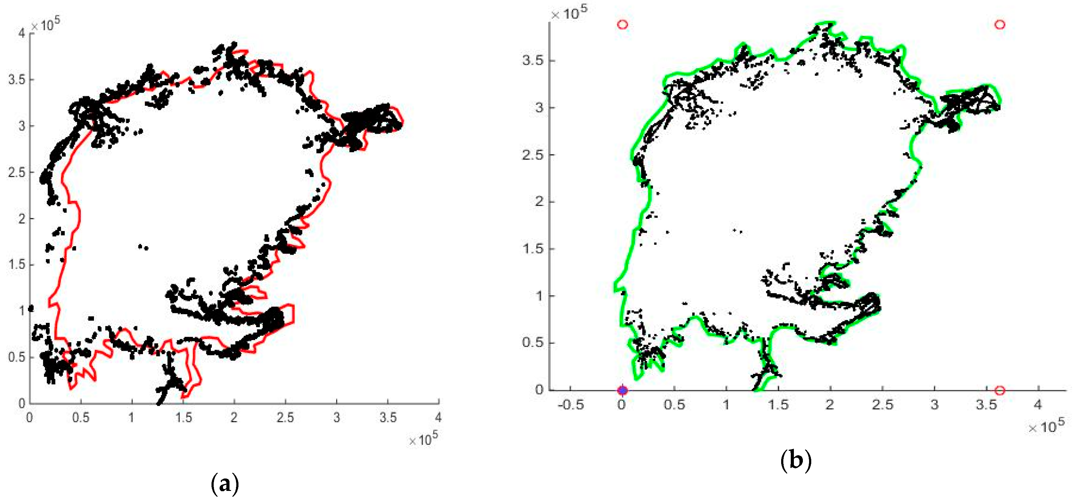
The shore geometry was well defined as a zero depth level curve in the old data points. The NaFIRRI data points did not explicitly show the shoreline. When the older iso-depth curve data points (Figure 4a) were added to the set of NaFIRRI points in a 0–10 m depth, there was an obvious discrepancy in the shoreline (Figure 7a). In order to avoid these problems, the locations of the new data points were slightly modified by a bilinear free-form deformation [37] transformation, defined by 2 × 2 control points at the corners of a rectangle covering the convex hull of the points. This procedure is a fitting of one point cloud C1 ordered along a curve—the shoreline—to another, unordered set C2, easily accomplished by interactive manipulation of the control points. More “objective” algorithms, such as the iterative closest-point scheme [38], try to minimize the mean square distance between C1 and its closest neighbors in C2, and often rely on human help to choose candidate close neighbors (Figure 7b).

4. Governing Equations, Boundary Conditions and Mesh Geometry

4.1. Saint–Venant Shallow Water Equations

Shallow water equations (SWE) are based on the assumption H/L << 1 where H and L are the characteristic values for vertical (i.e., depth) and horizontal length scales, respectively [39,40]. SWE are normally used for large-scale surface areas [26] to simulate tidal flow, surface runoff, coastal flows, dam-break floods, and tsunamis, etc. SWE describes motions in a thin layer of fluid of constant density in hydrostatic balance, bounded from below by the bottom topography and from above by a free surface, in response to gravitational and rotational accelerations [41,42] in addition to inflow/outflow and other sources.

SWE are a system of hyperbolic partial differential equations (PDE). A formulation in terms of the conserved quantities (mass and momentum) is needed if shocks (hydraulic jumps) might appear [43]. Any stable numerical scheme for solving hyperbolic equations must include dissipation. This can be included in the scheme (and hidden from the user), such as in upstream or discontinuous Galerkin schemes, or added as artificial dissipation/diffusion/viscosity terms which are tunable by the user [43]. CM uses the standard Galerkin formulation with artificial dissipation. This makes the equations parabolic, which implies that one boundary condition per-equation is needed for well-posedness. Such stabilization is added automatically for CM Computational fluid dynamics (CFD) modules, however, the SWE must be modelled by equations and the dissipation must be added explicitly. A rather fine grid is required to keep the artificial dispersion limited; the recipe is to choose the artificial kinematic viscosity ${\upsilon }_A$ as isotropic, proportional to the spectral radius of the flux Jacobian, the element size ∆, and an O (1) tuning parameter μ, as in Equation (5):

$${\upsilon }_A=\mu \cdot \left(\sqrt{g\cdot h}+\sqrt{U^2+V^2}\right)\cdot \Delta$$

(5)

The Coriolis acceleration factor $\gamma$ follows from the earth’s rotation rate $\omega =7.272\times {10}^{-5} s^{-1}$ with the geoid normal ${\omega }_{\theta }=11.4\ast {10}^{-12}Y$ when $Y$ is the distance to the equator in ‘$\mathrm{meter}$’. The depth-averaged two-dimensional flow equations implemented are:

$$U_t+U\cdot U_x+V\cdot U_y+g{\zeta }_x=div\left({\upsilon }_A\nabla U\right)+C\cdot U\sqrt{U^2+V^2}-\gamma \left(y\right)V+F_x$$

(6)

$$V_t+U\cdot V_x+V\cdot V_y+g{\zeta }_y=div\left({\upsilon }_A\nabla V\right)-C\cdot V\sqrt{U^2+V^2}+\gamma \left(y\right)U+F_y$$

(7)

$${\zeta }_t+{\left(h\cdot U\right)}_x+{\left(h\cdot V\right)}_y=div\left({\upsilon }_A\nabla \zeta \right)+Q$$

(8)

The simulation model represents the integrated momentum balance in Equations (6) and (7). The vertically integrated continuity equation becomes the evolution Equation (8) for wave height with the net source (precipitation–evaporation) in Q. The Coriolis coefficient is γ(y), wind forcing in $\left(F_x,F_y\right)$, and the bottom friction is modelled by $\left(C\dots \right)$, with boundary conditions representing river inflow and outflow. Note that the horizontal components of the Coriolis acceleration are small.

The model with water depth $h$, velocity components (U, V) in the x− and y− direction, and gravitational acceleration g, can be written as in Equations (5)–(8), for which the parameters are given in

Table 1. Description of SWE parameters.

Parameters	Unit	Value	Expression
Differential equations
x, y	m	-	East–viz. North coordinates
U, V	m/s	-	x-viz. y-mean velocity of water
$\Delta$	m	-	Local element mesh size
$\zeta$	m	-	Free surface elevation
${\mathit{F}}_{\mathit{x}},{\mathit{F}}_{\mathit{y}}$	m/s2	-	“Forces” (wind stress, etc.)
g	m/s2	9.81	Gravitational acceleration
$\mathit{h}=\mathit{\zeta }+\mathit{B}\left(\mathit{x}, \mathit{y}\right)$	m	-	Water depth
k	-	0.0015	Bottom friction coefficient
C = k/h	m−1	-	Bottom force coefficient
$\mathit{\mu }$	-	0.4	Non-dimensional artificial viscosity/diffusion coefficient
Q	${\mathrm{m}}^3/\mathrm{s}$	-	Source of water volume
$\mathit{\gamma }\left(\mathit{Y}\right)$	s−1	${10}^{-11}·Y$	Coriolis parameter, depending on distance to the equator
$\mathit{Y}$		$\left(-300e3+y\right)$	Distance to the equator
Boundaries
$\mathit{U}{\mathit{n}}_{\mathit{x}}+\mathit{V}{\mathit{n}}_{\mathit{y}}$	m/s	0	Wall normal velocity
q	m3/s	-	Normal in/outflow
$\mathit{U}=\mathit{q}/\left(\mathit{h} \mathit{L}\right){\mathit{n}}_{\mathit{x}}$	m/s	-	x-component wall normal velocity at flow q over length L of boundary with normal $\left({\mathrm{n}}_{\mathrm{x}},{\mathrm{n}}_{\mathrm{y}}\right)$
$\mathit{V}=\mathit{q}/\left(\mathit{h} \mathit{L}\right){\mathit{n}}_{\mathit{y}}$	m/s	-	d:o, y-component
$\mathit{B}\left(\mathit{x},\mathit{y}\right)$	m	-	Bathymetry
Initial data
$\zeta \left(x,y,0\right)$	m	${\zeta }_0+d(x,y)$	Initial constant water depth with a perturbation d
$\mathit{U}=\mathit{V}$	m/s	0	Initial value for U and V

.

4.2. Boundary Conditions

4.2.1. Model Boundary Conditions

The numerical model is parabolic requiring three boundary conditions, formulated in terms of the state variables and their normal derivatives.

4.2.2. Shoreline Conditions

The shoreline is a no-flow-through slip boundary. Viscosity ${\nu }_A$ is dominated by the gravity wave velocity and becomes small at the shore where the water depth is small. Since ${\nu }_A$ is small at the shore, a no-flux condition was used, which also annihilates the viscous contribution to mass flux. If mean velocities are large enough, no-slip conditions $U=V=0$ should produce eddying wakes downstream of islands, however, they would be dissipated quickly by artificial dissipation. The volume flux close to the shore becomes small except at inflows and outflows, so the difference in the numerical large-scale flow patterns is small between no-slip and no-flux conditions.

4.2.3. Inflow and Outflow Conditions

Inflow and outflow is volume flux. It can be modelled by a boundary volume flux condition in the wave height equation, i.e., wall normal velocity and artificial viscosity contribution, or by specification of velocity $\left(U,V\right)$ to give the observed volumetric inflow and outflow. Conversion of flow to flux or velocity requires an assumption of the flow cross-section area: Width and depth. The larger “width” of the river mouth was chosen compared to the real river in order to avoid extremely small finite elements, yet it is still small compared to shoreline geometry scales.

As flux condition

The mass flux condition in the wave height equation gives exact water volume conservation, however, no direct contribution to the momentum equations.

As velocity condition

The Dirichlet boundary conditions (DBC) are essential conditions that specify the combination of state variables, $U$ and $V$. The river inflow data specify total flow, which was assumed to be normal, with the two velocity components implemented as conditions referred to above. The wall no-flow and non-zero outflow conditions specify the wall normal flow, either from the data or depending on the lake water level (see Section 5.5).

4.3. COMSOL Model Setup

Comsol Multiphysics (CM) is a finite element (FE) software package for the numerical solution of PDE. $N_x\times N_y$ points $\left(x_{ij},y_{ij},z_{ij}\right)$, in a regular grid $i=1,2,\dots ,N_x,j=1,2,\dots ,N_y$. CM software has a number of standard processing steps. First, the parameters, variables and functions associated with the model were specified. Second, the lake geometry, material properties, and equation-based physics models were entered. The model boundaries can define sources, fluxes, Neumann, Dirichlet and constraint conditions. Dirichlet conditions specify a combination of values of the state variables, while constraints can essentially specify any relationship between variables and their derivatives. Source, flux and Neumann boundary conditions are needed to constrain the boundary contributions arising from the integration by parts of the conservation form equation terms.

For many of the existing shallow-water simulators the time step is limited by numerical stability properties. CM supports implicit time-stepping which enables simulation over 51 years, with monthly averages of inflow, rain. etc., and time series as input. The weak points are the estimates of evaporation and precipitation. It is argued in Section 5.3 that the model is almost linear and time invariant, so the result of such a simulation, with average data, is actually close to an averaged time-resolved solution. 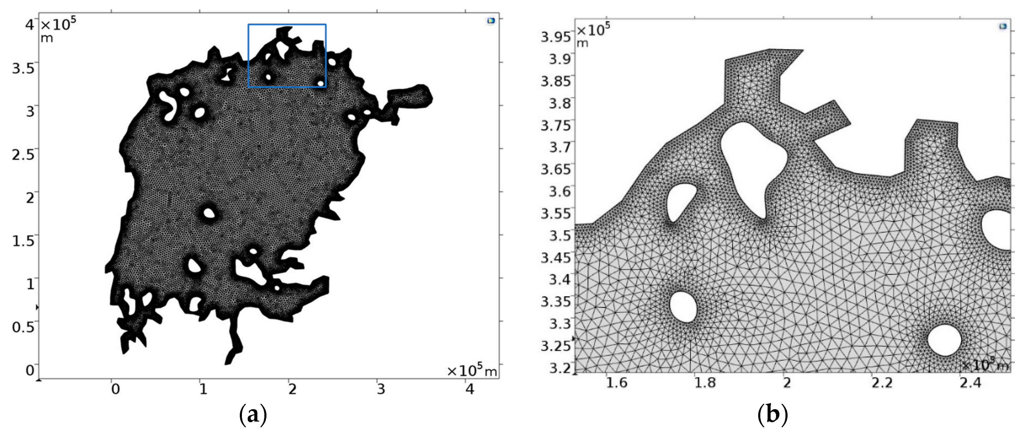Figure 8a shows the generated finite element grid with $67,000$ triangular domain elements and $4000$ boundary elements. There are $107,000$ degrees of freedom $\left(U,V,\zeta \right)$.

Finally, COMSOL assembles and solves the discretized problem. Non-linear equation solvers have access to exact derivatives computed by symbolic manipulation. Sequences of steps created by geometry, mesh, studies, and solver settings, can be recorded to re-compute the problem after modification and to visualize the results.

5. Results and Discussion

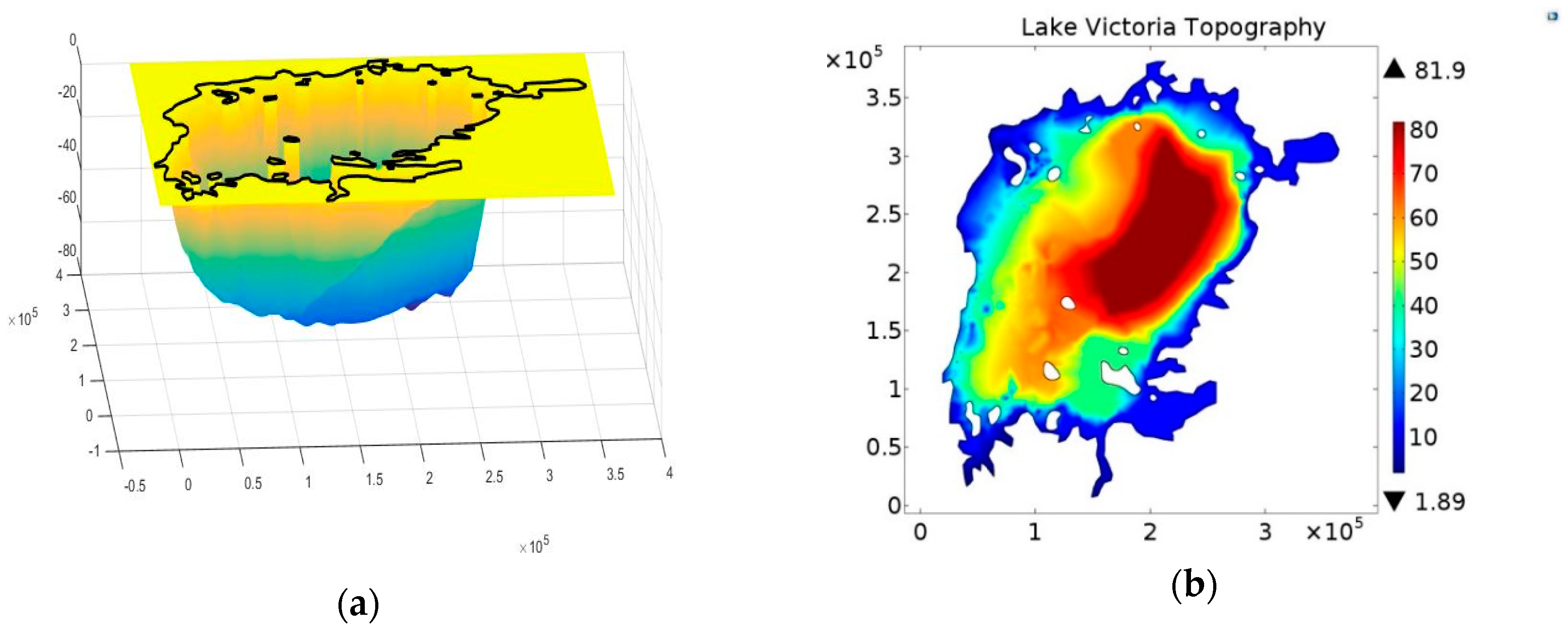
5.1. Lake Victoria Topography in Matlab and COMSOL

The model bathymetry was compiled from several sources and merged as described in Section 3.2. The final geometry based on the iso-depth curves, including islands, plus the NaFIRRI data is shown in Figure 9 as a shaded geometry of the topography of the whole lake with depth (see also Figure 4). The governing equation under PDE solver in CM adopted the SWEs method for the 2D Lake Victoria model.

In the regional flow model analysis, the mass conservation and momentum equations were integrated with respect to the depth. In the initial stage, flow analysis was defined by initial values under initial boundary conditions and boundary values defined by river discharges under DBC. Initial values initially adopted three dependent variables (velocity, U and V; reference water level, zeta) that could serve as an initial guess of water flow analysis. DBC adopted river discharges, which prescribe the lake flows for whole lake areas. The simulations shown here used Neumann conditions to guarantee conservation of water volume. Figure 9 shows that the lake’s bathymetry is steeper in the east than in the west.

Figure 9a lake bathymetry steps down from north to south toward the deepest point (80 m, Tanzania) in the basin. Figure 9b shows that both data and boundary conditions are fixed very well and water flow goes over the lake without encountering a barrier. The two topographical models were used to perform water flow analysis of Lake Victoria, with the two main discharges considered being the Kagera river, which is the main river inflow to Lake Victoria, and the other being the Nile, which is the only outflow from Lake Victoria.

5.2. Lake Hydrodynamics

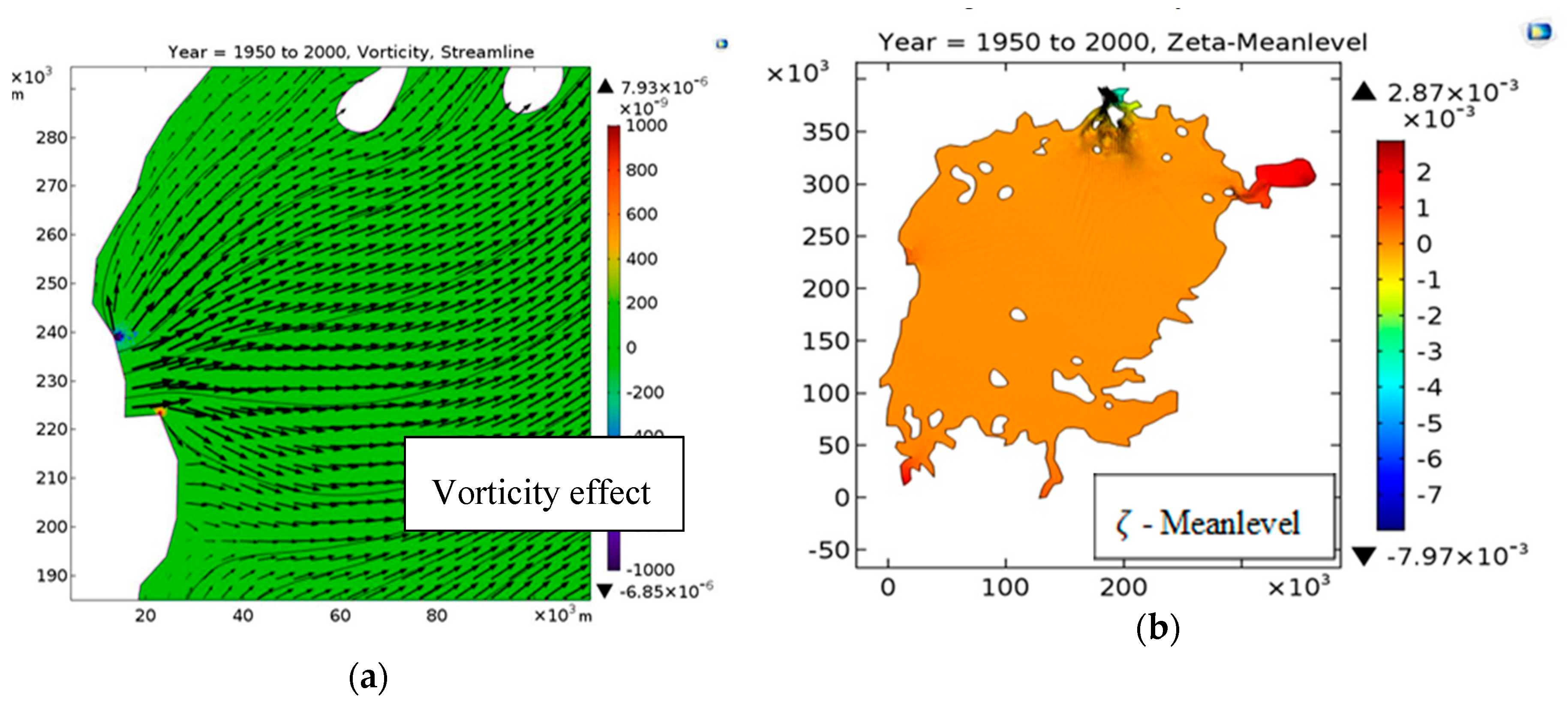
The simulation used monthly averages from 51 years of WRMA data [44] on precipitation, evaporation, inflows, and outflows. The situation in 2000 is presented in Figure 10. The initial data in 1950 are unknown and were set to still water and vanishing wave height, with flux boundary conditions applied to the whole boundary. The outflow boundary conditions allow a steady-state conditions, which is discussed in Section 5.4 below. Note that the shorelines are fixed, and thus do not change with the water level, so the choice of reference height is arbitrary.

The streamlines in Figure 10 show a well-ordered flow from Kagera toward the outflow with no indications of re-circulatory regions. It is indeed close to a flow with vanishing vorticity, $\omega =U_y-V_x$, as substantiated by the vorticity plot.

This is to be expected, since the flow starts from still water, and the gravity driving force is irrotational. The artificial viscosity diffuses vorticity created by its sources: The bottom friction and the weak singularities at the boundary points between inflow and no-flux shore portions. The latter shows up as small red and blue regions, i.e., positive vorticity on one side of the tributaries, and negative on the others (Figure 10a). The influence of (artificial) viscosity and bottom friction was analyzed using Equations (9)–(14), where vorticity ω is the curl of the 2D velocity field:

$$\nabla \times \left(U{\mathit{e}}_x+V{\mathit{e}}_y\right)=\left(U_y-V_x\right){\mathit{e}}_z=\omega e_z$$

(9)

The curl of the momentum equations produces:

$${\omega }_t+\left(\mathit{U}·\nabla \right)\omega +\left(\nabla ·\mathit{U}\right)\omega =-\omega C(\dots )\left|\mathit{U}\right|+\nabla \left(C(\dots )\left|\mathit{U}\right|\right)\times \mathit{U}+{\mathit{\nu }}_{\mathit{A}}{\nabla }^2\omega$$

(10)

$$\omega \left(t=0\right)=0$$

for a case with ${\upsilon }_A$ constant.

The flux boundary conditions are:

$$\mathit{n}·\left(h\mathit{U}-{\nu }_A\nabla \zeta \right)=Q:h\mathit{n}·\mathit{U}-{\nu }_A\partial \zeta /\partial n=Q$$

(11)

$$\mathit{n}·\left({\nu }_A\nabla U\right)=0:n_x{U}_x+n_y{U}_y=0$$

(12)

$$\mathit{n}·\left({\nu }_A\nabla V\right)=0:n_x{V}_x+n_y{V}_y=0$$

(13)

For simplicity, rotate the coordinate system so $x$ is normal and $y$ is tangential:

$$hU-{\upsilon }_A{\zeta }_x=Q$$

(14)

$$U_x=0$$

$$V_x=0$$

$Q$—the net flux is piecewise constant in the model, zero except at tributary mouths. If artificial viscosity at the shore is neglected, the first equation guarantees that $U$ is also piecewise constant, hence, $U_y=0$ except at the jump points of $Q$, the tributary corners. It follows that the boundary conditions make $\omega =0$ on the whole boundary except at tributary corners.

Thus Equation (11) is a diffusion–convection equation for ω with vanishing initial data and, in the sense explained above, vanishing boundary values. It follows that only the term $\nabla \left(C(\dots )\left|\mathit{U}\right|\right)\times \mathit{U}$ in the bottom friction model produces vorticity, and then only the variation of the bottom friction factor C.

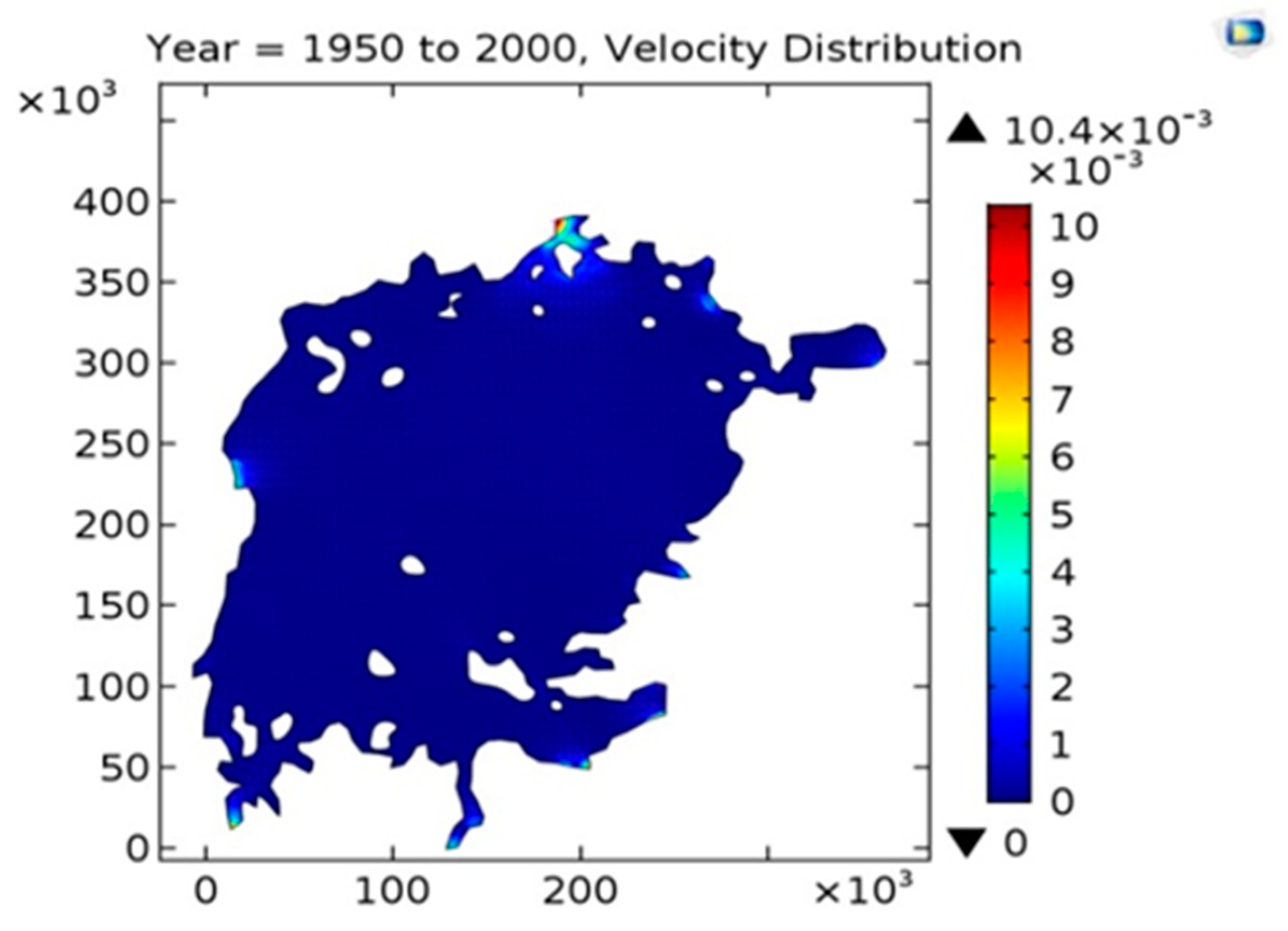
5.3. Long-Time Simulations

The simulation over fifty years over has daily measurement as data. The interest here is to show mean flow patterns as revealed by time-averages, and a month was chosen as a suitable averaging period. Thus, monthly averages of inflow and outflow, precipitation, and evaporation were used as data. The timescale of the driving function was then in the order of a month instead of a day. It has been seen that the mean water level was reproduced faithfully, which is only a circumstantial evidence of overall accuracy. The mean flow velocities (Figure 11) were very small overall at <1 cm/s, so the Froude number was extremely small, and the wave height excursions were at most a few centimetres $\left(\mathrm{cm}\right)$. Mean water level changes in the order of $1\mathrm{m}$ were also small compared to the mean depth of the lake. This means that the model was close to linear and time invariant, which suggests computing the averaged solution as the solution with average driving functions.

The accuracy of the simulation model can be called into question since the driving data were low-pass filtered, and the time-steps used were larger than the travel time for a gravitational wave across the lake. The discretised shallow water model has much faster dynamics, with time-scales $\Delta /a$, O (100 s), where the gravity wave speed is $a=\sqrt{gh}$. The time-stepping is performed by backward differentiation formulas that damp solution components corresponding to stable poles even with large imaginary parts. It follows that using low-pass filtered data and large time steps compared to the fast internal dynamics will damp the fast modes of the system to produce a solution that is closer to the low-pass filtered exact solution.

5.4. Outflow Boundary Allows a Steady-State Condition

Inflow boundary conditions specify the amount of water entering the lake in measured quantities. A “natural” outflow boundary condition, however, should allow an accurate simulation to achieve a steady water level, if inflows are constant. Data on both inflows and outflows are available, and can be applied as boundary conditions. It could be argued that the outflow should react to the lake water level such that increasing levels increase the outflow. A Jinja power station regulates the lake outflow, so other signals influence the actual outflow. Two candidates are discussed here for “natural” outflow conditions: The weir condition (see Section 5.4.1) and a linear outflow condition (see Section 5.4.2) fitted to historic data. Both give well-posed steady-state solutions.

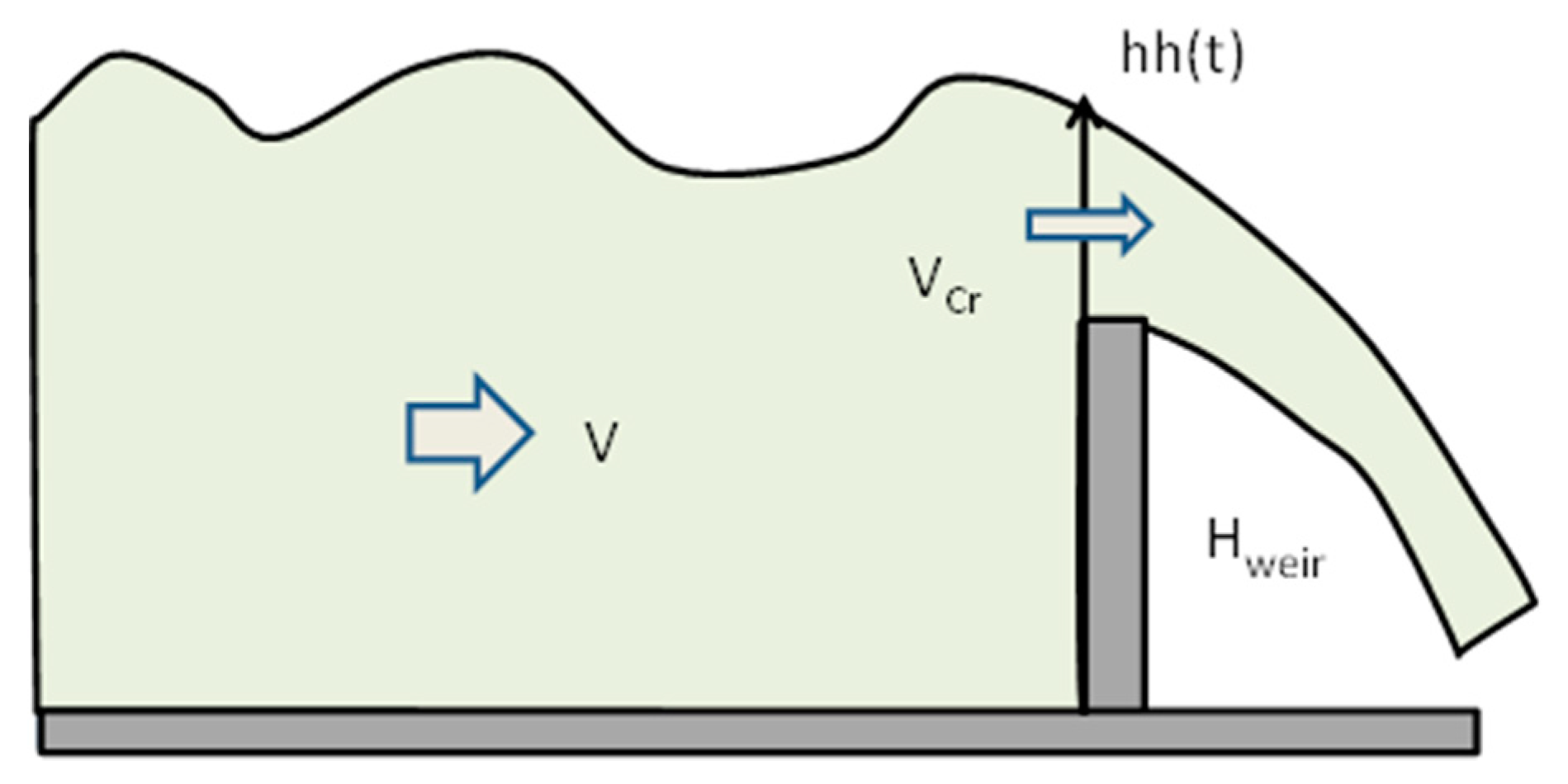
5.4.1. Weir Boundary Condition (WBC)

The WBC model outflows as if it were flowing over a weir of a given height. This approach is strictly applicable only when the upstream flow is steady and subcritical and is unsuitable for rapid variation in proximity of the weir [45,46].

The weir condition expresses that the flow over the weir at the crest is exactly critical (see Figure 12):

$$V=\left(1-H_{weir}/hh\right)V_{Cr}=\left(1-H_{weir}/hh\right)\sqrt{g\left(hh-H_{weir}\right)}$$

(15)

and $V=0$ if $hh<H_{weir}$. The flow increases non-linearly with water level and WBC sets a definite steady-state water level, when inflow, evaporation, and precipitation are constant.

5.4.2. Linear Outflow Conditions

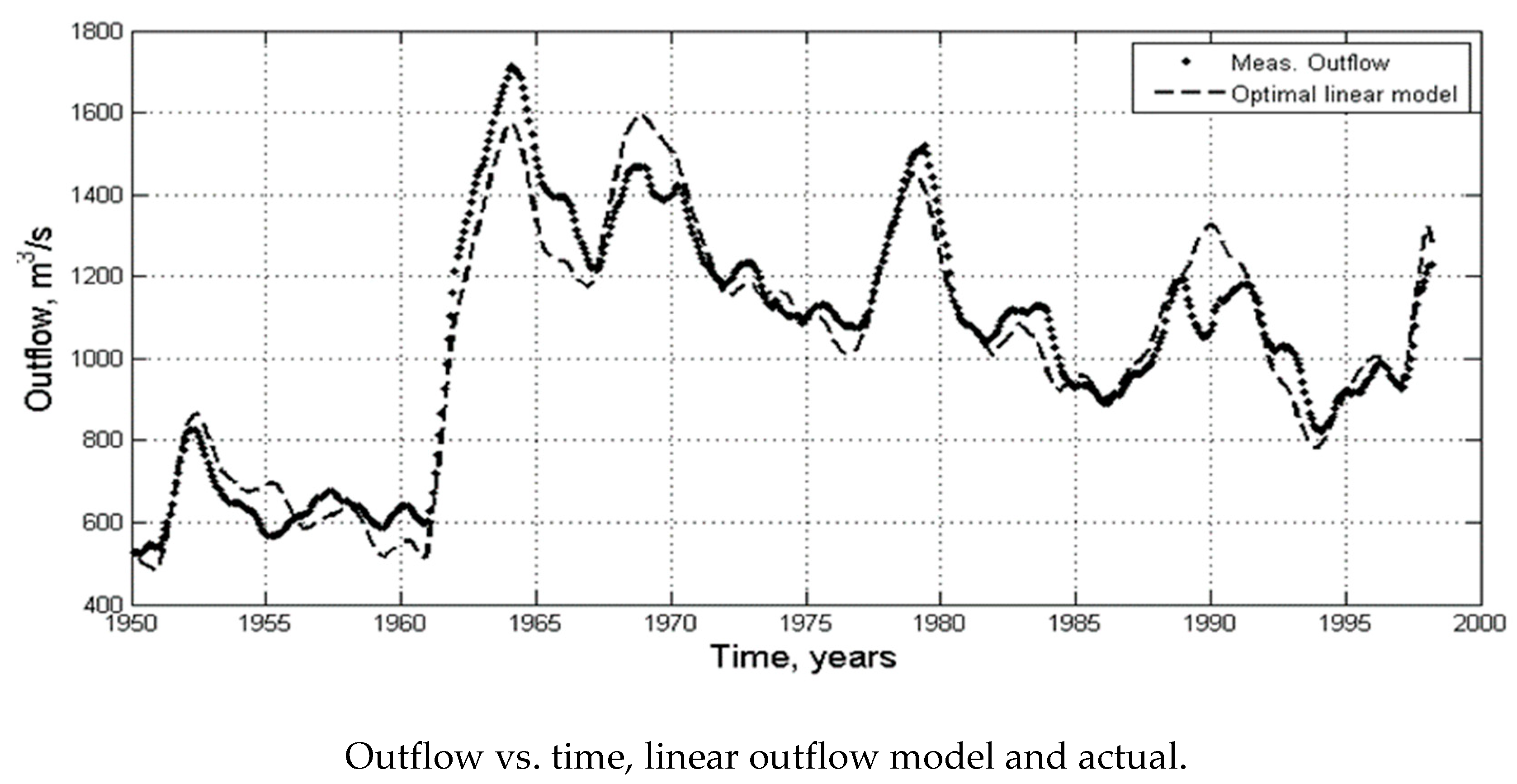
In view of the simplicity of the model (Figure 13), the agreement was excellent. One issue is that the Nile outflow should react primarily to the local water level rather than the mean water level. This effect is mitigated by two factors:

• Net precipitation is a dominant source and is assumed to be homogeneous over the whole lake area;
• the travel time for a gravitational wave across the lake, assuming a mean depth of 60 m, is around $3.5$ h. Thus, water level differences would equalize over the lake in a much shorter time than a month.

The NaFIRRI measured data contain discharge from the tributaries (In), the outflow at Jinja (Out), precipitation (Precip) and evaporation (Evap). The data admit an estimate of the mean water level h, as shown in Equation (16):

$$\mathit{Area}·\mathit{dh}/\mathit{dt}=\mathit{In}+\mathit{Precip}-\mathit{Evap}-\mathit{Out}$$

(16)

where, the lake area is assumed constant in time. In order for the SWE simulation to allow a steady solution, the outflow should increase with the water level. The non-linear weir outflow condition does that, however, even simpler models may give a good fit to the observations. The simplest choice for an outflow condition is a linear relationship to water level, measured from a reference level:

$$Out(t)=Ch(t)$$

(17)

Thus, to find the initial water level $h(0)$ and the constant $C$:

$$Area·dh/dt=In+Precip-Evap-Ch$$

(18)

$$h(0)=h0$$

Such that the outflow $Ch(t)$ matches the measured outflow $Out(t)$ as closely as possible. The optimal values were found by solving the nonlinear least squares problem where $t_j=j\Delta t,j=0,1,\dots$ gives a simple time-implicit discretisation of the ordinary differential equations (ODE):

$${}_{h_0,C}^{\min }{{\displaystyle \sum \left(Ou{t}_j-C{h}_j\right)}}^2$$

(19)

So that:

$$h_j=h_{j-1}+\Delta t/Area\ast \left(In\left(t_j\right)+Precip\left(t_j\right)-Evap\left(t_j\right)-C{h}_j\right)$$

(20)

$$h(0)=h0$$

The agreement with measured outflow was excellent (see Figure 13). Short time discrepancies between the linear approximate model and the measured outflow are seen at 1966, 1969 and 1990 (Figure 13). This shows that regulation at the power station in Jinja was active, acting more on input than on water level. Overall, the linear model agreed with the “agreed curve” [47] for outflow regulation from water level, so the good fit was to be expected if the Jinja regulation followed the agreed curve.

5.5. Water Level Validation

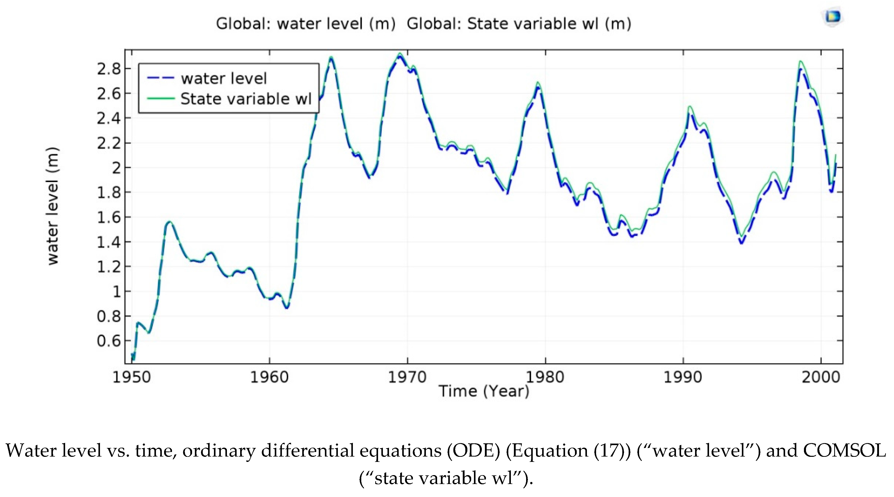
The simulation of Lake Victoria’s water level was based on fifty one years of data for precipitation and evaporation over the lake, and river inflow and outflow.

Generally, lake water-level regimes are influenced by climate variation, lake hydrology and land uses. Lake Victoria’s water level has changed significantly in ways that have puzzled researchers. From 1900 to 1961, the lake’s water level was different from that in the 1961–2000 time period (Figure 14), which also shows that the result of the water balance model (Equation (18)) agrees with the mean water level computed by CM and demonstrates its conservation property.

The mean water level rose rapidly by about 2.8 m from 1960 to 1965, from 1968 to 1971, and from 1998 to 2000. As a result, the increased water level seen in the peaks of 1961–1964, 1968–1971 and 1998–2000 in Figure 14 are also noticeable in the discharge.

6. Conclusions

A systematic method was developed in Matlab for lake bathymetry and lake flow was analyzed with a depth-integrated shallow-water free-surface numerical model in CM. Depth data from old depth soundings given as iso-depth curves were merged with modern echo-sounding data received from NaFIRRI. Kriging interpolation was unable to produce a sufficiently smooth lake topography. The DACE toolbox with Delaunay triangulation that created the Kriging interpolation was used, followed by an isotropic Gaussian filter. Discrepancies in the lake shoreline were rectified by a bilinear transformation of the old shoreline.

The successful bathymetry model was used in a vertically integrated flow model along with measured inflow, outflow, rainfall, and evaporation data. The shallow water model analyzed mean flows and predicted mean water levels reasonably well. The mean flow velocities were very small overall, and the mean water-level changes were also small compared to the mean depth of the lake. This means that the model was close to a linear, time-invariant model. This enabled computation of the low-pass filtered time series of water levels as the result of low-pass filtered input data, providing fifty-one year simulations. The mean water level was reproduced faithfully, offering only circumstantial evidence of overall accuracy. A linear outflow boundary condition achieved a significant correlation with measured outflow. The measured water level agreed reasonably well with the computed water level, which is crucial for lake numerical model validation in CM.

Software and data sources: The Comsol Multiphysics [48] software has many model libraries to focus on different areas, however, no special model libraries for surface waterbody analysis. The bathymetry, inflow/outflow, and precipitation/evaporation data for the model were obtained as described above: From our collaborators at Makerere University, Uganda, Water Resources Management Authority (WRMA), Kisumu, Kenya and Lake Victoria Basin Commission (LVBC), Kisumu, Kenya. Access to the data was granted by the sources referenced. Matlab was used for bathymetry data processing.