1. Introduction
Modern interest in wind energy emerged after the first oil crisis in the 1970s, and a concerted effort followed to develop viable utility-scale wind energy technologies. The megawatt wind turbine debuted in 1998, and by 2010, wind turbines in the 2 MW and 5 MW classes became the standard of onshore and offshore applications, respectively. An even larger 10 MW wind turbine has been designed and tested offshore [
1]. The introduction of a 10 MW–20 MW wind turbine with rotor diameter over 200 m was also planned [
2].
Wind turbines operate in the eddies and gusts generated by wakes from upstream turbines and atmospheric turbulence. The highly unsteady flow over the rotating blades is characterized by large transient changes in angle-of-attack, laminar-turbulent transition, flow separation and reattachment, and dynamic stall. Most experimental studies use model-scale wind turbines due to the high cost of full-scale testing, and past numerical studies have been conducted via multiple approaches of different fidelities. Rotor-scale large-eddy simulation (LES) of the blade boundary layer for a full-scale wind turbine still exceeds the state-of-the-art [
3]. Therefore, lower-fidelity models such as the actuator-line model [
4,
5] are often used instead. Unfortunately, lower-fidelity models are incapable of predicting the aforementioned unsteady flow phenomena. The uncertainty of performance and loads predictions in the wind energy industry remain high compared with conventional energy sources.
While the LES of full-scale turbulent rotor flow is still too expensive for most practical problems, the next order of fidelity, Reynolds-averaged Navier Stokes (RANS) models cannot replicate many complex flow features. As such, the RANS approach currently falls short in precisely predicting the shaft torque at stall, as laminar/turbulent boundary layer transition and flow separation have both been shown to have first-order effects on blade aerodynamics predictions [
5]. Full-scale computational fluid dynamics (CFD) studies have shown that increasing RANS fidelity for separated flows and wake regions by employing detached-eddy simulation (DES) can significantly improve predictions of blade torque near stall compared with RANS [
6,
7,
8], and the application of the hybrid RANS/LES model yielded nearly identical solutions compared with RANS at low wind speed.
One of the major difficulties in full-scale CFD is the large diversity of both temporal and spatial scales in wind plant operation conditions. In the atmospheric boundary layer, the energy-containing motions are on the time scale of minutes and the length scale from 10 to 1000 m, while the attached blade surface viscous boundary layers have time scales on the order of milliseconds with length scales of importance down to 10 μm (e.g., see [
3]). Thus, neither RANS nor LES models perform well across the entire time/space range of the full-scale problems.
The hybrid RANS/LES model in this study is based on a correlation-based four-equation RANS transition model, which integrates two local-variable transport equations with the shear stress transport (SST)
turbulence model framework [
9]. It is capable of capturing natural, bypass and separation-induced transitions [
10]. An application of the transition model to a small, full-scale wind turbine in the literature showed improved agreement with experiments compared with RANS and engineering models [
11]. For a wind turbine operating in the wake of an upstream turbine, blades experience large variations in angle of attack; the transition model alone helps capturing the load hysteresis loop in dynamic stall [
12]. A recent study [
13] assessed the effects of blade boundary layer transition inside atmospheric turbulence eddies through blade-resolved simulation and full-scale field experiments. The authors found that the boundary layer separation was closely correlated with the transition locations in off-design conditions, where the blades experienced massive separations and deep stall [
13]. Despite the improvement, however, further development is needed for properly predicting the reattachment process.
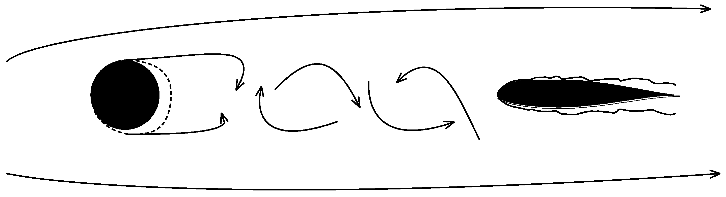
In the current effort, a new surrogate model problem (
Figure 1) is developed; the cylinder-airfoil design encompasses key flow physics such as large-scale, rotational unsteadiness and a transitional boundary layer over an aerodynamic body. A number of past experimental studies involving circular cylinders have focused on various flow problems, including aeroacoustics [
14], spanwise correlation [
15], vortex and wake dynamics [
16,
17], and drag reduction [
14]. The 3D nature of turbulent flow causes phase shift in the spanwise direction, which accelerates the flow structure break-down and turbulent energy cascade [
15]. A cylinder-plate configuration is one of the well-studied wake/body interaction problems, and experimental results have indicated strong correlations between the passage of wake vortices and flat-plate boundary layer dynamics, including the formation of secondary flow structures and transition onset [
16]. Of interest to the wind turbine problem motivating the current work, the spacing between the upstream circular cylinder and downstream plate has a major effect on the dynamic loads on the plate. For instance, when plate is supported so that it is free to rotate around its centerline, the flow-driven oscillations of the plate at small spacings are dominated by the passage of shed vortices from the upstream cylinder, while larger spacings show dominance of self-forcing from wake features shedding off the plate [
18]. It is interesting to note that equilibria, as well as major oscillations around these equilibria, are present for both bluff and aligned plate orientations.
The study on the effect of cylinder wake on a downstream airfoil is of particular interest for our research. The highly-turbulent wake of the cylinder induces transition of the airfoil boundary layer and postpones separation on the airfoil. Past studies found that the attached boundary layer further reduces the vorticity magnitude in the airfoil wake, which improves its aerodynamic characteristics [
14]. Detailed experimental results have been obtained [
17], providing quantitative data for comparison and insights that guide model developments. Leveraging the new insights, we developed a novel hybrid RANS/LES approach which includes transition modeling, and, thus, has the advantages of both resolving the energy-containing turbulence structures generated upstream of the blade and also improving the fidelity of physics modeled in the blade boundary layer region. Some preliminary computational results of circular cylinder flow and airfoil boundary layer were published previously [
19].
The objectives of this study include: (1) design of a small-scale surrogate wind-tunnel model using a collaborative CFD-EFD (experimental fluid dynamics) approach, capturing key flow physics; (2) perform high-fidelity experiments which can provide validation-quality data and guide the development of turbulence models; (3) incorporate the Langtry-Menter 4-equation transition model [
20,
21] into a hybrid RANS/LES framework and validate resulting computational approach; and (4) provide analysis of the results to further our understanding of unsteady transitional boundary layers on wind-turbine airfoils.
Section 2 introduces the design of the surrogate model and its model parameters.
Section 3 presents the turbulence model used in the current study and the corresponding simulation setups.
Section 4 contains simulation results of cylinder flow using the hybrid transition model, also including the comparison with experimental data.
Section 5 is an analysis of the unsteady airfoil boundary layer and comparison between the simulation and experimental results. Finally,
Section 6 concludes the paper.
2. Model Formulation and CFD-based Experimental Design
The aerodynamics of wind plants consists of eddies, boundary-layers, and wakes which fall in a vast range of length and time scales (
Table 1). The full-scale problem is too complicated and computationally expensive for fundamental model development and verification, validation, and uncertainty quantification (VVUQ). A typical study of a 5 MW full-scale single rotating blade in the atmosphere with well-resolved boundary layers requires over 50 million cells and thousands of processors, and each intermediate output at a single time step from the CFD solver occupies over 20 GB of storage [
3]. Therefore, we are motivated to develop a surrogate model.
The current study adopts a complementary CFD-EFD approach, and preliminary simulation data are used to guide the experimental design. The experimental data is used for turbulence model validation purposes, while the comparison and analysis of numerical and experimental data lead to the fully-described flow physics of the unsteady boundary layer.
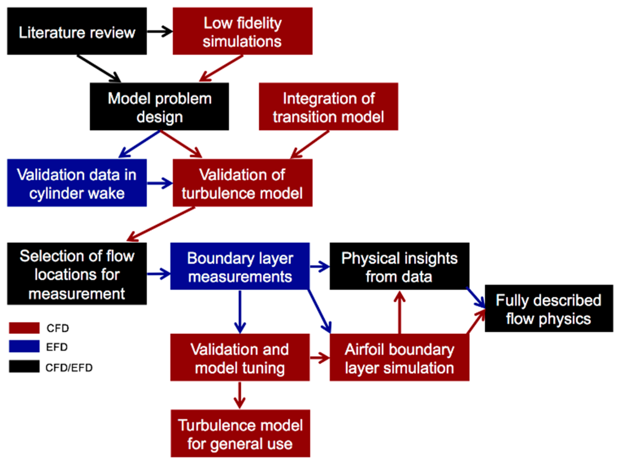
An overview of the experimental and numerical procedure is shown in
Figure 2. The flow chart consists of red blocks for numerical work, blue blocks for experimental work and black blocks for joint efforts. All the experiments and corresponding analysis were conducted by co-author D.R. Cadel and the details can be found in the article by Cadel et al. [
22].
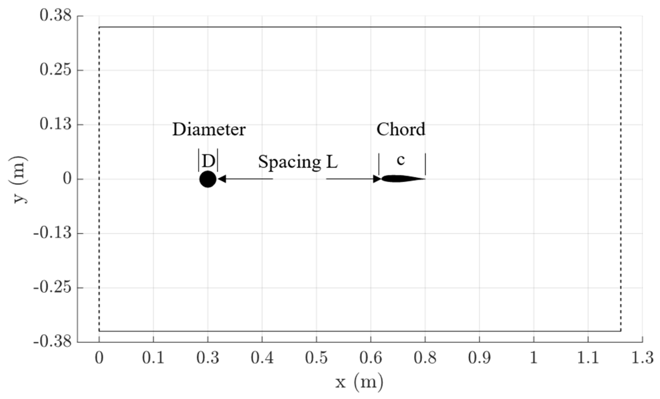
The surrogate model in our study consists of a modified NACA 6-series airfoil [
23] embedded in the wake of a circular cylinder, which is used as the surrogate atmospheric turbulence generator.
Figure 3 is a sketch of the experiment setup in the test section, the freestream velocity is at
and turbulence intensity
The diameter of the circular cylinder is
, and the airfoil chord length
c = 10.2 cm, which corresponds to
and
.
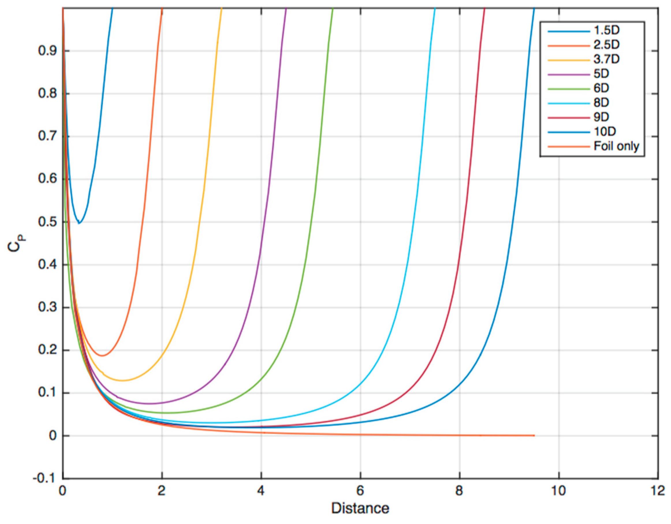
The key parameter of this surrogate model is the spacing
L from cylinder center to airfoil leading edge, in order to minimize the direct effects on unsteady boundary layer physics from the upstream cylinder, the airfoil is placed outside the immediate wake of the cylinder. Various spacings from
up to
were test using the potential flow solver in OpenFOAM (Version 3.0), and the pressure recovery curves are plotted from cylinder rear stagnation point to airfoil leading edge as shown in
Figure 4, as the airfoil moves further than 9
downstream the pressure recovers to near freestream level (
) at
. The furthest airfoil position is also limited by the experimental equipments, e.g., the total length of the test section and particle image velocimetry (PIV) camera blockage from test section supporting brackets, the spacing is finally decided at
, i.e.,
. Flow conditions and model parameters are summarized in
Table 2.
The validation experiments are conducted in Virginia Tech’s 0.7 m blower type subsonic wind tunnel with a closed acrylic-walled test section. Two laser/camera systems were used to acquire PIV data. For the cylinder wake measurements and time resolved boundary layer measurements, a diode-pumped Nd-YLF frequency doubled 527 nm laser (Photronics Industries International, Inc., Ronkonkoma, NY, USA) was used, with a maximum pulse energy of 70 mJ at 2920 Hz. Photron Fastcam SA-1 cameras with 1024 × 1024 pixel sensors were used with this laser. For the non-time resolved airfoil cross-section measurements, an EverGreen 200 Nd:YAG laser (Quantel, Bozeman, MT, USA) was used with a maximum pulse energy of 200 mJ at 4 Hz. Two Imager pro X 4M double shutter charge-coupled device (CCD) cameras (LaVision, Ypsilanti, MI, USA) with 2048 × 2048 sensor size were used with this system. Due to low stereoscopic sensitivity of the spanwise component in the boundary layer measurements only the in-plane velocity data are analyzed. DEHS oil (mean diameter 1 μm) was used for cylinder wake measurements, and a smoke consisting of 50% pharmaceutical grade glycerin and 50% deionized water (0.2–0.3 μm diameter) was used for all other PIV data. Seed was introduced immediately downstream of the fan blower, well upstream of the honeycomb grids, and was seen to be dispersed and uniform in the test section. Higher seed density is introduced upstream for the airfoil unsteady boundary layer measurements due to high magnification boundary layer planes.
Owing to the limited spatial resolution, the uncertainty in PIV data is estimated at 1% of the velocity magnitude [
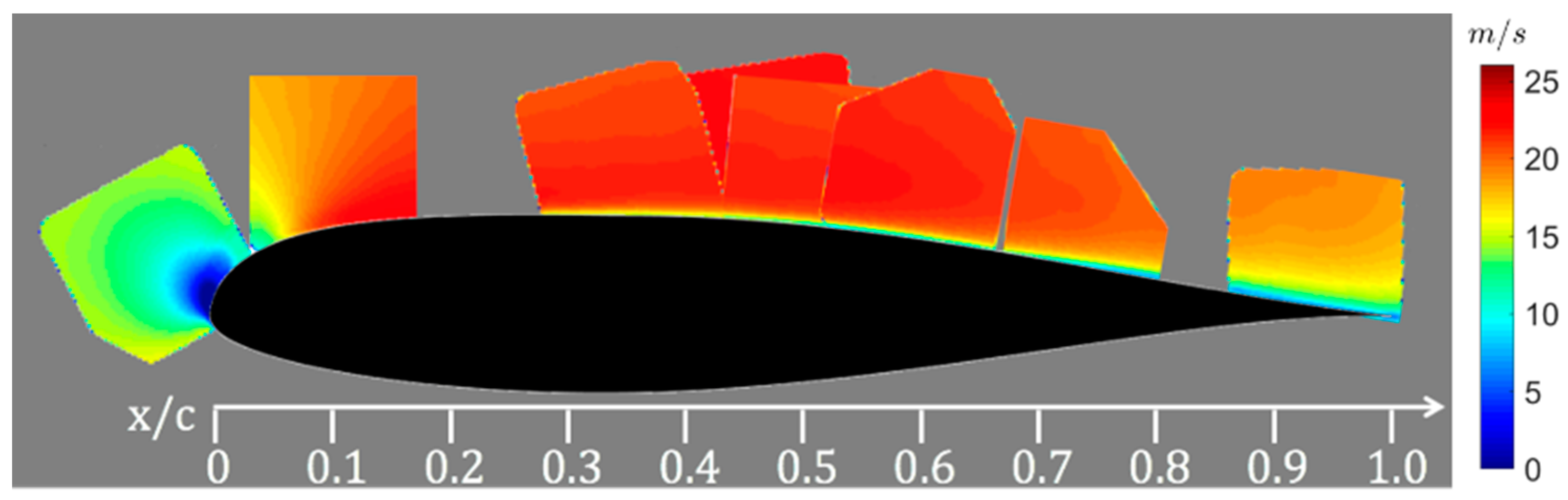
17]. Both the airfoil and cylinder models are chrome-plated in order to mitigate laser flare during PIV testing. Flow field data is acquired in both the cylinder near wake and on the suction side of the airfoil. Extra effort is made to obtain airfoil near-surface measurements (see the airfoil near-surface planes depicted in
Figure 5). For the cylinder wake measurements, 10,658 total realizations were acquired over four runs, and were subsequently normalized using the measured plenum pressure in order to combine sets for analysis. Airfoil measurements over the full chord were acquired with 2000 realizations for each inflow case. For the boundary layer profile measurements, 2728 images were used for the steady inflow case at each station, and 5456 images were used for the periodic inflow case at each station. A 40 mm × 40 mm field of view with grid spacing of 0.6 mm was acquired for the cylinder wake measurements. Airfoil measurements over the full chord had a grid spacing of 0.5 mm. For the boundary layer profile measurements, 15 mm × 15 mm fields of view with grid spacing of 0.23 mm. Many further details of the experiment are discussed in past published works [
22,
24].
Although the airfoil Reynolds number is two orders of magnitude lower than full-scale problem, and the imposed unsteadiness from upstream cylinder is much higher in frequency, our surrogate model still captures key features of the unsteady physics as seen in full-scale problems. A future experiment at near-full-scale conditions is planned in the Virginia Tech Stability Wind Tunnel (183 cm × 183 cm cross section).
4. Circular Cylinder Flow
Flow over circular cylinder is a well-studied problem, abundant experimental and numerical data is available from low-Reynolds number laminar flow up to supercritical high-Reynolds number turbulent flow. In our test, the circular cylinder Reynolds number , which is in the subcritical flow regime. Cylinder experiences laminar separation and flow bursts into turbulence inside the shear layer. Alternative vortices are formed from shear layer roll-up and shed downstream with constant Strouhal number. Beyond the subcritical regime, the cylinder boundary layer transition initiates before separation and delays the separation points, which significantly reduces the pressure drag and total drag, thus the named “drag crisis”.
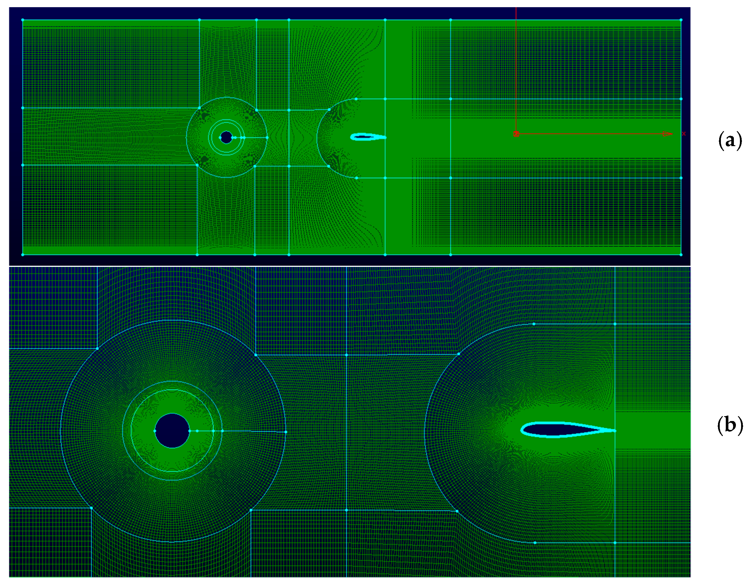
The objective of studying circular cylinder flow is to test the hybrid transition model performance and confirm that we can accurately predict unsteady flow off the cylinder. The spanwise dimension is fixed at
(one chord length), and a grid independence study was conducted using three systematically refined mesh. Grid statistics of the coarse, medium and fine mesh is summarized in
Table 3.
All three simulations use the hybrid transition model as introduced above, same numerical schemes are used to solve the linear system with fixed time step of . The results from coarse mesh predict different flow physics than the other two cases, the boundary layer separates later, which results in higher shedding frequency as seen in supercritical cases. The differences in force and shedding predictions between medium and fine mesh are within . Thus, the medium mesh is adopted in the current study for its performance and moderate computational cost.
4.1. Instantaneous Flow Field
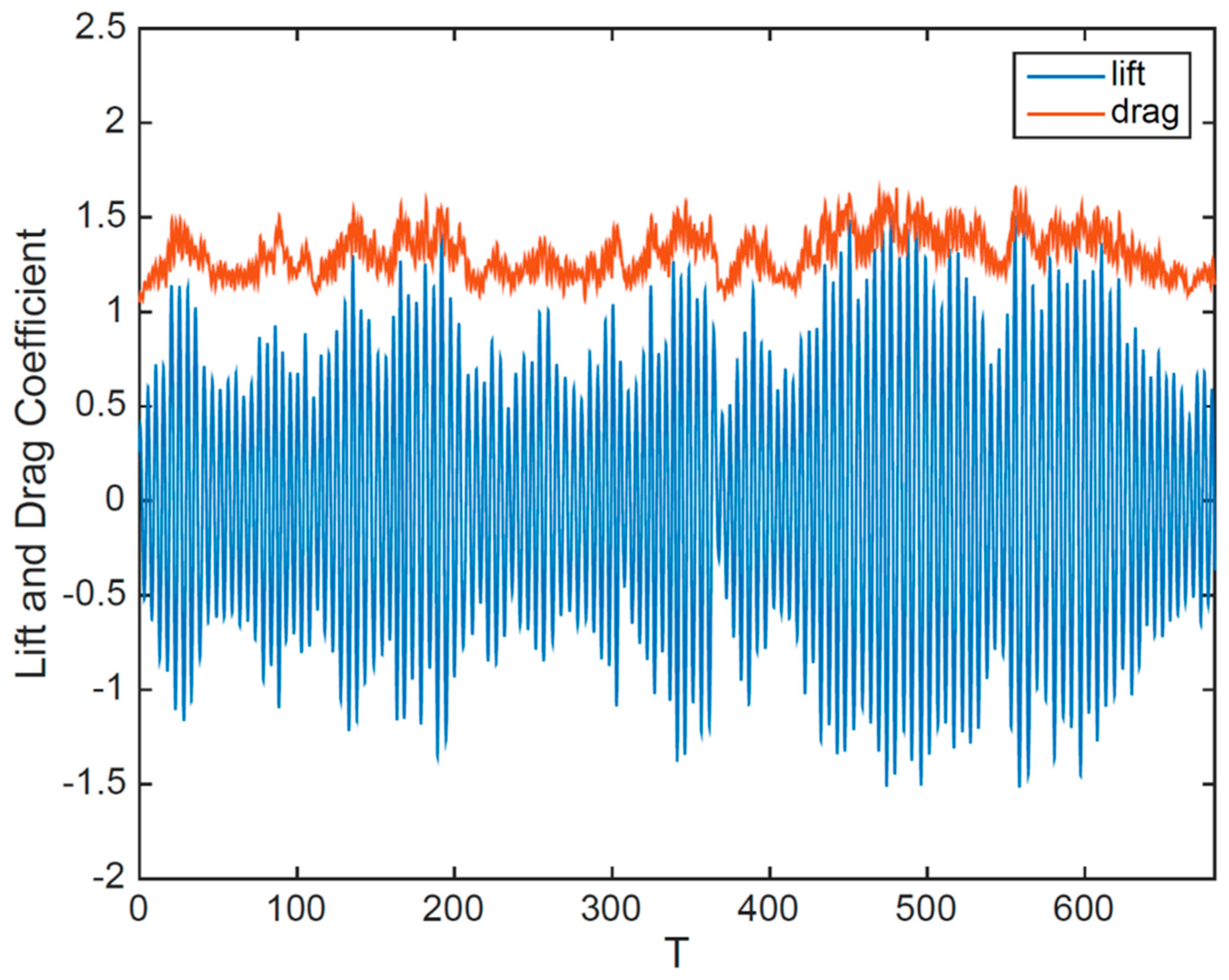
The time history of cylinder lift and drag coefficients are shown in
Figure 7, the mean drag coefficient
and the lift coefficient
averages at 0. Both force coefficients are plotted against the non-dimensionalized time
, i.e.,
equals to
simulation time. The first
history is neglected to exclude any transient effects. The spectral analysis of the oscillatory force on circular cylinder shows a dominant lift force frequency at
, which corresponds to Strouhal number
. The wake shedding frequency from our PIV experiment is approximately
and
. Complied experimental data of
for circular cylinder at Reynolds number around
is in the range of
[
30], the simulation data lies in the middle of the range.
The instantaneous pressure distribution on the circular cylinder shows the front stagnation line oscillates with eddy shedding, which agrees with hot-wire data from experiments [
31]. The separation points on both sides oscillates with amplitude of approximately
with the mean separation angle of
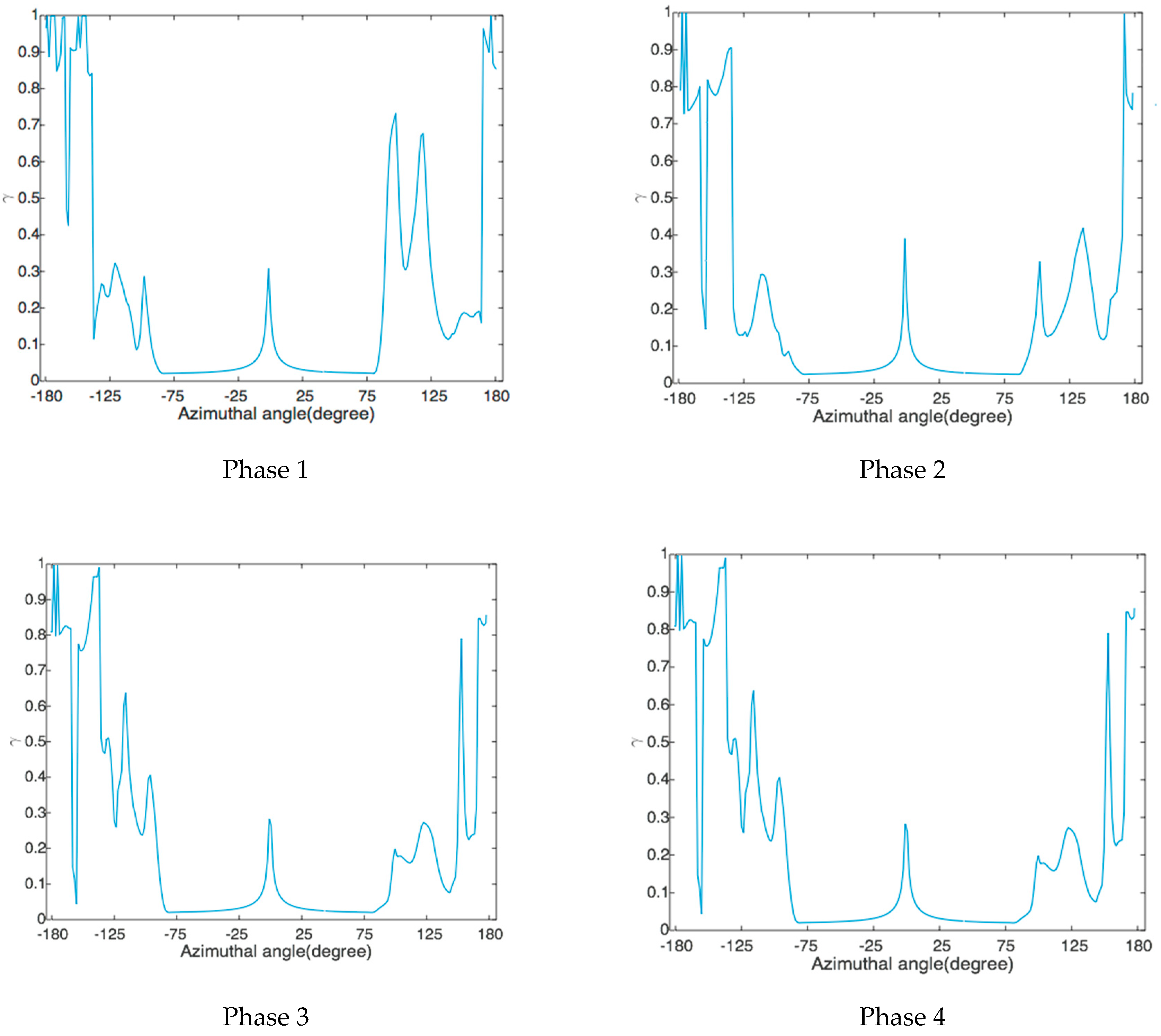
from the front stagnation point. The instantaneous LM intermittency distribution on cylinder is plotted at four phases over one shedding cycle as shown in
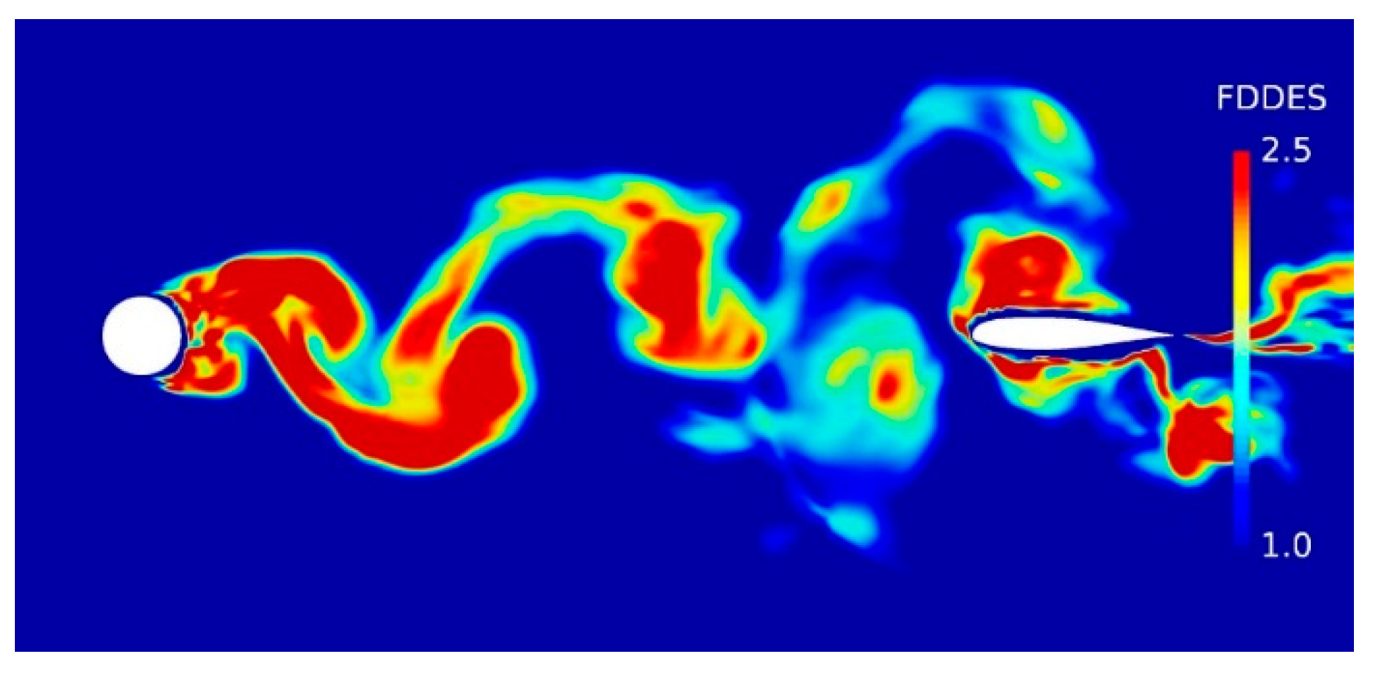
Figure 8. The peak near the front stagnation point is a numerical artifact which is caused by the diffusion of the freestream LM intermittency(
). Between
the distribution of
remains low and steady over the entire shedding cycle and the boundary layer remains laminar. Transition initiates after separation. Various experiments were conducted in the range of subcritical Reynolds number, studies found the separation angle oscillates between
and
from the front stagnation point for circular cylinder of
[
32].
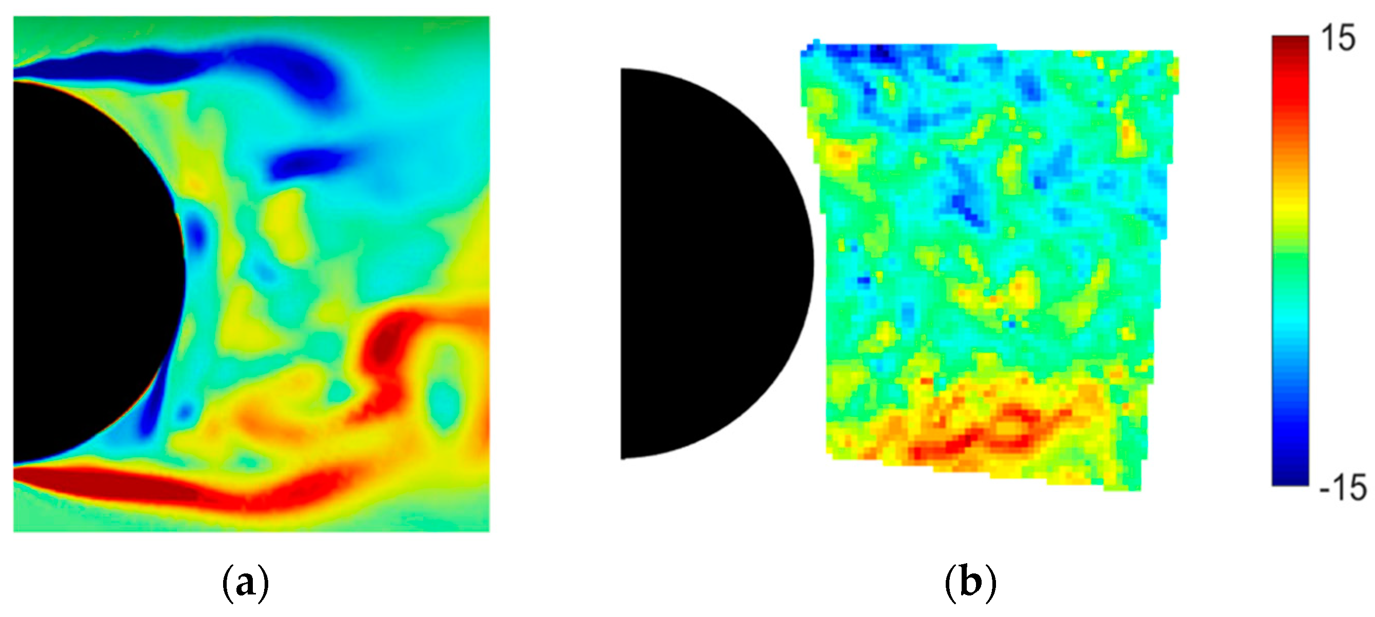
The stability of the shear layer is correlated with the intensity of eddy viscosity. Compared with the experimental data, simulation results predict less stochastic structures in cylinder wake than experiment and the shear layer is more coherent in the streamwise direction (
Figure 9), which leads to longer a recirculation zone in the cylinder wake.
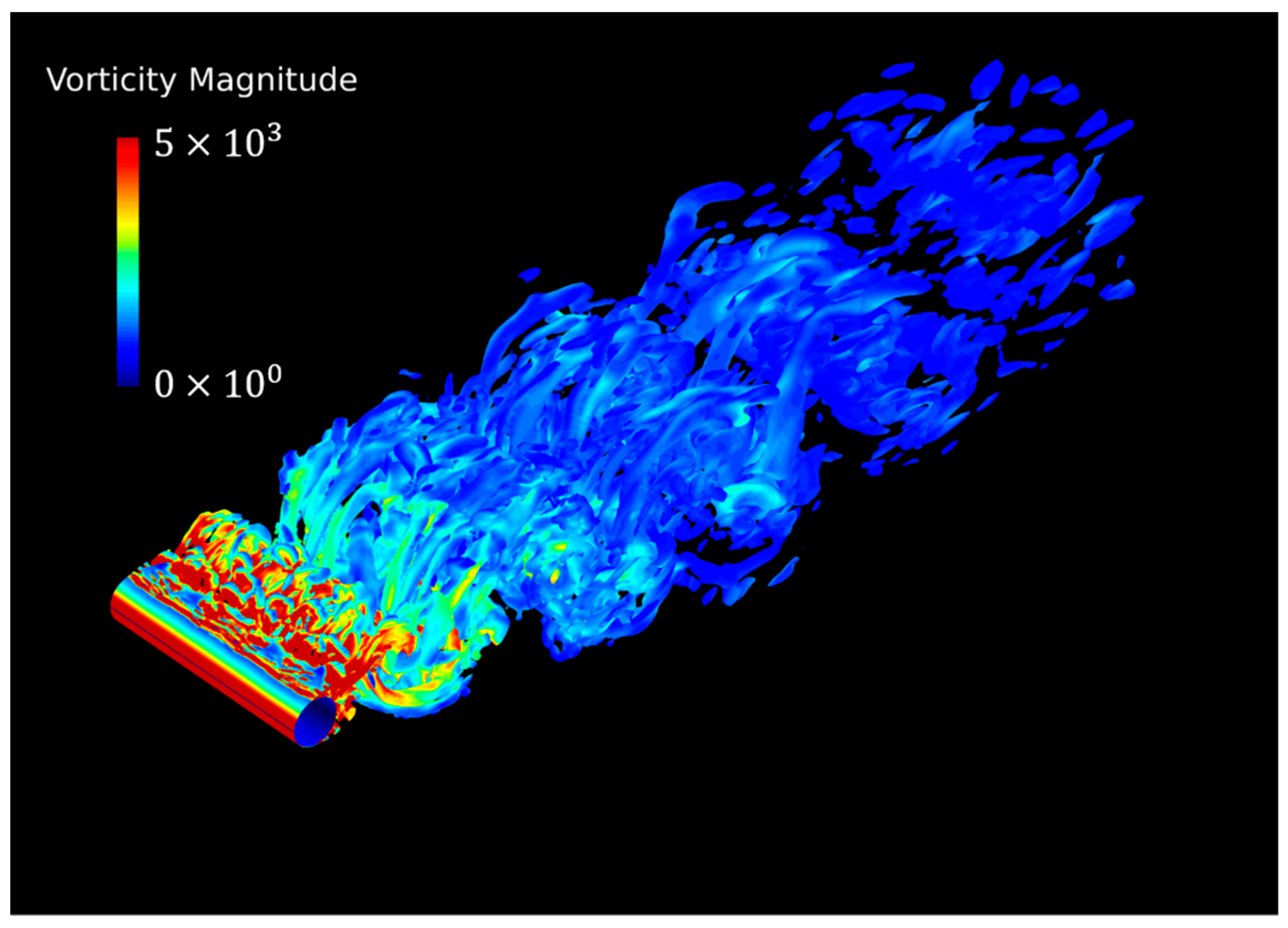
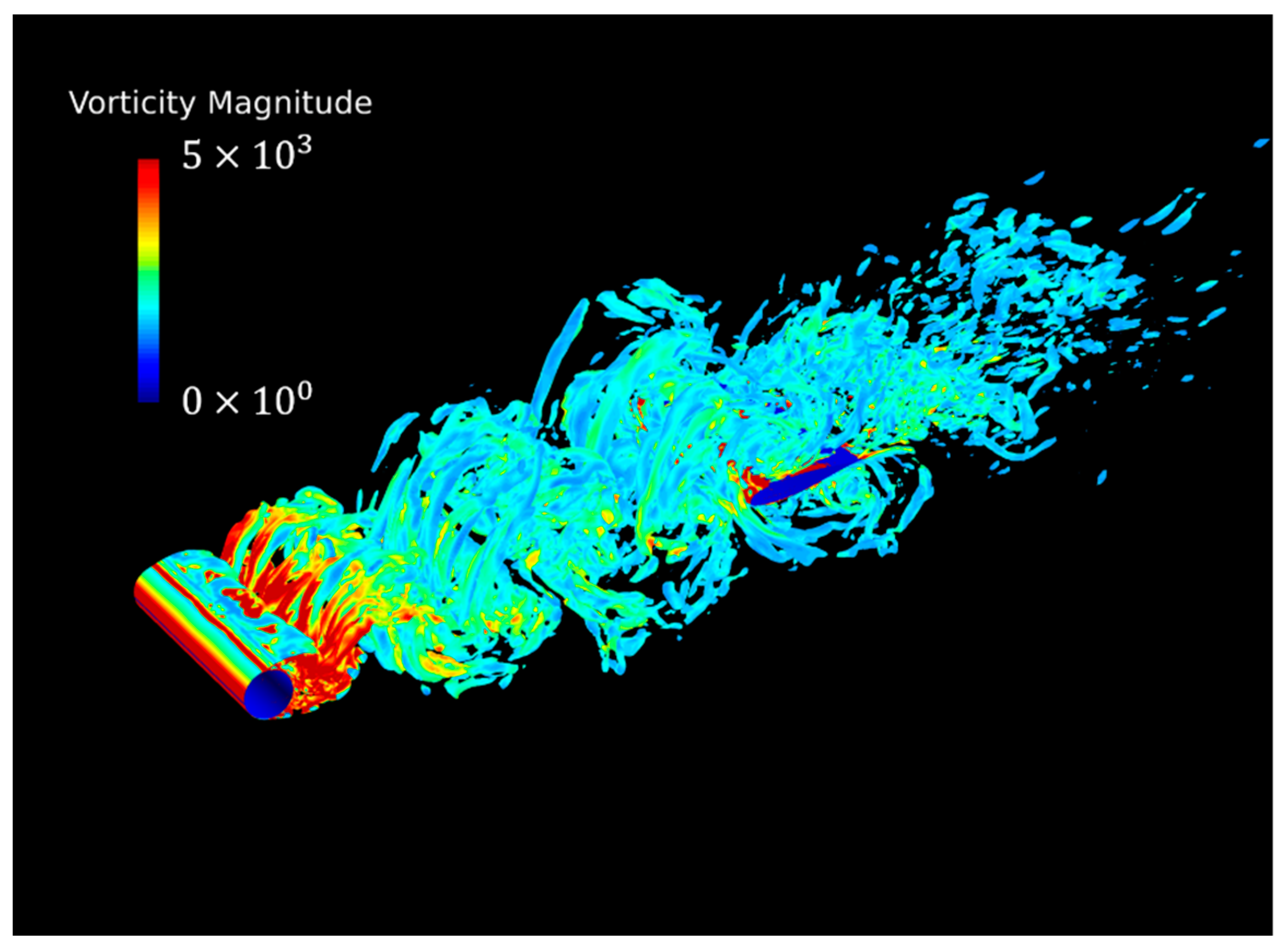
Figure 10 is an example of instantaneous iso-surface of Q-criterion colored by vorticity magnitude; it outlines the shedding vortices as they travel downstream and diffuse outwards at the same time. The spanwise band on the circular cylinder right before separation indicates a uniform separation position. Extensive experiments found significant effects of cylinder aspect ratio on the correlation length in low Reynold number regimes (
). This dependency diminishes beyond
and correlation length
[
33].
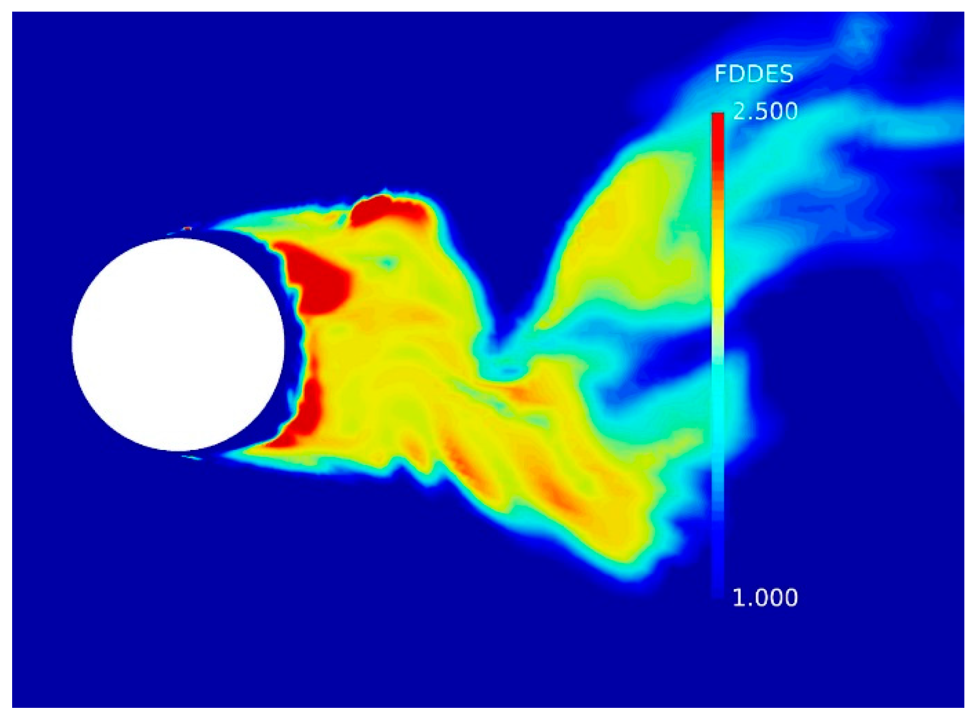
The blending of the hybrid model is fulfilled by the blending function , which is directly multiplied to the destruction term in the TKE equation (Equation (4)). Compared with the RANS formulation, modeled turbulence is reduced in all regions of .
Inside cylinder boundary layer,
remains value of 1 (
Figure 11), which preserves the boundary layer to RANS, it is essential for the hybrid model to work as desired since the boundary layer mesh cannot support resolved turbulence structures. Outside the cylinder wake, turbulence is close to freestream level, and the turbulence model operates in RANS mode, hence
.
4.2. Mean Flow Field and Flow Statistics
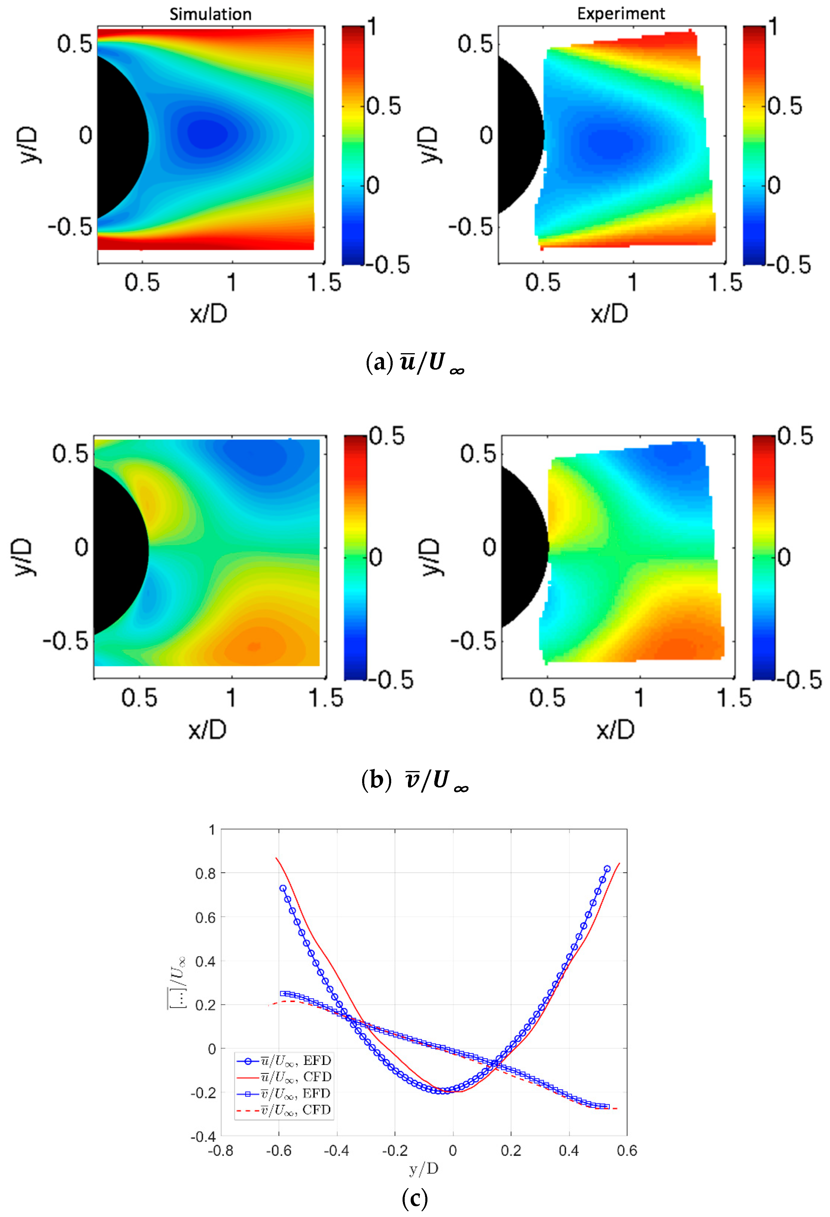
The comparison of mean velocity components
and
in cylinder wake up to
downstream is shown in
Figure 12. The shape of PIV interrogation widow limits the acquired data in a rectangular region that is tangent to the cylinder surface, all data is normalized by the freestream velocity
. The numerical prediction of the length of recirculation zone and width of the wake as seen in
Figure 12a are within
difference compared with experimental data. A quantitative comparison between EFD and CFD results for the stream-wise and transverse velocities is presented in
Figure 12e. The experimental results exhibit a slight asymmetry in the stream-wise velocity profile, which deteriorates the comparison; however, otherwise, the quantitative agreement of the results is satisfactory.
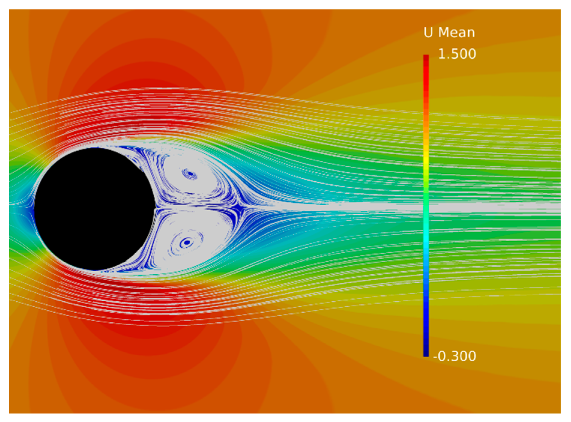
The streamlines of mean streamwise velocity from simulation in
Figure 13 shows the recirculating flow extends to
downstream of the rear stagnation point, and the width of the wake, which determines the eddy shedding frequency, is approximately
. The transverse velocity component
is antisymmetric about the center wake line (
Figure 12b), as expected for transverse mean flow in a plane wake, and the main vortex formation region is centered at
downstream of the cylinder center. Another notable feature in
Figure 12b is the small counter-rotating region near cylinder rear surface, which was also captured by experiments as separation bubbles.
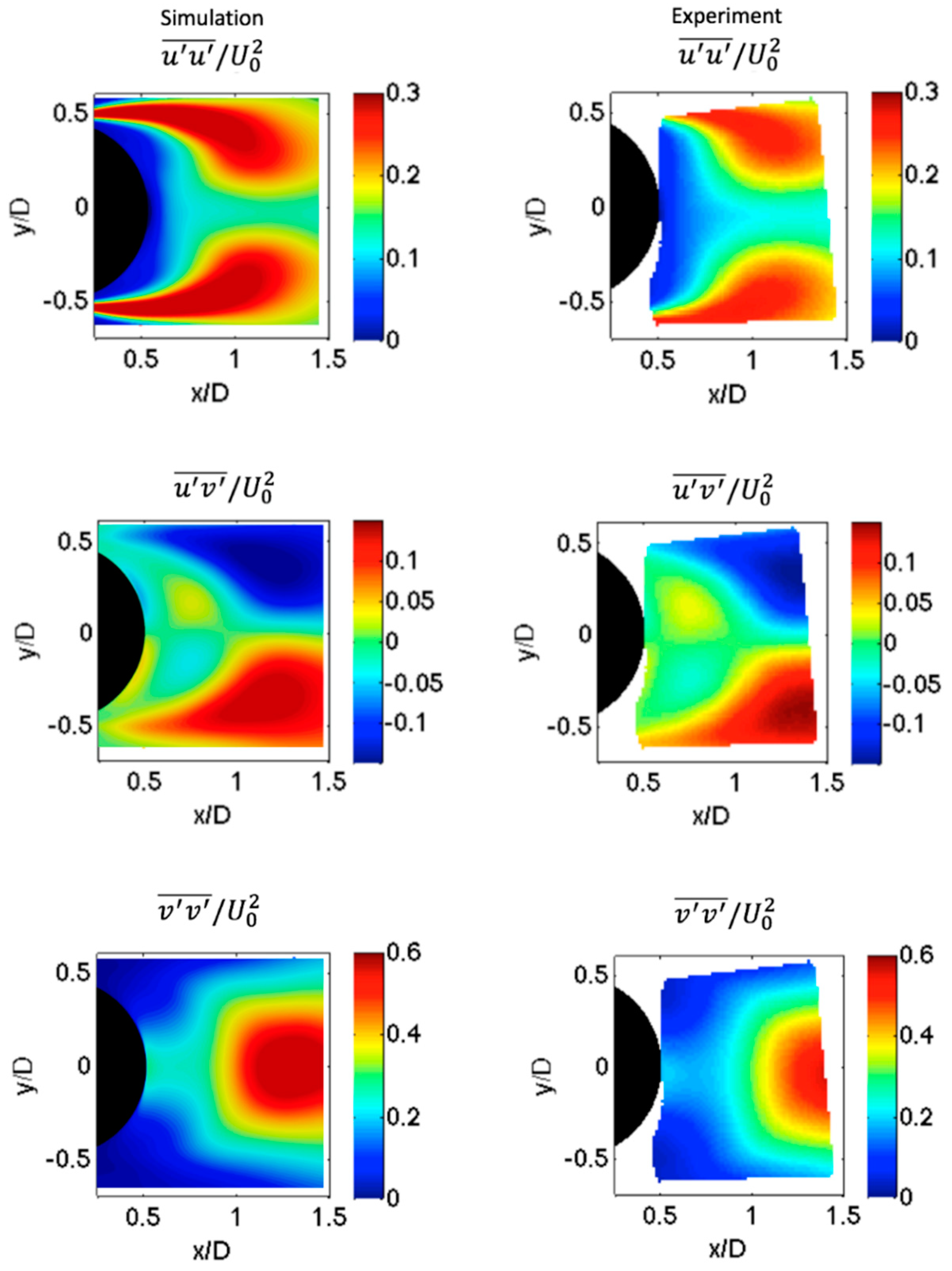
Reynolds stress distributions from simulations and experiments are presented in
Figure 14. The streamwise normal component
peaks at approximately
downstream in both experiments and simulation results. The vertical normal stress
reaches a maximum at
and
in the simulation and experiment, respectively, which indicates that the shed vortex detaches from the cylinder slightly further downstream in the experiments. The distribution of the shear stress component
gives average length of eddy formation.
Similar to , the streamwise location of its peak from simulation is located upstream of experimental data. Generally, the contours indicate that the simulation predicts peak turbulence levels that are located slightly nearer the cylinder than the experiment indicates, with maximum and minimum values similar across the experiments and simulations.
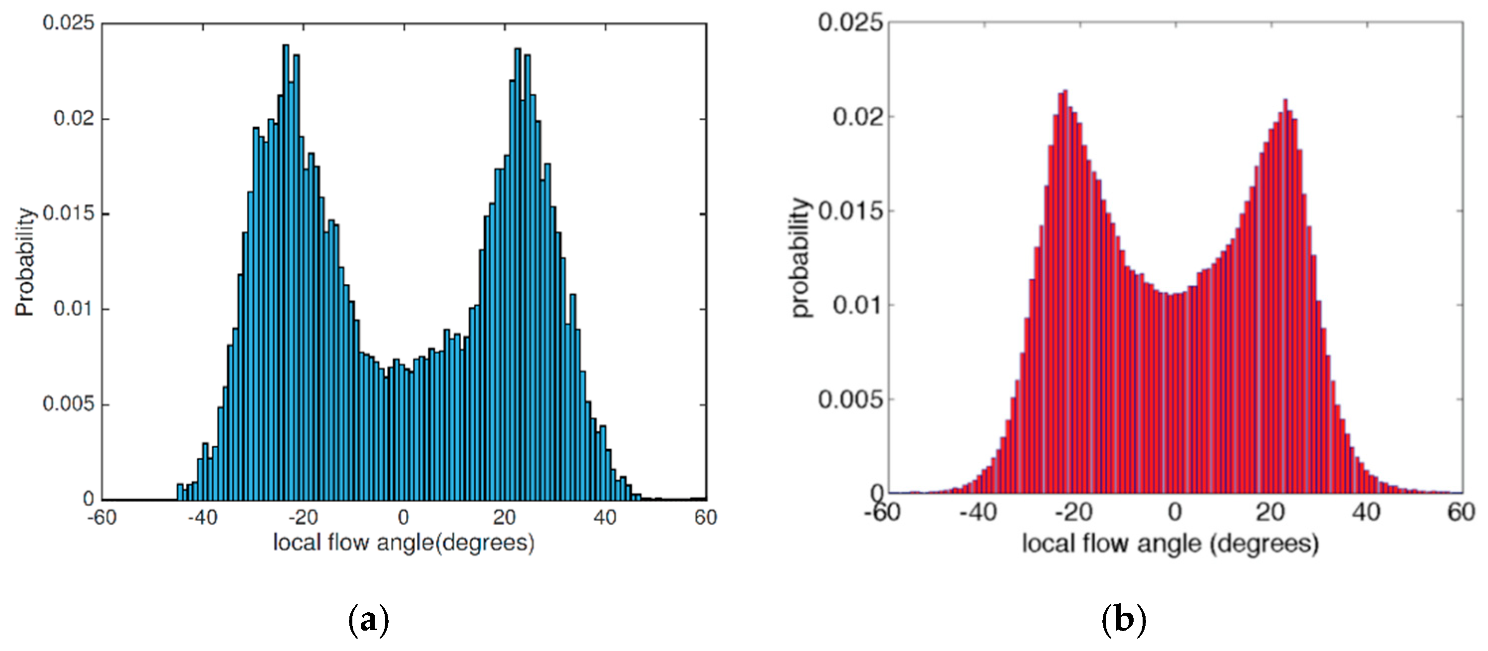
The local flow fluctuations in cylinder wake determines the boundary layer dynamics on the downstream objects. Instantaneous velocity components are sampled at frequency and the flow angle is calculated at four locations downstream of the cylinder center: , , and .
The diffusion and break down of turbulence structures lead to more evenly local flow angles distribution. At
downstream, where the airfoil sits in the surrogate model, the distribution peaks at
with extreme values up to
(
Figure 15). Flow angle at airfoil position is also extracted from PIV data, compared with simulation data at
, both peak at
with probability density value around 0.23. The experiment shows slightly shallower trough, which indicates more low amplitude fluctuations that are not captured in simulations.
5. Unsteady Boundary Layer on Airfoil
The cylinder flow analysis presented in the last section demonstrated the ability of the Langtry-Menter transition model implemented in a DDES formulation in predicting unsteady flow features. This section presents the unsteady flow dynamics on the downstream airfoil, the features of high blade loading fluctuations due to unsteadiness and transitional boundary layers are of interest in the fluid dynamics of full-scale wind turbine blades, making the surrogate problem a comprehensive test case for model development and validation. Along with the cylinder-airfoil setup case, the same airfoil in clean flow is also tested. The only difference is the removal of the upstream cylinder (9 million total cells).
5.1. Instantaneous Flow Field
Due to the periodic nature of the cylinder wake, the boundary layer response on the airfoil also shows periodic dynamics. The periods of the boundary layer dynamics is obtained from the lift and drag forces action on the airfoil, several other flow fields are analyzed at multiple phases within one cycle. With the presence of downstream airfoil, the cylinder shedding frequency increases from to , the existence of downstream airfoil alters the vortex shedding by Our wind tunnel experiments did not test the cylinder flow in the full-model setup.
The mean and RMS of
and
for both cases and XFOIL result are summarized in
Table 4. Airfoil in clean flow has much smaller fluctuations in the force coefficient, mean value matches the RMS value. In contrast, airfoil in cylinder flow experiences significant oscillations, the RMS values of both lift and drag are significantly higher than the corresponding mean value.
The spectral analysis shows the lift fluctuation coincides with the cylinder vortex shedding at and the drag force fluctuation is exactly twice the rate of the lift force. We conclude that the periodic vortex shed from cylinder is the main driver of the unsteady flow around airfoil.
The blending function
is used to regulate TKE destruction as mentioned in last section. Inside the boundary layer, where the specific dissipation
is high,
remains value of 1 and the original RANS formulation is preserved (see an example distribution in
Figure 16). Outside the boundary layer
in the region of fine mesh (i.e., small
) and high TKE (inside eddies).
From
Figure 16, the distribution of
is concentrated around the cylinder and airfoil where the mesh is refined for transition prediction. As the grid size increases from cylinder surface to
downstream of the rear stagnation point,
decreases to
in the outer regions of the eddies, which indicates extra
modeled TKE is destructed compared with RANS model. In the core of the eddies, where local TKE is high,
remains
. As the vortex interacts with the airfoil, where mesh is refined again, the eddies are stretched around the leading edge and
resumes to the same level as in the cylinder near wake.
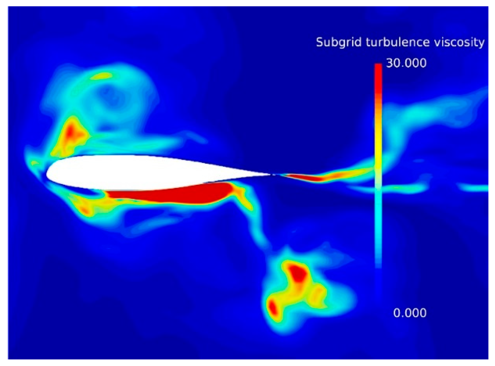
Figure 17 is the instantaneous eddy viscosity distribution around airfoil in the cylinder wake. The alternating vortex structures exist on either side of the airfoil, notice there is a shear layer leaving the airfoil trailing edge which interacts with the cylinder vortices.
There is a strong correlation between and outside the boundary layer. reaches maximum in the center of the vortices and the eddy viscosity, which is proportional to TKE, is attenuated (e.g., see suction side near the leading edge). The rotational flow interacts with the airfoil boundary layer and cause local increase in TKE and eddy viscosity, the blending function follows the same trend. By the time the eddy reaches trailing edge, the attenuation effect of decreases the eddy viscosity significantly.
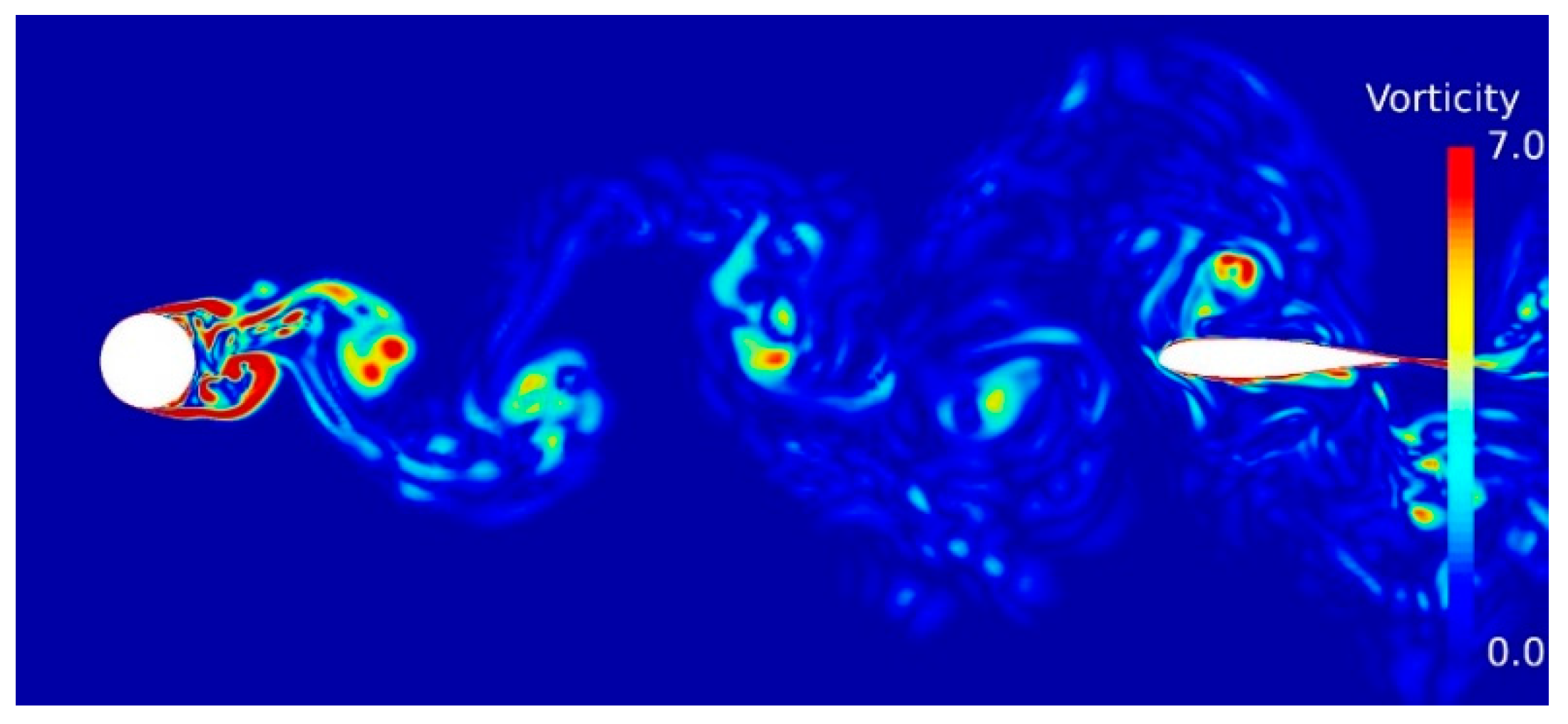
Inspecting the fluid force acting on the airfoil, we found the cylinder vortices are the main driver of the airfoil unsteadiness. The normalized vorticity field
is concentrated inside the Karman vortex and the width of the wake grows as the they travel downstream as shown in
Figure 18, the coherent turbulence structures break up and stretched as they interact with the airfoil boundary layer (
Figure 19).
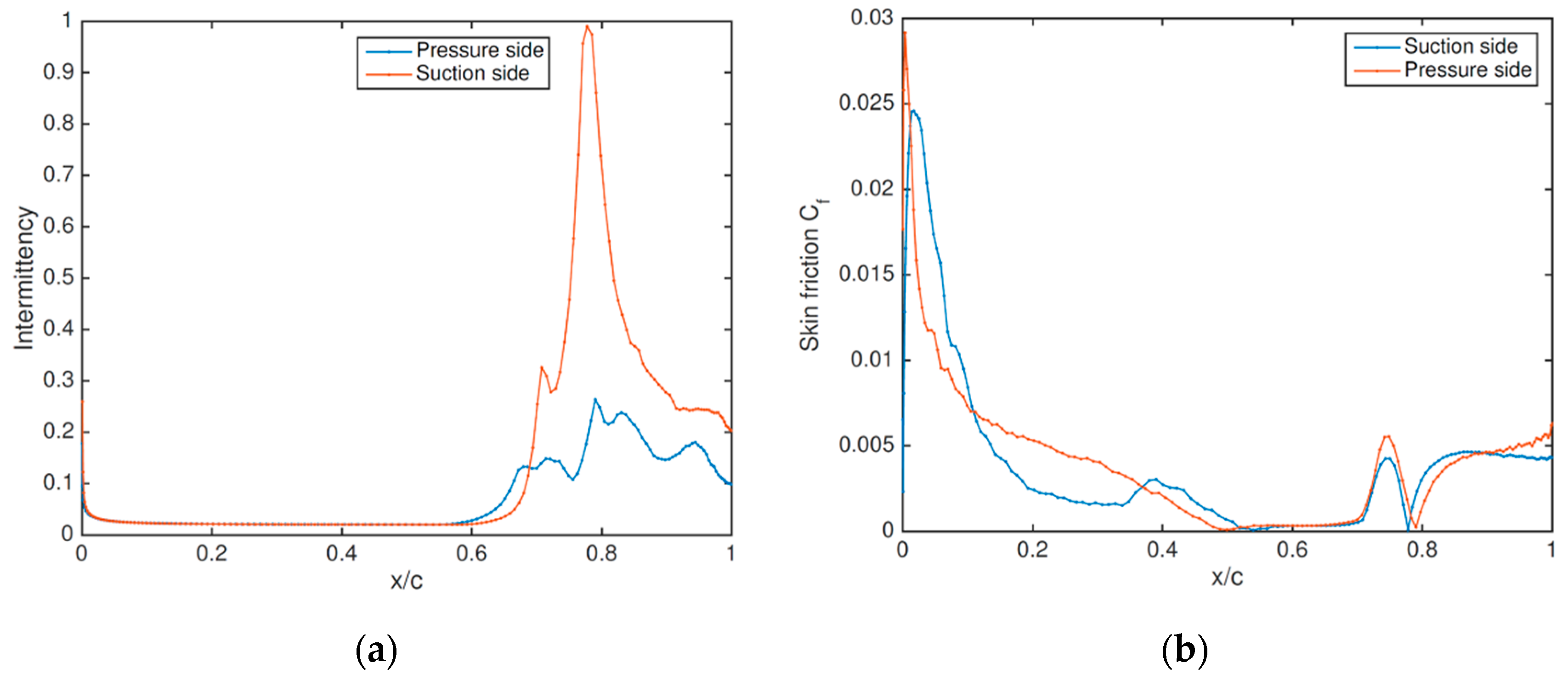
The LM turbulent intermittency field gives a clear indication of laminar boundary layer separation, the airfoil boundary layer in clean flow remains laminar before separating and the transition location after separation is clearly visible from LM intermittency distribution on airfoil surface as shown in
Figure 20a. Boundary layer transition initiates on both sides at approximately
, which is confirmed by the skin friction distribution (
Figure 20b). The separation bubble extends
downstream of the transition point and the boundary layer flow reattaches at
on both sides.
Airfoil boundary layer inside cylinder wake is fully turbulent and attached at all time. The surface LM intermittency remains low ( over of the airfoil surface), which indicates the existence of laminar viscous sublayer in the attached boundary layer. Experiments looked at boundary layer parameters from to at interval and found it remained attached and turbulent at all locations, which confirms our observation from simulation.
To demonstrate the variations of the velocity magnitude inside boundary layer, the instantaneous velocity component that is parallel to the airfoil surface at
,
and
within one cycle are plotted in
Figure 21. The instantaneous profile is averaged within 8 phase bins using phase averaging based upon the shedding phase of the cylinder vortex. No reverse flow is observed in the vicinity of the wall at the all positions, therefore there is no boundary layer separation at all time. Compare velocity profile at
with
, it is noticeable that the boundary layer has thickened as flow travels downstream. There is phase lag across three locations, which will be inspected further in phase-averaged profiles.
5.2. Mean Flow Field and Flow Statistics
5.2.1. Mean Pressure and Velocity Field
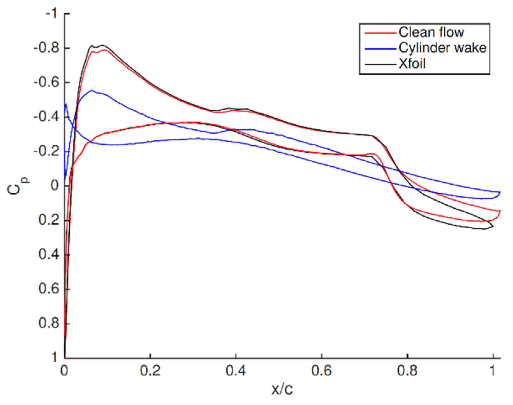
Figure 22 is the predictions of mean pressure distribution from simulation results of airfoil in clean flow and cylinder wake. The pressure distribution in clean flow agrees with XFOIL data from leading edge to the reattachment locations. The CFD data predicts lower pressure gradient than XFOIL data in the turbulent boundary layer after reattachment.
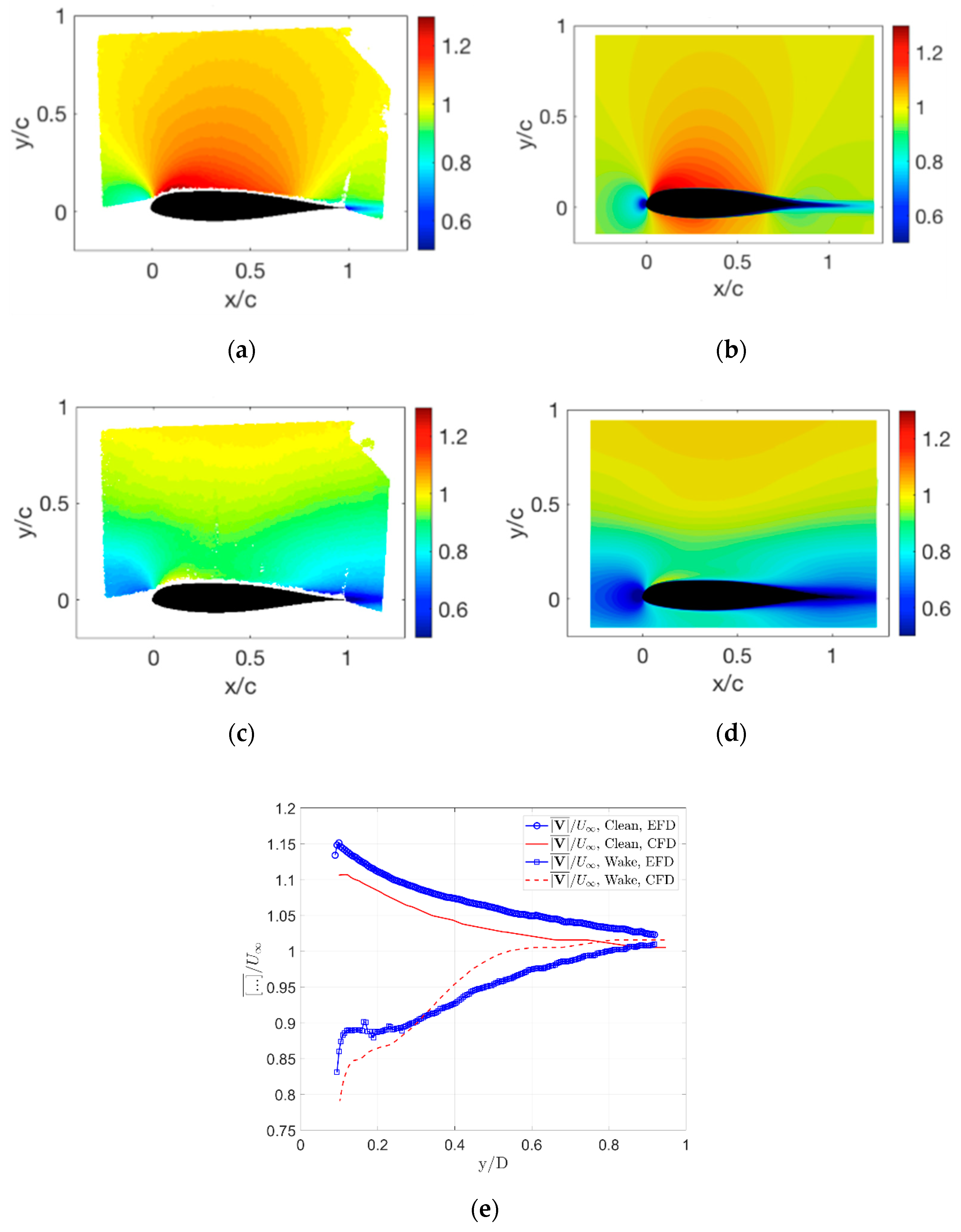
Mean flow velocity around the airfoil in clean flow and cylinder wake is extracted from both experimental and simulation data (
Figure 23). Note that the PIV data are only available on the suction side of the airfoil due to limitations of the optical arrangement. Flow reattaches on both sides of the airfoil in clean flow at
which is marked by the sudden change in mean velocity field (
Figure 23a,b). Comparing the EFD and CFD results for the clean flow, the pressure gradient induced by the airfoil appears to have a slightly different far-field behavior; however, based upon the comparison of
Figure 23e at
= 0.5, small differences between the experimental and computation boundary conditions are likely to drive this difference: the discrepancy between results is nearly constant at all distances from the airfoil.
The presence and influence of the mean wake flow is clearly evident in the case of the airfoil in the cylinder wake (
Figure 23c,d). A comparison between the EFD and CFD results at
= 0.5 (
Figure 23e) lead to some notable observations. In contrast to the clean flow case, even the boundary layer is highly pronounced and of a scale comparable to the large-scale mean flow gradients. Both the experiment and simulation show a similar thickness for the boundary layer this station. As is evident in the contours, but highlighted by the line plots, the mean flow due to the circular cylinder wake has some notable differences between the experiment and simulation. The gradient of the wake is greater for the CFD results, indicating that turbulent diffusion in the experiment was greater. The question of small differences in boundary conditions must be reconsidered in the assessment of these differences. Further, the small differences in the near-cylinder turbulence seen in
Figure 14 will result in changes in the evolution of the turbulent wake development over the 10.67 diameters of spacing between the cylinder and airfoil. These results, while encouraging for the application of transition models in the DDES framework, highlight the challenges involved with providing experimental boundary conditions of sufficient fidelity for high confidence turbulence model assessment and improvement.
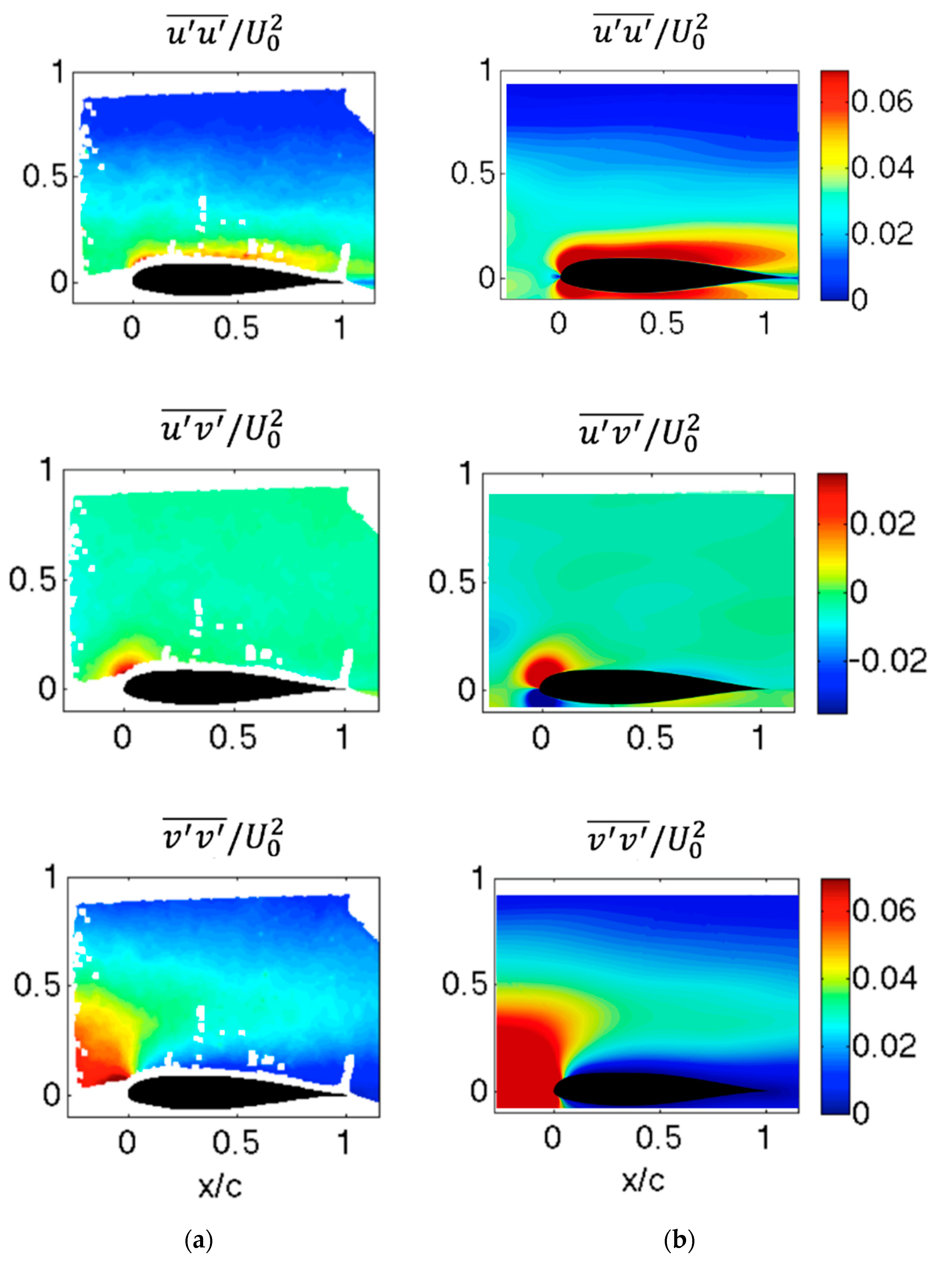
5.2.2. Reynolds Stress
Figure 24 is a comparison of three normalized Reynolds stress components around airfoil in cylinder wake. The experimental data is only available on the suction side and the PIV system resolution limited the measurement to the outer region of boundary layer.
The magnitude and distribution of all three Reynolds stress components from simulation agree with experimental data, however the experimental results contain more stochastic structures from the decay of cylinder wake eddies. The shear stress term peaks at leading edge due to high distortion of turbulence structures in cylinder wake, same feature is absent in the case of clean inflow.
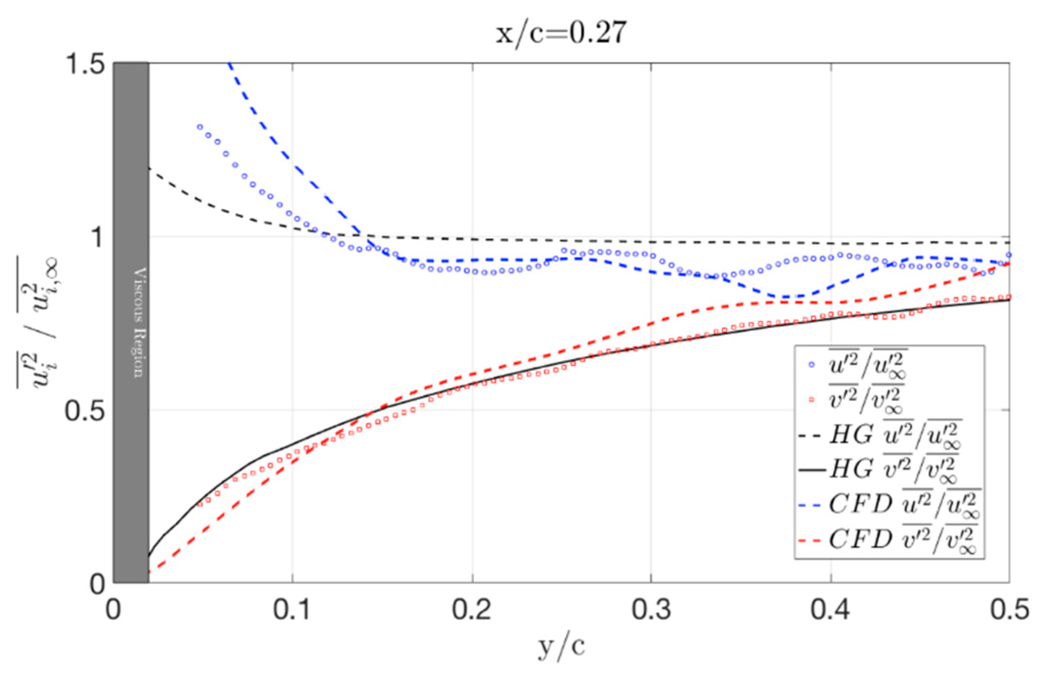
The most noticeable feature of Reynolds stress field is the redistribution of fluctuation energy between the normal stress components. The streamwise component
increases significantly from the leading edge while the transverse component
reduces at the similar rate. The redistribution of the normal stress as approaching the solid surface is an invisicid effect described by rapid distortion theory (RDT,
Figure 25). The Hunt and Graham (HG)’s results for an instantaneously appearing flat-plate [
34] are rescaled with
and
to fit the measured data in experiments and simulations. The experimental and simulation results that are represented by dot and dash lines follow the same trends as the theoretical prediction with slightly higher gradient in
close to the wall. According to Pope [
35], the Reynolds stress component is proportional to the correspond strain rate and the pressure fluctuation
, as the strain rate component in transverse direction reduces on airfoil surface, the transverse normal stress
is redistributed to the streamwise and spanwise components. The redistribution features are absent from the clean flow case since the pressure fluctuation
must present to initiate the mechanism [
17]. The redistribution of Reynolds stress also has significant effects on turbulence energy of the streamwise and transverse velocity components
and
.
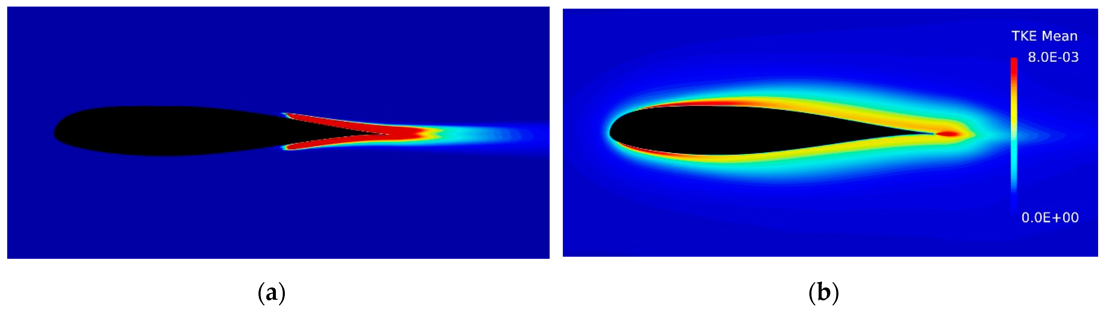
5.2.3. Mean Turbulence Kinetic Energy
The mean grid-resolved TKE around airfoil which sits in clean inflow and cylinder wake are shown in
Figure 26, in both cases the TKE field is normalized by
. TKE starts to grow downstream of the laminar separation point on the airfoil in the clean flow case, the distribution is concentrated inside the separated boundary layer, which confirms that RANS model is preserved.
For the airfoil in cylinder wake, TKE is concentrated in the thin boundary layer at leading edge and it diffuses outwards as traveling downstream. The peak at the trailing edge is due to the free shear layer leaves the airfoil.
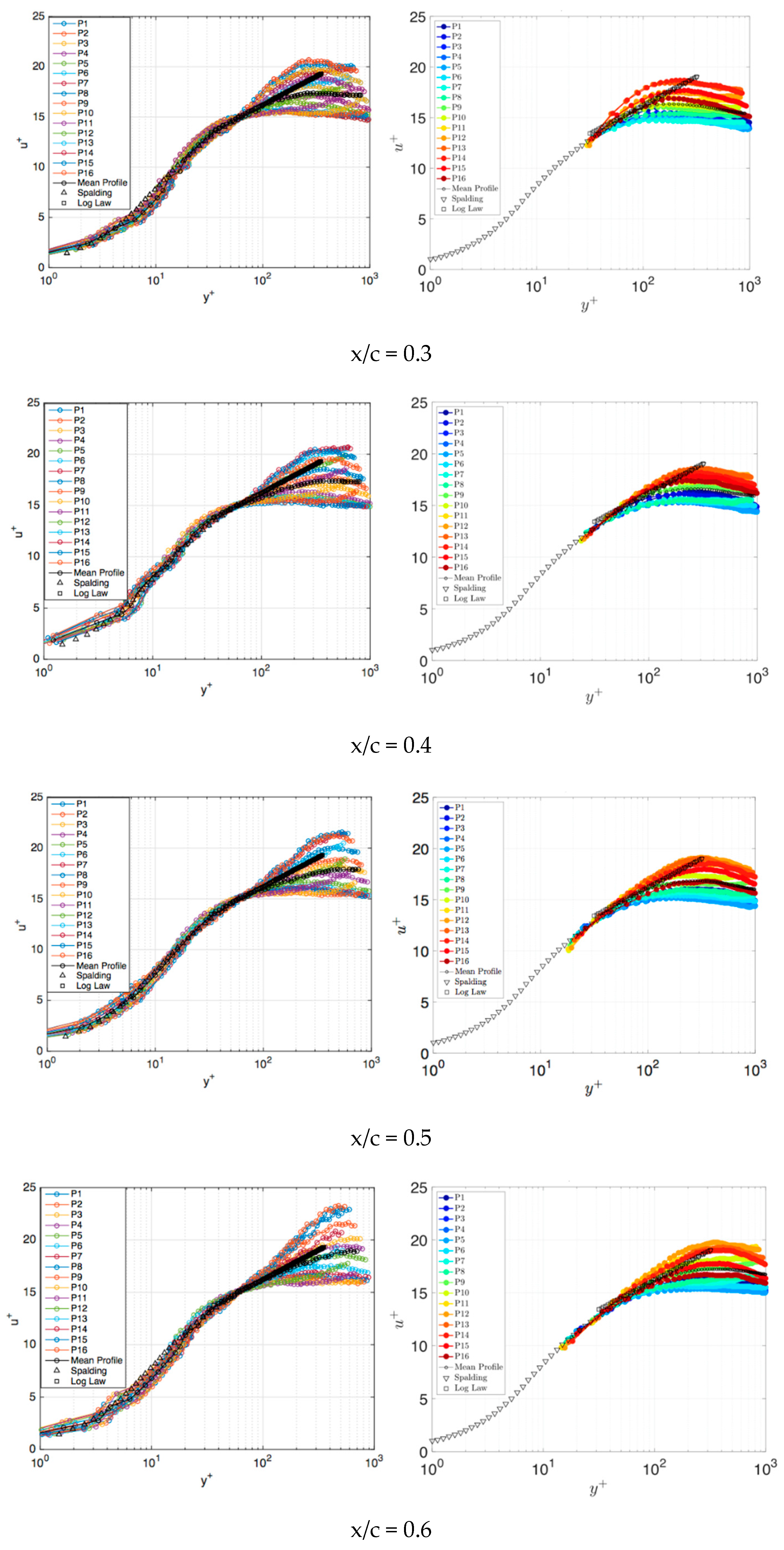
5.2.4. Phase-Averaged Boundary Layer Profiles
Probes are placed from airfoil surface up to
in the wall-normal direction. The phase of a band limited signal
is determined by Hilbert transform [
36]
:
The phase is calculated as:
The simulation data contains over 140 periods of the oscillatory flow around the airfoil, each cycle is subdivided into 16 phases with a width of
phase angles. The velocity profile is then averaged within each phase of all cycles. In order to plot the profile in terms of non-dimensional parameters
and
, least square method is adopted to find the value of friction velocity
that best fit the profile in viscous sublayer (
) and log layer (
).
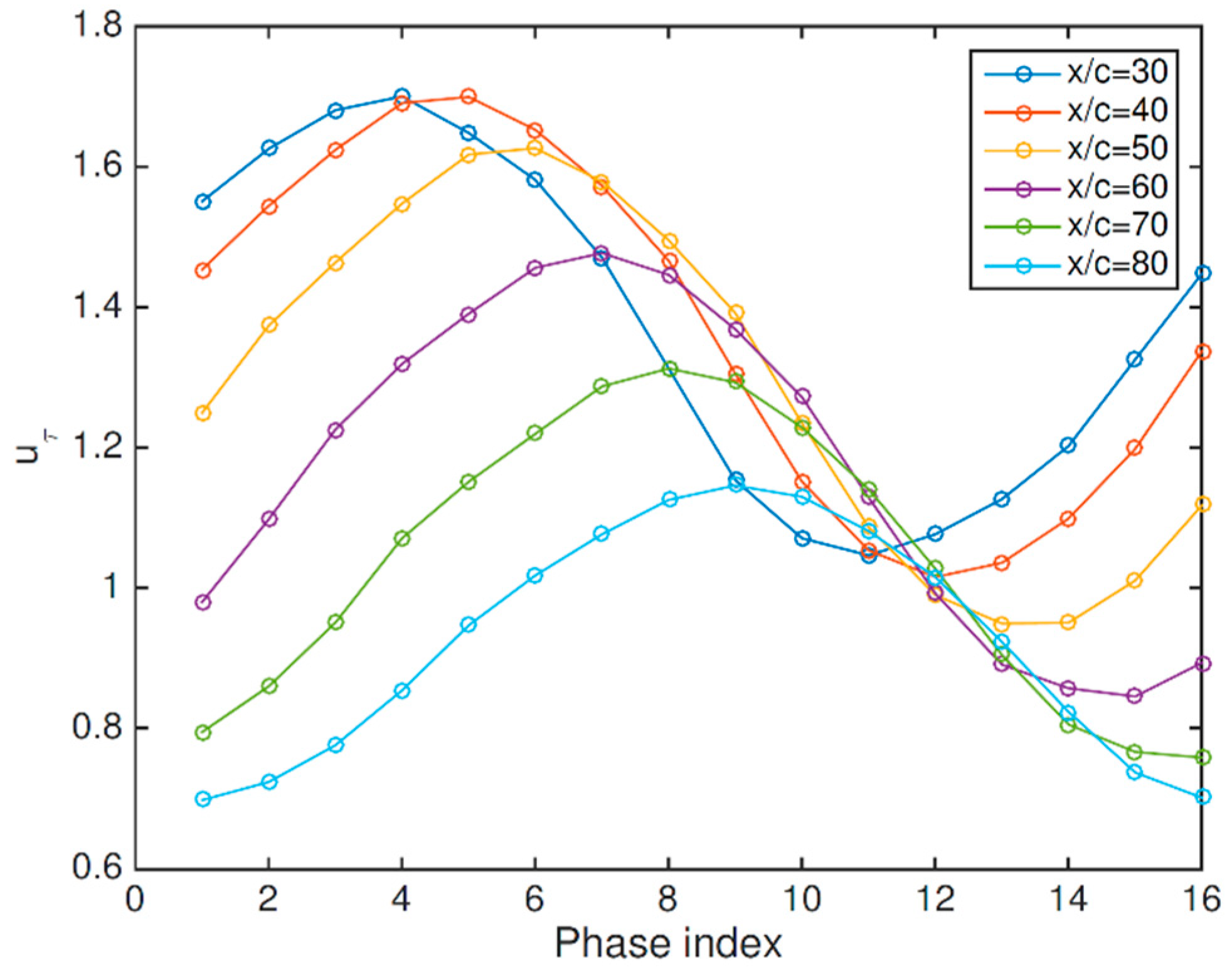
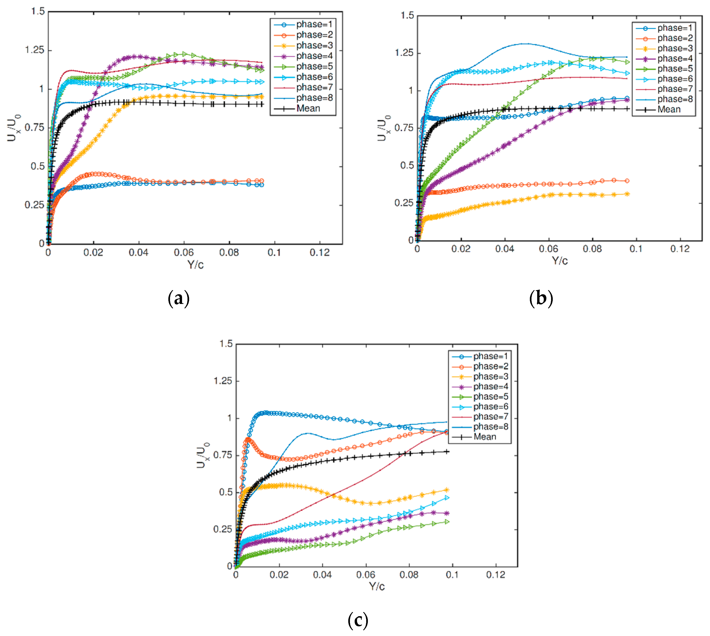
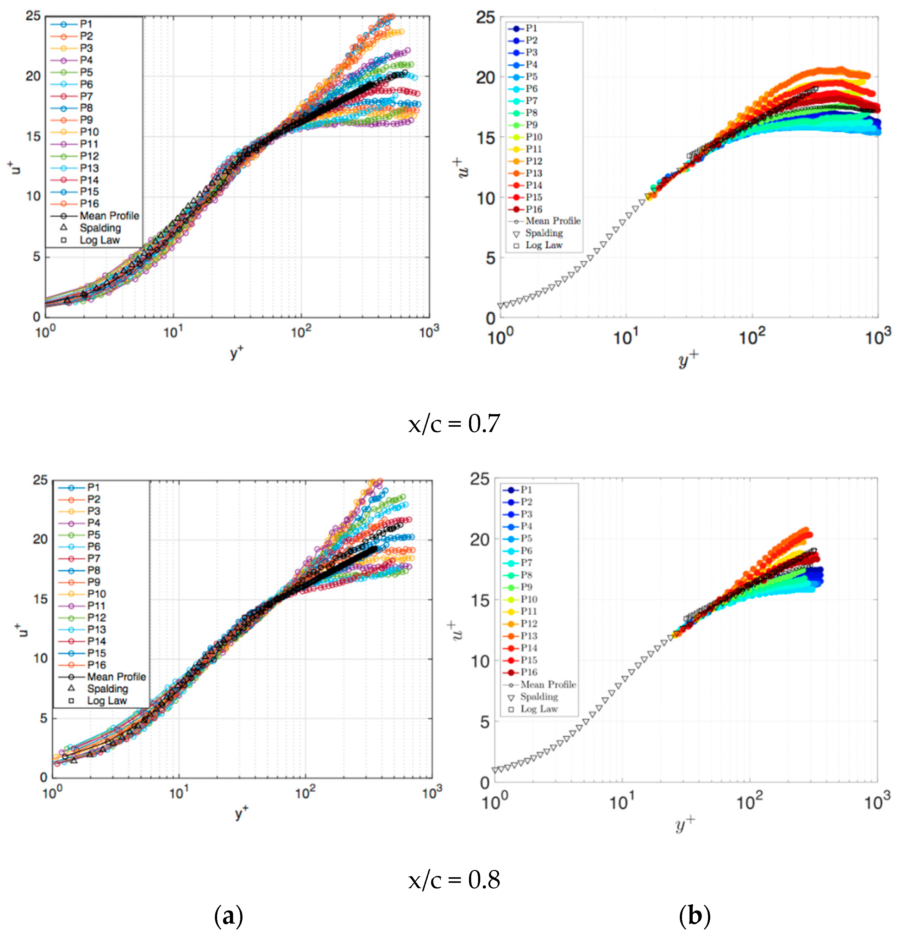
Figure 27 is a plot of the friction velocity distribution for each phase at every chordwise positions. There is a consistent phase-shift and decrease in
as moving downstream, from the amount of phase-shift from station
to
together with the flow period, the wave speed is
.
Phase-averaged boundary layer profiles from simulation and experiments are plotted in
Figure 28 together with the Spalding’s single formula for the “Law of the Wall” [
37], viz.:
which is valid through the viscous sublayer and the log layer.
The Log Law curve follows the standard “Law of the Wall” formulation:
The experimental data is available from due to the limited PIV system resolution near surface. Two formulations of “Law of the Wall” converge from approximately and the mean velocity profile is also plotted on the same figure.
There are several notable observations: although the least square method that fits the curves takes the data between and into account, every curve at each chordwise position converges at approximately and diverges above it, which indicates the cylinder wake dynamics dominate the wake region above . The simulation data shows the magnitude of the oscillation in the wake region gradually grows in chordwise progression, while the experimental data predicted nearly constant variations ) of the boundary layer profile at . The flow in the boundary layer wake region carries more energy in the simulation results.
Even in the highly-unsteady cylinder wake, the Law of the Wall is still valid in the low-momentum viscous inner regions, which confirms the validity of its adoption in many wall-modeled RANS and LES applications. Finally, the Law of the Wall agrees better with the phase and mean profiles of downstream locations, where the boundary layers are significantly thicker.
6. Conclusions and Future Work
The main objective of this study is to find an improved turbulence modeling approach that can capture the flow physics presented in the boundary layer of a wind turbine blade inside the atmospheric boundary layer and upstream turbine wake. A surrogate model was designed to keep the computational and experimental costs manageable while preserving the key flow physics present in the full-scale problem. We realized the LES-type turbulence model is beyond the computing power available currently even just for the surrogate model, while also noting promise from previous studies that show the value of using turbulence models that include boundary layer transition formulation into the RANS model for improved blade aerodynamics predictions.
The delayed detached eddy simulation (DDES) was chosen as the hybrid modeling methodology for its superior performance over RANS in massively-separated flow regions at affordable computational cost. The implementation of the transition model was verified against the simulation data by its original authors and validated using well-established experimental data. The integrated hybrid transition turbulence model was then applied to the circular cylinder at subcritical Reynolds number. Compared with the complementary experimental data, the mean flow dynamics, vortex shedding frequency and Reynolds stresses in the cylinder near wake were well captured by transition hybrid model.
Applying the transition hybrid model to the full-model led to some major discoveries in unsteady flow physics. The passage of the eddies dominates the pressure variations on the airfoil. Despite large local flow angle variations, there was no separation on the airfoil in the cylinder wake. Examining the Reynolds stress distribution, we found redistribution of the normal stress components, which is an inviscid effect predicted by rapid distortion theory. Inspecting the blending function distribution, the hybrid model operated in RANS mode inside the cylinder and airfoil boundary layer, where the local mesh resolution cannot afford resolving turbulence structure. The phase-averaged boundary layer profiles on airfoil followed the law-of-the-wall in the inner region.
The major downside of our current surrogate model is the scale mismatch compared with the full-scale problem as summarized in
Table 1, and the authors have interest in addressing this through future work. The inflow unsteadiness is the key parameter in determining the blade dynamics, other than the blade root, and the reduced frequency of the full-scale blade is approximately one or two orders of magnitude lower than our model. By manipulating the definition of Strouhal number
and reduced frequency
we have
,
maintains
for
, such that the reduced frequency
is determined by the ratio of the chord length to the cylinder diameter—a scale-up model design will focus on increasing the cylinder size. Another benefit of the larger cylinder is increasing the turbulence length scale that can engulf the whole airfoil as the atmospheric turbulence does to the full-scale turbine blade. The flow field containing the larger diameter cylinder would contain key physics similar to the harmonic gust problem described by the Sears function.
In conclusion, the transition hybrid RANS/LES model showed its potential in calculating unsteady flow physics of a model wind turbine blade. Compared with RANS model, it resolves the turbulence structures down to the local grid size, which are averaged and smeared in unsteady RANS simulations; compared with LES models, the computational cost is affordable for most practical problems, and the meshing process is less stringent since the new model can, at worst, operate in RANS mode. The integration of the transition model enabled the accurate prediction of laminar separation, transition and flow reattachment, which were proven to be first-order factors in calculating blade aerodynamics.


