1. Introduction
In material processing, such as semiconductor crystal growth or continuous casting of steel, applying a magnetic field is the most promising method to control molten metal flows. Among various types of magnetic field, the stationary magnetic field is used to damp out electrically conducting melt flow whereas the rotating magnetic field is considered to be useful to stir the melt flow due to the Lorentz force. The rotating magnetic field is a type of alternating magnetic field and its strength, field shape and angular frequency are the crucial parameters. Since there is a variety of rotating magnetic fields, the effect on the conducting melt flow also varied widely.
As a pioneering work, Moffat [
1] investigated the effect of a rotating magnetic field on the electrically conducting fluid flow in a cylindrical vessel. He pointed out that the field strength and angular frequency are the two most important factors on the condition that the skin effect takes place. Richardson [
2] analytically demonstrated the critical condition of the onset of secondary flow for an electrically conducting fluid in an infinitely long cylindrical enclosure. His analysis is limited to the case that the applied rotating magnetic field is weak enough to define the magnetic Taylor number and its angular frequency is slow enough to neglect the skin effect. Sneyd [
3], Davidson and Hunt [
4], and Davidson [
5] also performed fundamental studies on the flow driven by a rotating magnetic field. In references [
2,
3,
4,
5], the common feature of the treatment of analysis is to neglect the skin effect and to use the time-averaged Lorentz force as a driving force in the azimuthal direction.
Concerning the application of the rotating magnetic field on the crystal growth, not only the fluid flow but also the temperature field and/or concentration field should be taken into account. Such studies can be found in references Barz et al. [
6], Ghaddar et al. [
7], Mößner and Gerbeth [
8], Ben Hadid et al. [
9], and Patzold et al. [
10] and some of these include the discussion of the flow transition. Friedrich et al. [
11] studied the effect of a rotating magnetic field on the Rayleigh-Bénard convection by using the magnetic Taylor number. Vizman et al. [
12] demonstrated the three-dimensional simulation for a flow driven by a rotating magnetic field under the influence of buoyancy caused by the temperature difference. Volz and Mazuruk [
13,
14] investigated the influence of a high-frequency rotating magnetic field on the flow instability within a cylindrical enclosure heated from below with considering the skin effect. Grants and Gerbeth [
15,
16] conducted stability analyses for both axisymmetric and three-dimensional flows driven by a rotating magnetic field in a cylindrical enclosure. Later, they also experimentally investigated the flow transition to turbulence [
17].
The group of Martin and Witkowski studied the flow driven by an arbitrary frequency of the rotating magnetic field [
18], and an asymmetric flow driven by a low frequency of the rotating magnetic field [
19]. They also studied that a case of high frequency for a finite length of cylindrical enclosure [
20], the influence of the rotating magnetic field on the instability of the thermo-capillary convection for the floating zone method [
21], and the effect of a rotating magnetic field on a flow in a rotating cylindrical vessel [
22]. Feonychev and Bodareva [
23] considered the effect of a rotating magnetic field on the flow stability subjected to the gravitational force and/or surface tension. Nikrityuk et al. [
24] carried out numerical computation for a flow driven by a rotating magnetic field in a cylindrical enclosure with various aspect ratios. Lyubimov et al. [
25] performed linear stability analysis for a flow driven by a rotating magnetic field in a cylindrical enclosure whose axis is set horizontally and the temperature gradient is parallel to its axis.
The group of Ando and Ueno [
26,
27,
28,
29,
30] studied the induction pump for a liquid metal using the rotating and twisted magnetic field experimentally, numerically and theoretically. The rotating twisted magnetic field, which can drive the molten liquid both in the azimuthal and axial directions, is generated by a stator with three pairs of helical windings. They carried out a molten metal circulation experiment using molten gallium and confirmed that the conventional slip-thrust relation is satisfied in the experiments [
26,
27,
28]. Numerical simulation with the same condition performed in a previous experiment was carried out under the magnetic Stokes approximation for a small shielding parameter [
29]. Asymptotic analysis [
30] for a small magnetic Reynolds number clarifies that the temporal mean value of the axial driving force is almost uniform but rather small when the twist ratio is considerably smaller than 1.
As mentioned above, the use of a rotating magnetic field is rather limited to the metal processes such as the control of the semiconductor melt and/or stirring and driving of the electrically conducting fluids. The most important point in such numerical analyses related to the rotating magnetic field is to model the Lorentz force which is responsible for the liquid metal flow. Most of the literature mentioned above assumed axisymmetric flow, neglecting the skin effect, low magnetic field, and time-averaged Lorentz force. In such a situation, the magnetic Taylor number is the only significant parameter that governs the fluid flow. However, recent development of superconducting magnets enables us to utilize a high magnetic field. Therefore, we aim to elucidate the fundamental mechanism of the flow instability caused by the strong rotating magnetic field in which the electric potential cannot be neglected. The present paper describes the modeling of the Lorentz force in which the influence of the number of pole-pairs is taken into account and carries out linear stability analysis of liquid metal driven by a multi-pole rotating magnetic field.
2. Configuration of Problem and Governing Equations
2.1. Problem Considered
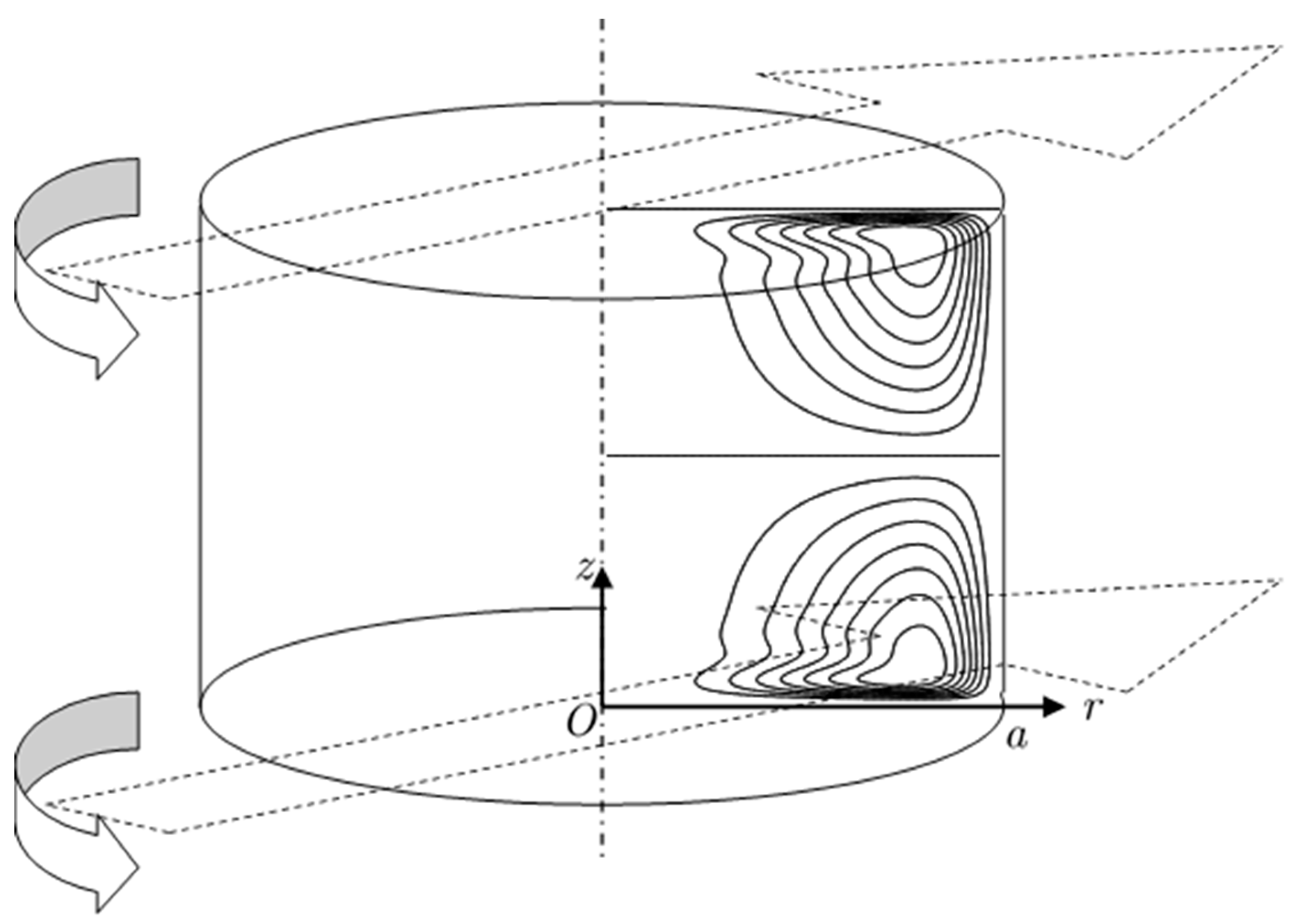
As shown in
Figure 1, we consider a fundamental case that an electric conducting fluid filled in a cylindrical vessel is subject to an applied rotating magnetic field. The rotating magnetic field induces the electrical current density in the conducting fluid and it interacts with the magnetic field to generate the electromagnetic force. This phenomenon seems to be easily understood but it widely depends on both the angular velocity and the strength of the rotating magnetic field. We consider that the cylindrical vessel is stationary and, therefore, the boundary layer tends to become unstable due to the Taylor-Görlter instability in the vicinity of the side wall. The electrically conducting fluid considered is assumed to be an incompressible Newtonian fluid and the viscous dissipation and Joule heating are neglected in this analysis. The continuity and momentum equations are as follows:
The external force in the momentum equation is related to the electromagnetic fields, which are governed by the electromagnetic equations as follows:
Equation (3) is the Faraday’s law, Equation (4) is the Gauss’s law for magnetism, Equation (5) is the Ampère’s law, Equation (6) is the Ohm’s law, Equation (7) is the conservation of electric charge, and Equation (8) is the electromagnetic force. In order to satisfy Equation (4), a vector potential is introduced, as shown in Equation (9), together with the Coulomb gauge of Equation (10).
From Equation (3), the electric field can be expressed with both the vector potential and scalar potential, as shown in Equation (11).
2.2. Formulation of Rotating Magnetic Field in Non-Conducting Media
In this section, the formulation of a multi-pole rotating magnetic field in non-conducting media is considered. The rotating magnetic field satisfies both curl-free and divergence-free conditions at the place where the electric current density does not exist in non-conducting media. One of the possible vector potentials, which satisfies the Coulomb gauge, is expressed with a harmonic function.
In the polar coordinate system, a vector potential having only the axial component is considered herein.
We assume that the axial component of the vector potential can be divided into the amplitude function and the wave function rotating in the azimuthal direction as follows:
where,
m is the number of pole-pairs,
ω is the angular frequency of the applied rotating magnetic field, and
Ω is the angular velocity of the field. Equation (14) is substituted into Equation (13), and subsequently, we can obtain the Laplace equation regarding to the amplitude function.
Since we assume that the boundary condition for the magnetic field at the cylinder wall (
r =
a) is
B0, the amplitude function of the vector potential is derived as follows:
We obtain the axial component of vector potential.
The radial and azimuthal components of the magnetic field can be derived.
It is easily understood that these two equations satisfy the Laplace equations for the applied magnetic field as follows:
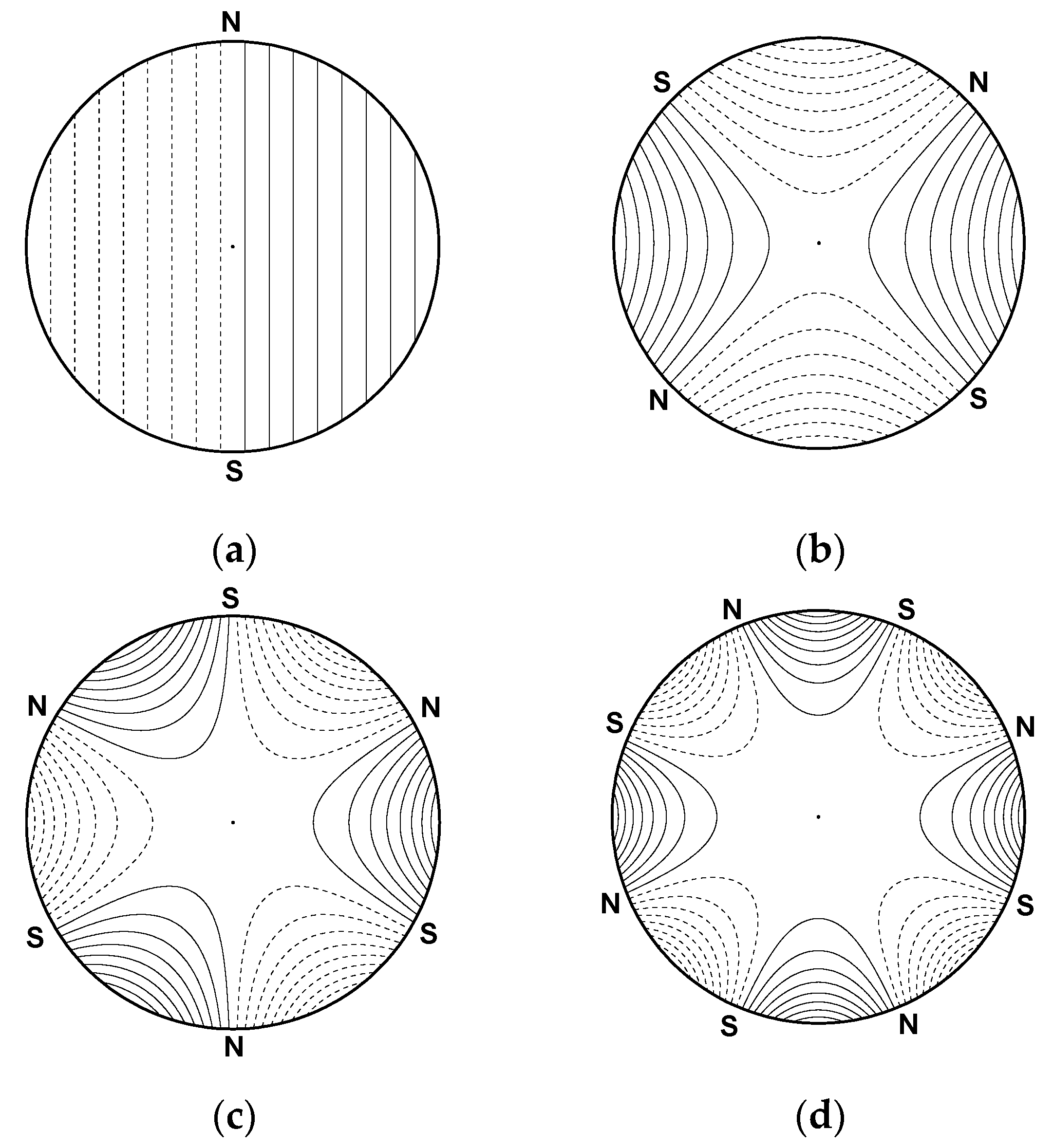
Figure 2 shows the magnetic field lines for several cases of the number of pole-pairs at a time instance. Equation (17) is used for visualization. Where, N and S indicate the magnetic poles. It can be recognized that the magnetic field does not tend to reach the core region as the number of pole-pairs is increased.
2.3. Formulation of Electromagnetic Force
From Equations (5), (6) and (3), the induction equation can be derived.
When this equation is expressed with a non-dimensional form, two non-dimensional numbers appear.
where,
Ω represents the angular velocity of the applied rotating magnetic field,
a is the radius of the cylinder,
νm is the magnetic viscosity,
u0 is the characteristic velocity,
Rω is the shielding parameter, and
Rem is the magnetic Reynolds number. In this paper, it is assumed that the two non-dimensional numbers are much smaller than unity.
Therefore, only the second term on the right-hand-side of Equation (21) is significant and the magnetic field even in the conducting media is assumed to be the same as that in a vacuum. Since the profiles of the vector potential and magnetic field have been obtained as shown in Equations (17) and (18), each component of the electric current density can be calculated using Ohm’s law.
The terms of electric potential have to be obtained so as to satisfy Equation (7) of the conservation of electric charge, and the following Poisson equation is derived.
For the sake of simplicity in computation, we assume that the electric potential has the form as followed by Priede [
31].
Then, we have two Poisson equations, which do not include trigonometric functions.
where, the term of the azimuthal derivative of the axial component of the velocity is neglected in Equation (28) because of the assumption of axisymmetric flow in this study. By solving Equations (28) and (29), the electric potential that appeared in Ohm’s law can be obtained. The electromagnetic force that appeared in Equation (8) is represented as shown in the next equation.
where,
β =
ωt – mθ in Equation (30). As indicated in Equation (30), the electromagnetic force can be divided into the periodic oscillatory part and non-periodic averaged part. In this paper, the double frequency of the wave motion in the electromagnetic force is ignored. The non-periodic averaged force is arranged as follows.
This Lorentz force model derived here is coincident to that developed originally by Priede [
31,
32,
33]. In this paper, the axisymmetric flow driven by the averaged force is considered. By combining Equations (1), (2) and (31), the Navier-Stokes equations, including the electromagnetic force in the cylindrical coordinate, are as follows:
3. Linear Stability Analyses
In this section, electrically conducting fluid flow driven by the multi-pole rotating magnetic fields in an infinitely long cylinder with the radius a is considered.
3.1. Basic Flows
When the influence of the upper and lower ends is neglected, the fluid flow has only the azimuthal velocity and no electric field is generated. Since the inertial term and the electric potential term in Equation (34) disappear, it represents the balance between the electromagnetic and viscous forces.
The solution of the basic flow can be obtained by solving the above equation. After making the equation non-dimensional, we get:
Here, the dimensionless azimuthal velocity, dimensionless radius and the Hartmann number are defined as follows:
The solution to Equation (37) with the no-slip boundary condition at the cylinder wall can be found using the modified Bessel function of the first kind as follows [
34]:
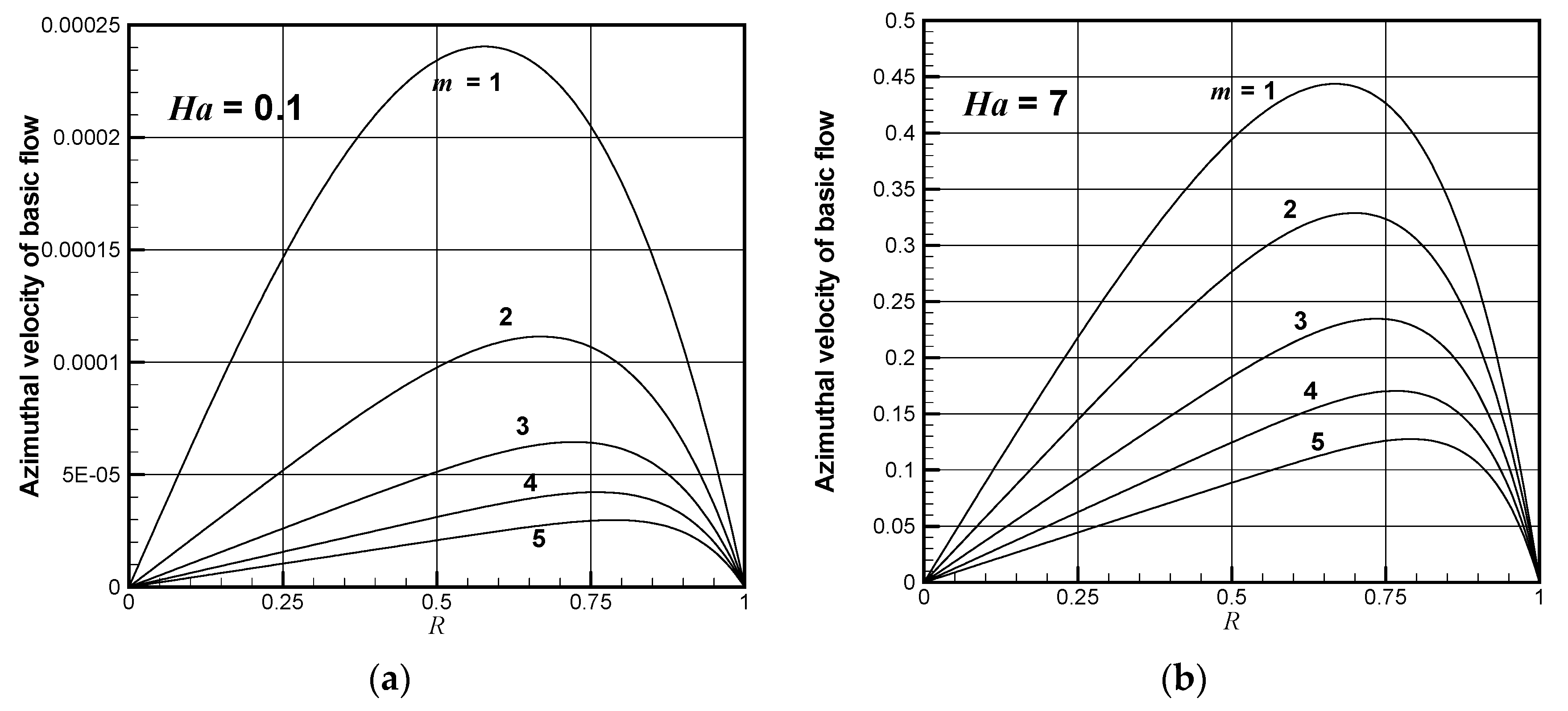
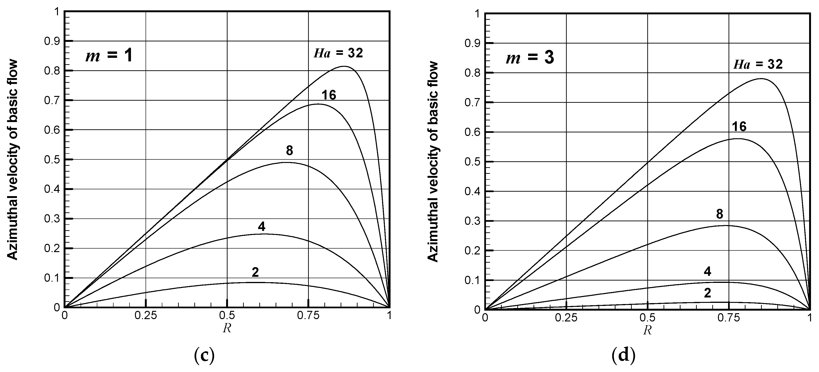
Figure 3 shows the azimuthal velocity of the basic flow for several cases of the number of pole-pairs (
m) and the Hartmann number (
Ha). For a given Hartmann number, the azimuthal velocity decreases as the number of pole-pairs increases. For a given number of pole-pairs, the azimuthal velocity increases as the Hartmann number increases. For an extreme case of
m = 1 and
Ha = 32, the core velocity attains the rigid-body rotation. This means that the core flow rotates with the same angular velocity as that of the applied rotating magnetic field.
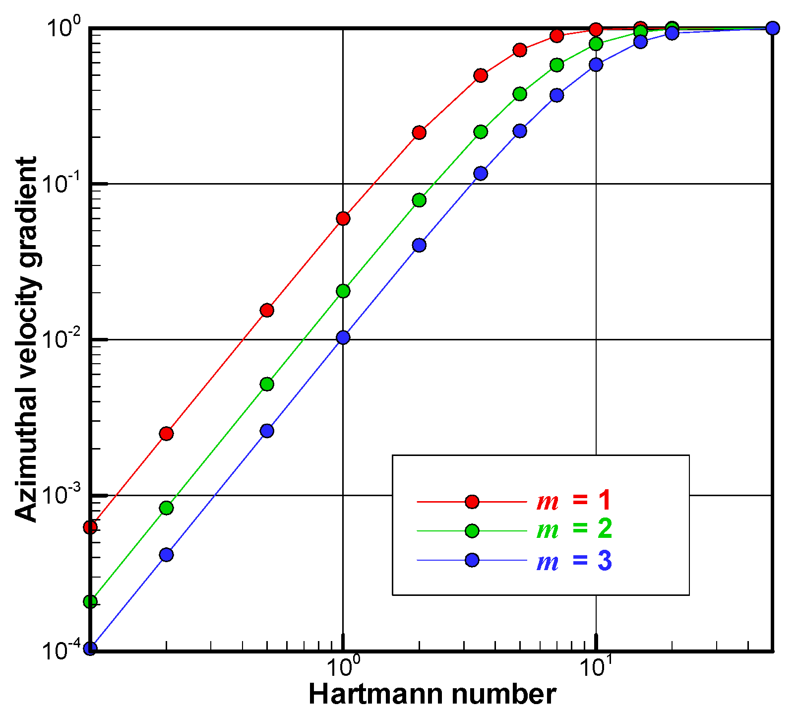
Figure 4 shows the azimuthal velocity gradient of the core flow at the axis of the cylinder for the three different cases of the number of pole-pairs. The azimuthal velocity gradient at the axis is proportional to the square of the Hartmann number for the cases of
Ha << 1. The azimuthal velocity gradient at
m = 1 is always larger than that at
m = 2 or 3. This means that the rotating magnetic field with
m = 1 is more efficient to drive the azimuthal flow than that with
m = 2 or 3.
3.2. Disturbance Equations
The basic velocity is not always realized, but it tends to become unstable for the higher values of the rotational Reynolds number. The present boundary layer flow along the concave surface is subjected to centrifugal instability. Therefore, toroidal vortices aligning along the axial direction are formed within the boundary layer near the sidewall. We assume that the perturbed components are axisymmetric and are superposed with the basic state as follows:
where the basic velocity and pressure are expressed as follows:
Then, we can obtain the linearized perturbation equations and boundary conditions as follows:
The boundary conditions for the perturbed components are given as follows:
The normal modes of the form are as follows:
where,
α is the axial wavenumber which is real number, and
s is in general the complex number. In this study,
s is assumed to be a real number and is regarded as the growth rate of the disturbance since the stationary state at the onset of secondary flow is focused. If
s > 0, the basic flow is unstable enough to generate the secondary flow. If
s < 0, the basic flow is stable since the disturbance attenuates as time evolves. Using Equation (49), we can obtain ordinary differential equations for a neutral state of the onset of secondary flow in a dimensionless form as follows:
where,
k is the dimensionless axial wavenumber,
Re is the rotational Reynolds number based on the angular velocity of the rotating magnetic field, and the dimensionless dependent variables such as velocity, pressure and electric potentials are as follows.
where,
D and
represent the differential operators, which are defined as
D =
d/
dR and
=
d/
dR + 1
/R respectively. The non-dimensional boundary conditions for the amplitude functions are as follows:
For a given wavenumber and Hartmann number, the simultaneous ordinary equations are numerically solved together with the above boundary conditions to obtain the neutral Reynolds number at which the basic flow becomes unstable.
3.3. Numerical Strategy
The simultaneous ordinary Equations (50) to (55) were decomposed into their real and imaginary parts, respectively, and discretized on a one-dimensional equidistant staggered grid system, as shown in
Figure 5. All the equations are discretized by the fourth order central difference method. The radial velocity is defined at cell boundaries, while the other variables such as the azimuthal and axial components of velocity and the pressure are defined at cell centers so as to satisfy the equation of continuity. The pressure is obtained by the HSMAC method [
35]. The computational procedure is as follows. First, for a given number of pole-pairs
m and Hartmann number
Ha, the basic flow profile such as the azimuthal velocity and the pressure is numerically obtained by solving Equation (37). Then, for a given wavenumber
k, its corresponding neutral Reynolds number can be obtained by using the Newton–Raphson method with Equations (50)–(55) during in which normalization of the amplitude functions is implemented in order to set them uniquely. In this study, a component of velocity at a certain point is fixed at unity during the computation. Such procedures are repeated by changing the value of
k. Among the various values of
k, the smallest value of the neutral Reynolds number is the critical Reynolds number.
3.4. Results
Table 1 shows the critical Reynolds numbers obtained for the various values of Hartmann number (
Ha) and number of pole-pairs (
m). The number of grids for all the analyses is 201, although the boundary layer formed in the vicinity of the side wall tends to be thin the Hartmann number increases. The dependency of the number of grids is quite small. For example, the critical values for
m = 2 and
Ha = 100 are
kc = 44.03 and
Rec = 2590.83 when the number of grids is 401. Even in this quite high Hartmann case, the discrepancy between the two different systems of grid is small. For low values of Hartmann number, the critical Reynolds number depends significantly on the number of pole-pairs. However, this tendency is not observed for high values of Hartmann number. For each case of the number of pole-pairs, there is a Hartmann number that takes the minimum critical Reynolds number. These values are approximately 425, 505 and 591 for
m = 1, 2 and 3, respectively.
Figure 6 shows the critical Reynolds numbers and their corresponding axial wavenumbers as a function of Hartmann number for the three cases of magnetic pole-pairs. For the case of low Hartmann number (
Ha << 1), the critical Reynolds number is proportional to
Ha−2 irrespective of the value of
m. Hence, the value of
Ha2 Rec takes a constant value depending on the value of
m. Both critical Reynolds number and critical wavenumber take almost the same value irrespective of
m for
Ha > 25 since the basic core flow is synchronized with the phase velocity of the rotating magnetic field.
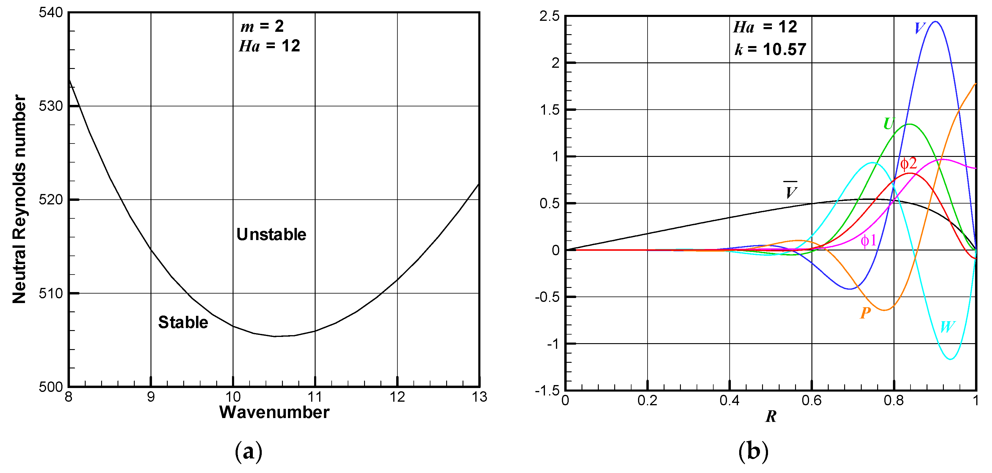
Figure 7 shows the neutral Reynolds number as a function of axial wavenumber for
Ha = 12 and
m = 2 (
Figure 7a) and each amplitude function at the critical point in which the axial wavenumber is 10.57 (
Figure 7b). The region below the curve indicates the stable region while that above the curve is the unstable region and, therefore, the secondary flow takes place. For
Ha = 12 and
m = 2, the Reynolds number takes its minimum value (
Rec = 505.36) at
k = 10.57. On the right-hand side figure, normalization of amplitude functions is made so that
U = 1 at
R = 0.9.
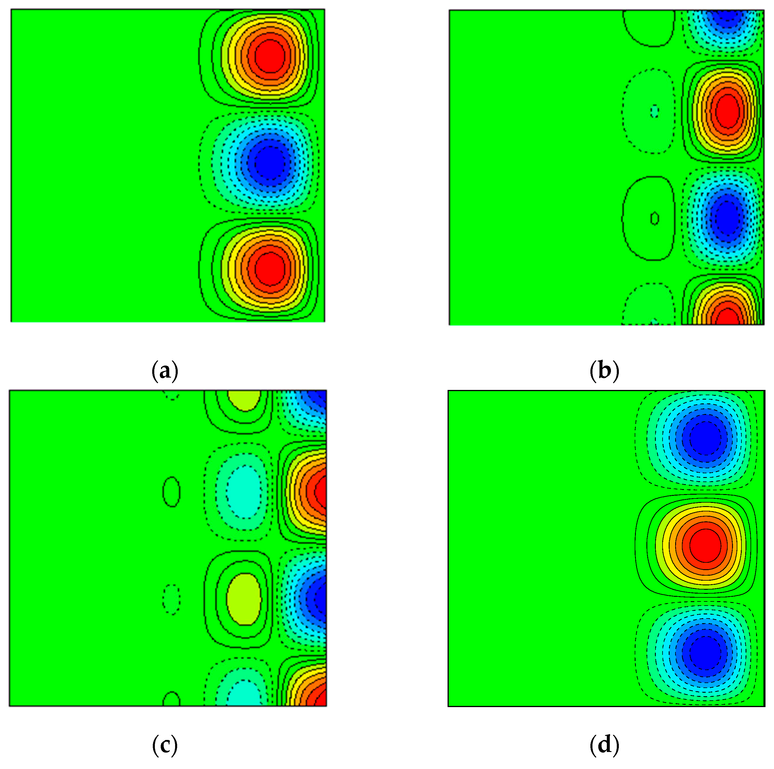
Figure 8 shows the visualization of the eigenfunction at the onset of instability for which the minimum critical Reynolds attained. These figures imply that there are almost three vortices aligned along the axial direction. It is quite interesting that the distribution of the Stokes’ stream function is similar to that of the electric potential (
φ2).
4. Discussions
4.1. Magnetic Taylor Number
Table 1 indicates that the value
Ha2Re in the limit of the small Hartmann number is 5834.0, 16182, and 34349 for
m = 1, 2, and 3, respectively. In this section, we consider the reason why these values approach each constant value in the limit of the small Hartmann number. First of all, the basic flow in the limit of the small Hartmann number is approximated as follows:
From Equation (58), the basic flow is proportional to the square of the Hartmann number. This solution can be obtained using Equation (59) in which the term of
in Equation (37) is neglected.
This implies that Ohm’s law, see Equation (6), is approximated using the following equation in which the induced electromotive force (
u ×
B) is dropped.
Then, Equation (58) is substituted into Equations (51), (52) and (53), neglecting terms including
Ha2, and the following simplified equations are obtained.
where, the magnetic Taylor number is defined as follows:
Eliminating the axial velocity by using Equations (50) and (63), and combining with Equation (61), we get the following equation without the expression of pressure:
Richardson [
2] used Equations (62) and (65) for
m = 1 in his analysis. According to his results, the critical magnetic Taylor number is 729.25 and the critical wavenumber is 6.59. The present numerical result for
m = 1 in the small limit of the small Hartmann number shown in
Table 1 is consistent with this result.
4.2. Validation of the Results
For the low Hartmann number cases, the values of the shielding parameter are estimated by using
Table 1. The magnetic Prandtl number for most liquid metals is in the order of 10
−6 and we use this value for the estimation. When
Ha = 0.01,
Rω =
Prm Re = 58.34 for
m = 1 and 343.5 for
m = 3. This implies that the fast rotating magnetic field hardly penetrates into the conducting fluid due to the significant skin effect. Therefore, these results would not be realized in a real system. When
Ha = 0.1,
Rω =
Prm Re = 0.5834 for
m = 1 and 3.435 for
m = 3. In these cases, the magnetic field can penetrate the conducting fluid to some extent but the skin effect is still obvious. When
Ha = 1,
Rω =
Prm Re = 0.006 for
m = 1 and 0.03 for
m = 3. In this case of Hartmann number, the skin effect can be neglected. The critical magnetic Taylor number is 761.9 for
m = 1 and 722.2 for
m = 3. These values are slightly larger than those of the low Hartmann number approximation discussed
Section 4.1. This implies that the magnetic Taylor number is not useful for the determination of the onset of secondary flow but the rotational Reynolds number appears to be considered for each given Hartmann number.
On the contrary, for high Hartmann number cases, the interaction parameter N = Ha2/Re, which is the ratio of the electromagnetic force to inertial force, becomes large. We should be careful about the value of N. For the case N >> 1, it would be difficult to keep an axisymmetric circular flow. For example, for m = 1 and Ha = 100, the value of N is approximately 3.8, the assumption of axisymmetric flow in this study would not be valid. However, for m = 1 and Ha = 9, the value of N is approximately 0.19. In this case, the assumption of axisymmetric flow is valid since the basic azimuthal flow does not synchronize with the speed of the rotating magnetic field.
4.3. Influence of Eelectric Potential
In this subsection, we discuss the influence of the electric potential that appeared in Ohm’s law, which governs the electric current density.
Table 2 shows the comparison of the critical Reynolds number for various Hartmann numbers with and without taking the electric potential into account at
m = 1 [
36]. When the Hartmann number is very small, since the term of the time-derivative of the vector potential is far superior to that of the induced electromotive force, the divergence-free condition for the electrical current density is automatically satisfied due to the employment of the Coulomb gauge. Therefore, the electric potential does not seem to be generated. As seen in
Table 2 for the low values of Hartmann number, the difference of the critical Reynolds number and its corresponding wavenumber between the cases with and without the electric potential is negligible. However, for the high values of the Hartmann number, the difference between the two cases is significant. The electric potential makes this flow more unstable.
5. Non-Linear Computations
So far we have focused on the onset of secondary flow instability driven by the rotating magnetic field for an infinitely long cylinder case without taking the end effect into account. For the application of crystal growth of a semiconductor or other metal processes, it would be necessary to consider the end effect, as well as the aspect ratio of the height to the radius of the cylinder. Such discussion requires non-linear direct numerical computation. In this section, we focus on the influence of the boundary condition at the bottom and top walls on the supercritical flow for a finite cylinder case.
5.1. Periodic Condition
In this section, a periodic boundary condition is considered to compare with the results obtained in the linear stability analyses. The boundary conditions employed for the periodic condition are shown in Equation (66).
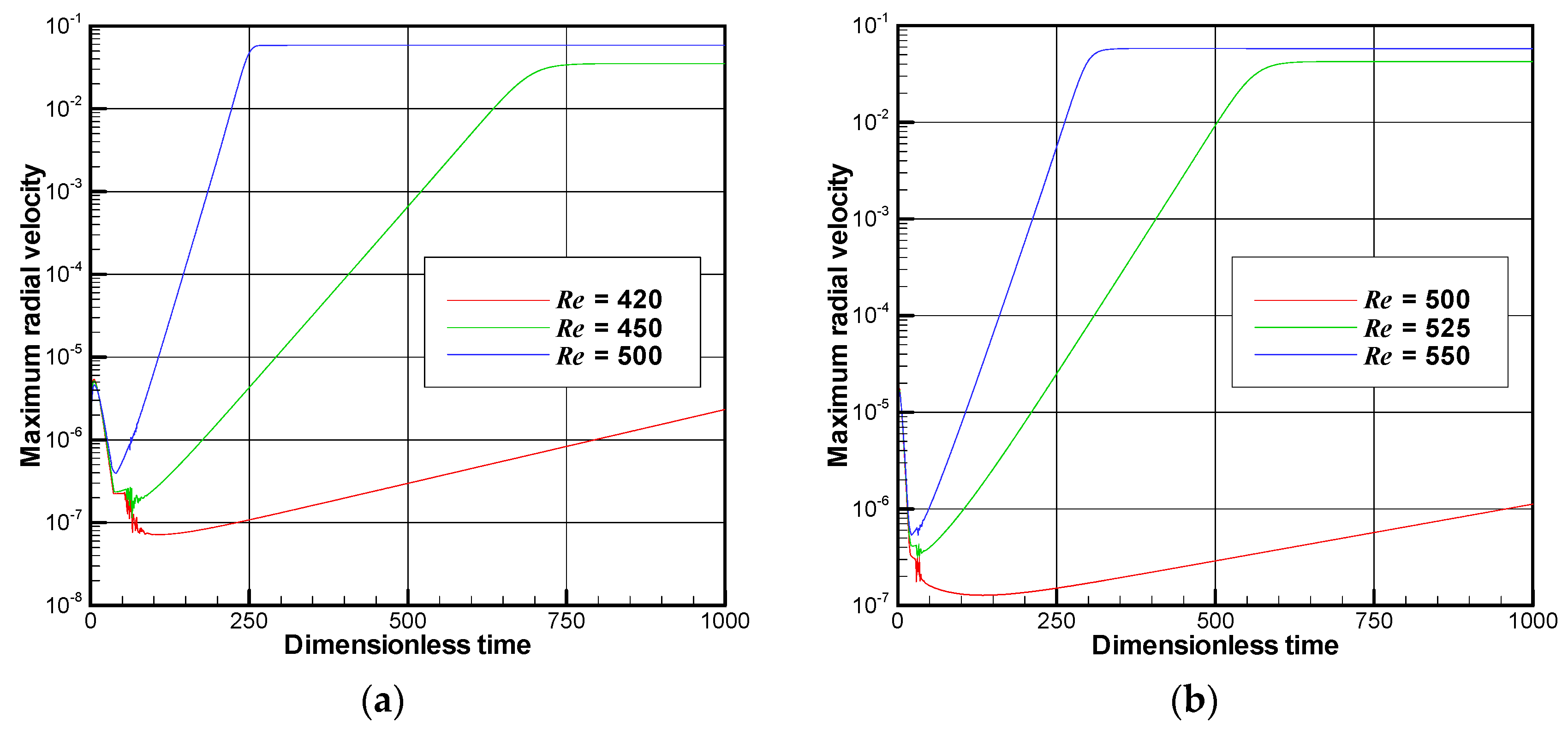
Figure 9 shows the growth rate of the maximum radial velocity for several values of the Reynolds number for the aspect ratio
A = 1,
m = 1 and
Ha = 9 or 16. The number of grids employed is 129 × 129 in the radial and axial directions, respectively. At the beginning of computation, each curve exhibits unpredictable behavior but it soon grows exponentially until the non-linear effect becomes significant. The critical Reynolds number obtained by the linear stability analysis for
m = 1 and
Ha = 9 is approximately 425, but the present non-linear analysis indicates that the growth rate at
Re = 420 is slightly positive. The same contradiction occurs at
Ha = 16. This discrepancy between the linear and non-linear analyses may be due to the difference in the number of grids employed as well as the difference in the wavenumber. The critical wavenumber predicted by the linear analysis is about 9.26, while the wavenumber by the non-linear analysis is equivalent to about 9.42 because there are three vortices aligned within the cylindrical enclosure for
A = 1.
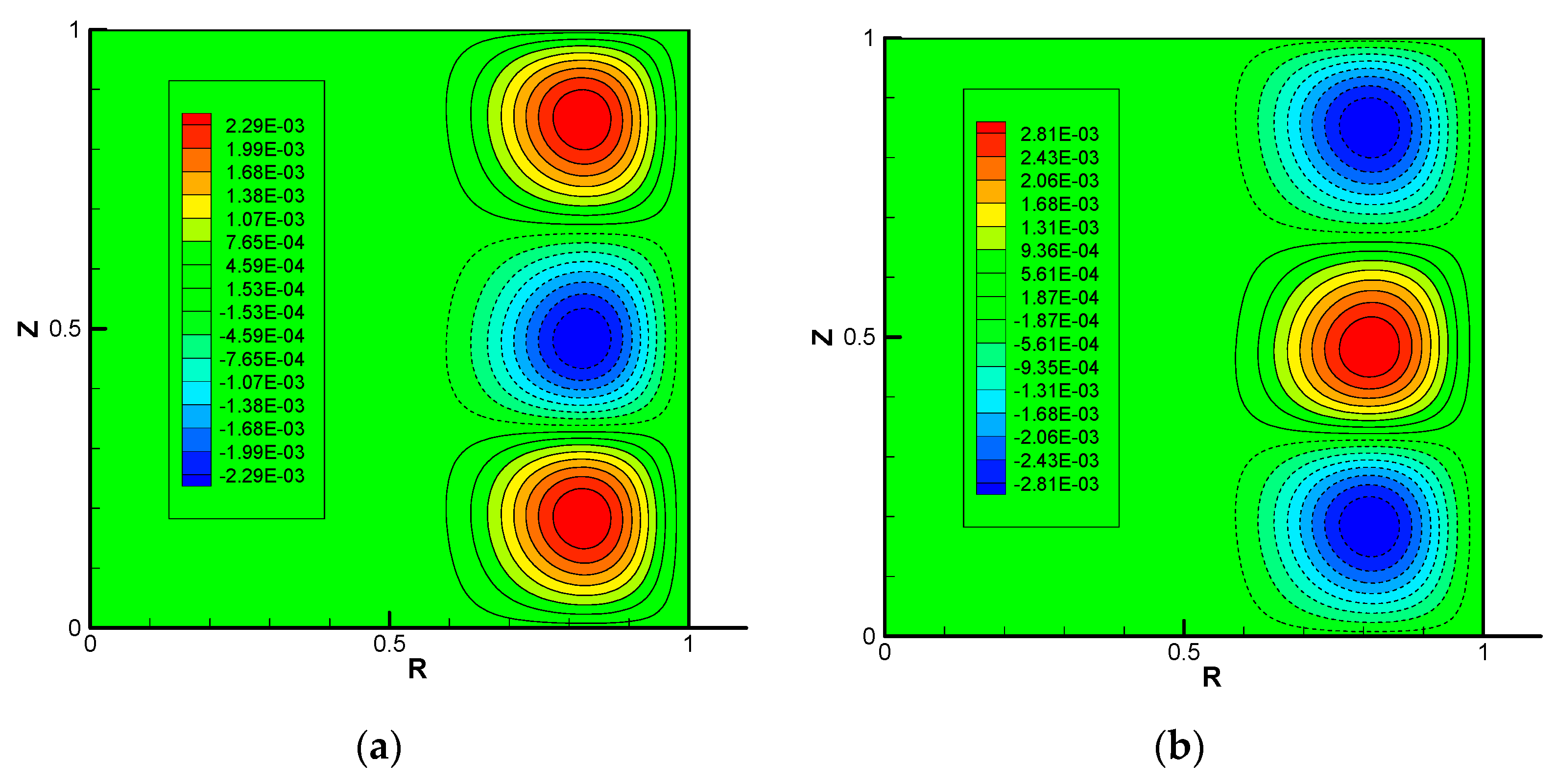
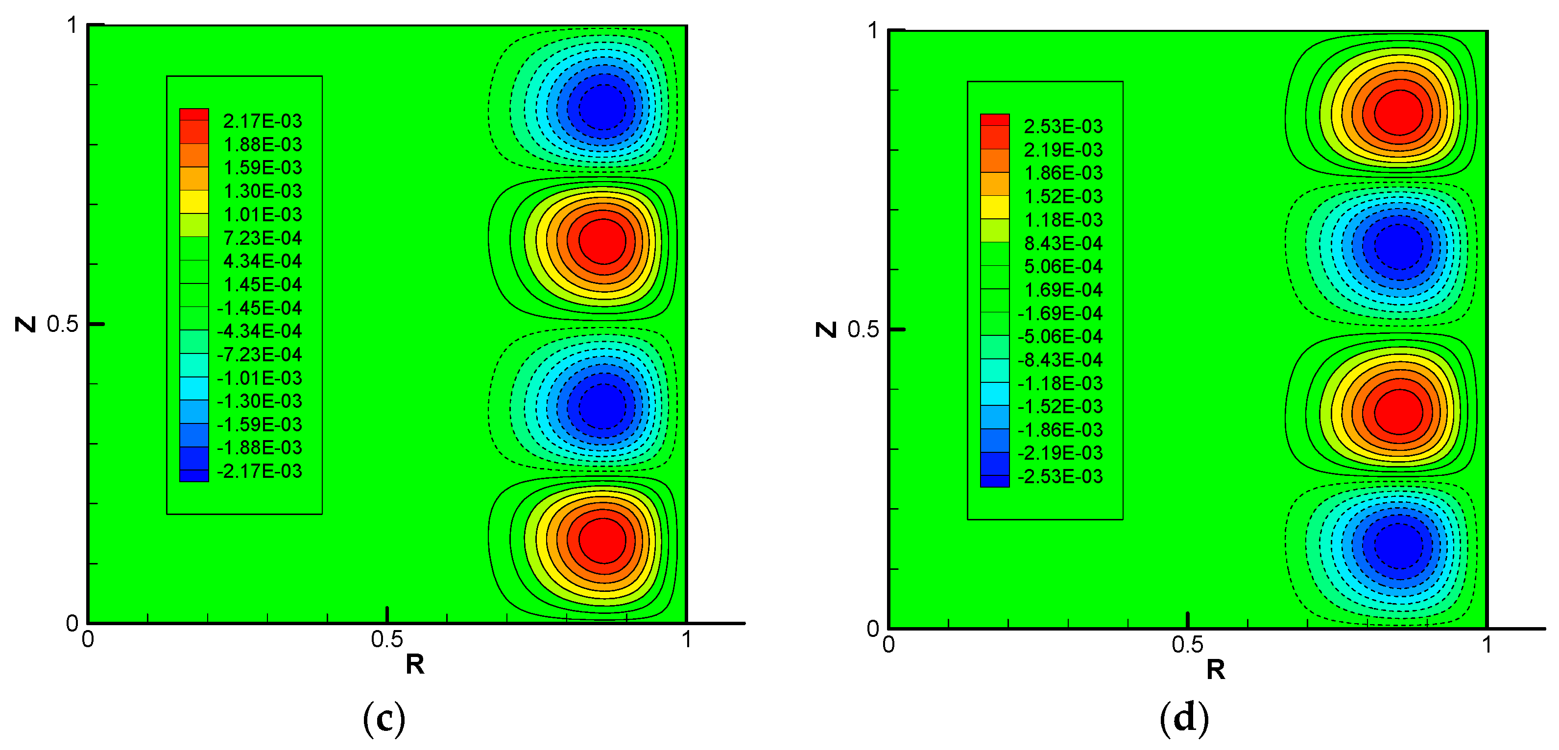
Figure 10 shows contour lines of the Stokes stream function and the electric potential
Φ2 for the two different cases at the steady state that includes the non-linear effect. Since the value of Reynolds number is slightly higher than the critical condition, the fields of flow and electric potential are compared with
Figure 8 for
m = 1 and
Ha = 9. Due to the non-linear effect, which indicates that the perturbed flow is large enough to interact with the basic flow, the shape of the vortices is evidently distorted. However, the number of vortices is coincident between the linear and non-linear computations if the number of pole-pairs
m and the Hartmann number
Ha are the same within this range of the Reynolds number
Re.
5.2. No-Slip Condition for A = 2
In this section, computational results with a no-slip condition at the top and bottom walls are discussed in order to compare with those with the slip condition. The effect of the aspect ratio would be crucial, but we would restrict the results only to
A = 2. The most striking difference from the slip condition is that the basic flow with the no-slip condition has always been the secondary flow.
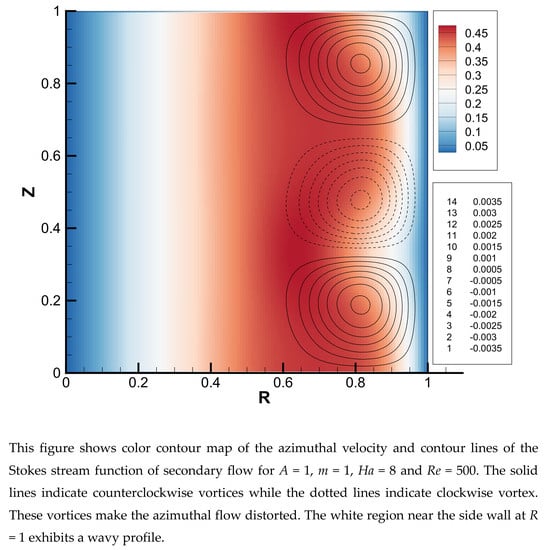
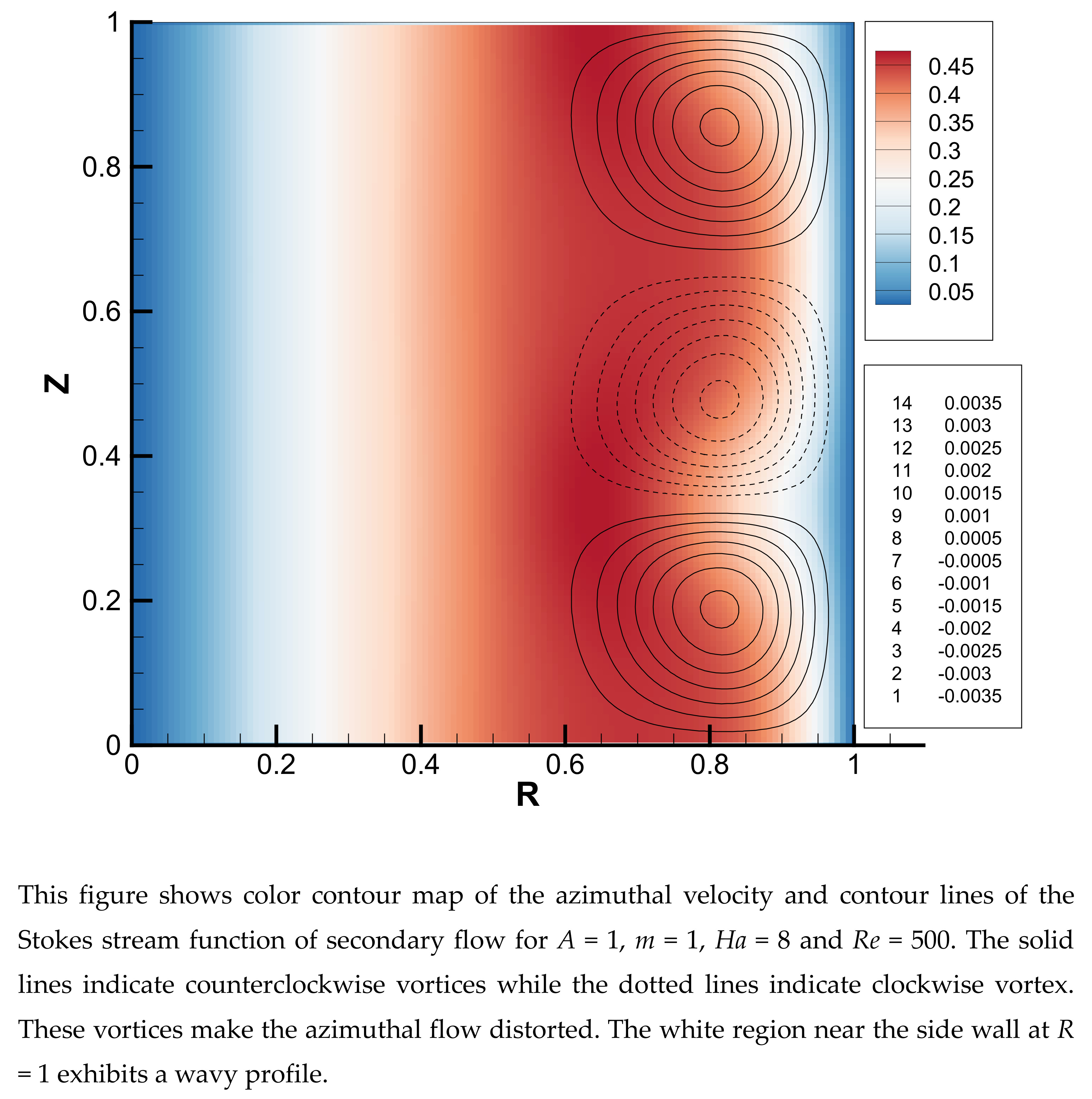
Figure 11 shows the contour maps for
m = 1 and
Ha = 8 for the three different values of Reynolds number. The upper ones show the azimuthal velocity whereas the lower ones show the Stokes stream function. In the case of the no-slip condition at the top and bottom walls, the secondary flow has two large vortices when the Reynolds number is not very high. As the Reynolds number increases, the boundary layers formed in the vicinity of the side wall and that of the top and bottom walls become thin. Steady solutions were obtained until a Reynolds number of about 5000 for
Ha = 8, beyond which the flow becomes unsteady. In the unsteady case, as shown in
Figure 11c, a radially inward flow is observed at the mid-height of the side wall. However, this oscillatory flow is almost symmetrical with respect to
Z = 1 (mid-height).
Figure 12 shows the contour lines of the azimuthal velocity for various combinations of the Hartmann number and the Reynolds number when the number of pole-pairs is 1. As indicated in the previous figure, the flow transits from steady to unsteady as the Reynolds number increases but its value significantly depends on the Hartmann number. These Reynolds numbers indicate the approximate critical value above which the flow becomes oscillatory. The quasi-critical values are much larger than the critical values shown in
Table 1 if the same Hartmann numbers are compared. Surprisingly, the azimuthal profiles are quite similar to each other, although the maximum azimuthal velocity, the value of which is written in each figure, is quite different. The common feature of this velocity profile is that there are oscillatory regions in the vicinity of the top and bottom walls. In this no-slip condition case, the top and bottom walls are stationary while the flow is mainly rotating in the azimuthal direction. Therefore, the Bödewadt boundary layer [
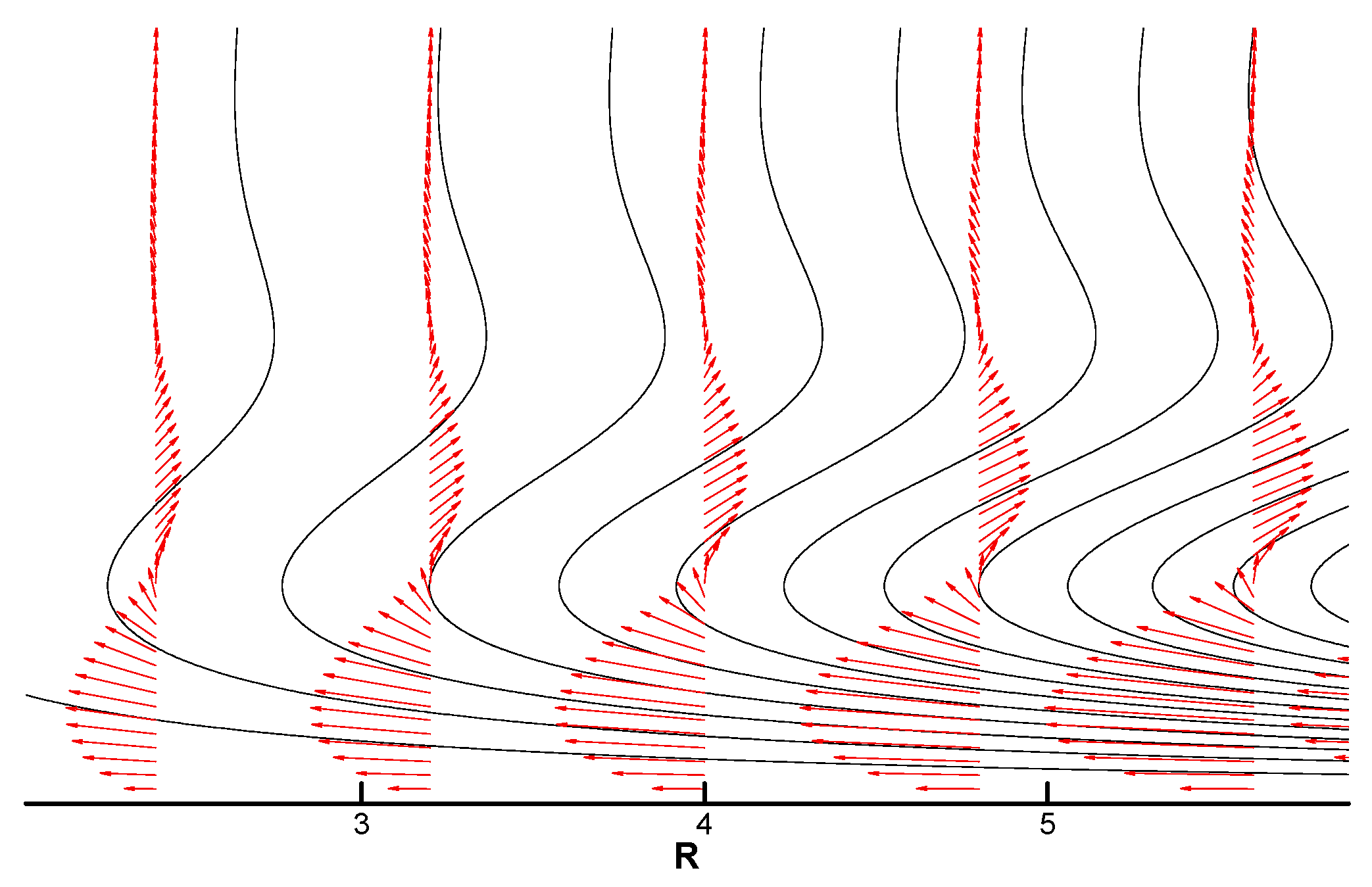
37], which is known to exhibit an oscillatory profile, should be formed both in the vicinity of the top and bottom walls.
Figure 13 shows the Bödewadt boundary layer obtained numerically by an additional computation assuming a similar solution. By comparing
Figure 12 and
Figure 13, it is recognized that the Bödewadt boundary layer is approximately formed except in the region near the side wall where the adverse azimuthal velocity gradient is observed.
6. Conclusions
In this paper, the flow of the electrically conductive fluid in the cylindrical vessel driven by a multi-pole rotating magnetic field was discussed by using the linear stability analyses and non-linear direct numerical computations. The following conclusions were obtained.
1. For the cases in which the shielding parameter (magnetic Reynolds number) was much smaller than unity, the skin effect (induced magnetic field) was negligible. For such cases, the mathematical modeling of the rotating magnetic field with the arbitrary number of pole-pairs was derived.
2. Decomposition of the electric potential into two parts allows us to derive the averaged electromagnetic force including potential gradient terms together with the assumption of the axisymmetric flow field.
3. For the infinitely long cylindrical vessel, the basic flow which has only an azimuthal component of velocity is not influenced by the electric potential. When the Hartmann number is very small, the influence of the number of pole-pairs on the basic flow is significant. When the Hartmann number is large, the dependency of the number of pole-pairs decreases and the angular velocity, except for at the boundary layer in the vicinity of the sidewall, synchronizes with the angular velocity of the rotating magnetic field.
4. For the low Hartmann number cases, the flow cannot follow the angular velocity of the rotating magnetic field. In such cases, the magnetic Taylor number determines the threshold of the onset of the secondary flow. This implies that both terms of the induced electromotive force and the potential gradient in Ohm’s law can be neglected compared to the time-derivative of the vector potential. However, since it requires a very high angular velocity to generate the visible flow, the skin effect sometimes has to be taken into account.
5. For arbitrary cases of the Hartmann number, the Reynolds number based on the angular velocity of the rotating magnetic field determines the threshold of the onset of secondary flow instead of the magnetic Taylor number. In addition, there exists a certain Hartmann number that takes the minimum value of the critical Reynolds number, and its value depends on the number of the pole-pairs.
6. For the high Hartmann number cases, since the angular velocity of the magnetic field and the flow field are substantially synchronous, both terms of the induced electromotive force and the potential gradient in Ohm’s law are significant. When the interaction parameter was much larger than unity, the electromagnetic force was superior to the inertia force, it appears that the axisymmetric circular flow might not be established. A non-axisymmetric time-dependent model may be required for such cases.
7. The non-linear direct computation suggests that the magnitude of the velocity component of the secondary flow increases exponentially as time evolves, and the growth of disturbances eventually stops after the non-linear effect becomes apparent and the velocity component becomes constant. Comparing the results between the linear stability analysis and non-linear direct computation, both results were in good agreement in terms of the critical value and the wave number.
8. The case with the no-slip boundary condition forms the Bödewadt boundary layer near the top and bottom walls and the basic flow includes the secondary flow. The stability of this case would depend on the aspect ratio; however, generally, it was much more stable than the flow with slip condition.


