Abstract
In neutral fluids and plasmas, the analysis of perturbations often starts with an inventory of linearly unstable modes. Then, the nonlinear steady-state is analyzed or predicted based on these linear modes. A crude analogy would be to base the study of a chair on how it responds to infinitesimaly small perturbations. One would conclude that the chair is stable at all frequencies, and cannot fall down. Of course, a chair falls down if subjected to finite-amplitude perturbations. Similarly, waves and wave-like structures in neutral fluids and plasmas can be triggered even though they are linearly stable. These subcritical instabilities are dormant until an interaction, a drive, a forcing, or random noise pushes their amplitude above some threshold. Investigating their onset conditions requires nonlinear calculations. Subcritical instabilities are ubiquitous in neutral fluids and plasmas. In plasmas, subcritical instabilities have been investigated based on analytical models and numerical simulations since the 1960s. More recently, they have been measured in laboratory and space plasmas, albeit not always directly. The topic could benefit from the much longer and richer history of subcritical instability and transition to subcritical turbulence in neutral fluids. In this tutorial introduction, we describe the fundamental aspects of subcritical instabilities in plasmas, based on systems of increasing complexity, from simple examples of a point-mass in a potential well or a box on a table, to turbulence and instabilities in neutral fluids, and finally, to modern applications in magnetized toroidal fusion plasmas.
1. Introduction
Subcritical instabilities are nonlinear instabilities that occur even as the system is linearly stable, but with a threshold in the amplitude of initial perturbations. Subcritical instabilities stay dormant until they are brought over their threshold by some interaction, drive, forcing, or even thermal noise or other naturally occuring perturbations if the threshold is low enough. Subcritical instabilities are ubiquitous in neutral fluids and in plasmas. They are of great interest due to their essential impact on the onset of turbulence, structure formation, anomalous resistivity, and potentially, turbulent transport. Indeed, the widespread use of linear theory which subcritical instabilities circumvent as a fundation of nonlinear (or quasi-linear) theories is a major caveat in the conventional analysis of wave-like perturbations. The growth of subcritical instabilities is a nonlinear process, which is often independent of their linear decay rate. They open a new channel for tapping free energy.
In plasma contexts, developments in the theory of subcritical instabilities have been ongoing since the late 1960s. The physical mechanisms of nonlinear growth are multiple, but subcritical instabilities share common features in terms of bifurcation, and in terms of their macroscopic impact, which are typically equivalent or larger than the impacts of linearly unstable perturbations. The growth mechanisms are well documented, and theories often yield accurate analytic formulas for their amplitude thresholds and for their nonlinear growth rates.
Direct measurements in neutral fluid experiments have confirmed the existence and importance of subcritical instabilities. In plasmas, fluid-like subcritical instabilities have been well documented in laboratory experiments. However, high-temperature plasmas feature other kinds of instabilities that involve non-Gaussian distribution functions. Direct measurements of these kinetic subcritical instabilities are more difficult, because they are often based on short-lived structures with small scales in both real space and velocity space (but which together yield macroscopic, long-lived impacts on magneto-hydrodynamics). The development of new techniques to obtain more accurate measurements of phase-space density are ongoing.
Subcritical instabilities can be approached from various standpoints. Large parts of the literature focus on the mechanisms by which a finite amplitude seed perturbation can grow nonlinearly or how the nonlinear structure sustains itself. Several scenarios for the onset of subcritical instabilities or the subcritical transition to turbulence have been uncovered. In some cases, infinitesimal perturbations or noise can grow transiently, either into a finite amplitude seed or directly into a self-sustained nonlinear structure. In other cases, large enough seeds can be formed by external forcing or by an avalanche process originating from a linearly unstable region (which can be a region in space-time). Dauchot and Manneville described the concept of subcritical instability from the point-of-view of a local versus global analysis of stability [1]. Based on a simplified model of Navier–Stokes turbulence, they showed that stability conditions can only be determined from the knowledge of all reachable attraction basins rather than from the stability of the local basin. Yoshizawa, Itoh, and Itoh described the topic of subcritical instabilities based on examples of plasma instability, as can be found in their textbook [2]. Nonmodal stability theory, as reviewed by Schmid [3], has been successfully applied to the analysis of nonlinear stability over a wide range of fluid and plasma contexts, including space-and-time-dependent flows in complex geometries.
In this paper, which is based on a tutorial that was published in Japanese only [4], we attempt to describe the basic concepts of subcritical instability, starting from the simplest example of a point mass in a potential well, and then building up to increasingly complex physical contexts: the Kelvin–Helmholtz instability, quasi-2D and pipe flows, 1D plasma, drift-waves in magnetized plasmas, and finally, strong electro-magnetic bursts driven by energetic particles in magnetized toroidal plasmas. We do not attempt to present a review of the literature on subcritical instabilities and subcritical turbulence, but rather, propose an introduction of the topic by selecting a few paradigmatic examples. The aims are two-fold: (1) to allow the reader to get a clear physical picture of some of the various mechanisms by which subcritical instability can occur and (2) to point out interesting analogies between neutral fluids and plasmas which may be exploited to push the research further.
2. Concepts of Subcritical Instability
Let us set up a simple model of Newtonian mechanics to illustrate the concept of subcritical instability by analogy.
Consider a point mass of radial coordinate r resting on a surface of altitude or equivalently, a positively charged particle in an electric potential , where
Here, a, b, and c are constant input parameters which characterize the shape of the potential. Let us assume that the point mass or particle is initially at and is ultimately bounded to a finite r region of space, which is imposed by the condition . In this section we arbitrarily choose . We consider two qualitatively different cases for b, namely and . As we will argue in this paper, these two cases represent systems which can () or cannot () feature subcritical instabilities.
Figure 1a shows the potential for , , and and a point mass or charged particle after it has been perturbed by an external push towards positive r. This corresponds to conventional, supercritical instability. We assume that there is some form of energy dissipation. Any initial perturbation in r will grow linearly at first, and then r will oscillate around the stable equilibrium, before reaching the latter equilibrium in the time-asymptotic steady-state. In contrast, Figure 1b shows the potential for , , and , which is linearly stable but nonlinearly unstable. If the initial perturbation is small enough, the point mass or particle will oscillate around with its amplitude decreasing over time until it returns to rest back at its original location. If the push is large enough, on the contrary, the point mass or particle will overcome the potential barrier and reach another potential. In doing so, it will extract free energy that would not be available if it did not overcome the potential barrier. This qualitatively illustrates the basic concept of subcritical instability. Next, we perform a quantitative analysis.
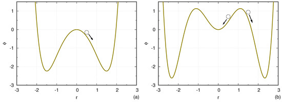
Figure 1.
Cartoon of the concept of supercritical and subcritical instabilities. The solid curve is a fixed potential. (a) Supercritical case: , , and . The equilibrium is unstable. (b) Subcritical case: , , and . The equilibrium is stable to small perturbations (circle and arrow at ) but unstable to perturbations with an amplitude above a certain threshold (circle and arrow at ).
Figure 2a,b show the potential for the two cases and and for various values of a ( as before). In both cases, in the neighborhood of , the potential is strictly concave for any and strictly convex for any . The equation of motion is
where K is a positive constant. The linearized equation of motion is . Therefore, a linear analysis informs us that the equilibrium is stable for , unstable for , and marginal for . In other words, the linear instability threshold is simply . For , the linear growth rate is proportional to .
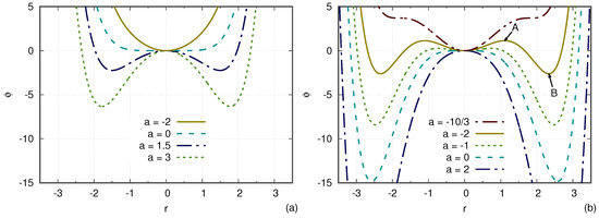
Figure 2.
Potential for various values of a. We recall that a is proportional to the square of the linear growth rate. (a) Supercritical case: . (b) Subcritical case: . Two points are shown by arrows: point A is the potential barrier at and point B is the saturated value for the subcritical instability, .
A nonlinear analysis, in contrast, yields a much different story. The equilibrium states are given by and r such that . The slope of the potential is
which cancels out for and 0, 2, or 4 other real solutions, depending on the values of b and . Let us focus on the case where .
- If , there is no other real solution than .
- If (which is only relevant for ), there are four real solutions other than , which are and . Here,andThe second derivative of the potential at these solutions is, straightforwardly,andTherefore, with our initial assumption of , and . This proves that are unstable equilibria, while are stable equilibria, as can be seen from the plot of in Figure 2b.
- Finally, if , there are two real solutions other than , which are .
Let us summarize how this translates in terms of stability for two qualitatively different systems: and . For , if , the only equilibrium, , is stable. If , the equilibrium is unstable, and there are two attraction basins, and , which are stable. This corresponds to the conventional linear instability followed by nonlinear saturation, where, in the analogy, r is the amplitude of fluctuation.
For , if , the situation is qualitatively similar to the case , . We recover the same two attraction basins, , which are easily reached because is concave at . However, if , there are three stable equilibria: , , and . Starting from the location , the point mass or the particle can reach one of the two other attraction basins if it overcomes the potential barrier peaking at . This corresponds to the subcritical instability.
From the latter analysis, one can determine the conditions for instability in bifurcation diagrams such as Figure 3a for the system with and Figure 3b for the system with . In terms of the bifurcation theory, the system with features a supercritical Hopf bifurcation, and the system with features a subcritical Hopf bifurcation (at ) as well as a fold bifurcation (at ). The unstable equilibria are also thresholds that must be reached to trigger the instability. The stable equilibria are also the saturated amplitudes. As we will see, the “finger” shape in Figure 3b is typical of subcritical instabilities in neutral fluids and in plasmas. Note that while linear stability is given by a condition on a 1D parameter space (a), nonlinear stability is given by a condition on a 2D parameter space (a, r).
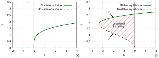
Figure 3.
Bifurcation diagram, which yields the nonlinear stability. The solid curves are the stable equilibria and , which correspond to the saturation amplitude. The dashed curves are the unstable equilibria and , which correspond to the threshold amplitude. (a) Supercritical system: . (b) Subcritical system: . The region of subcritical instability is shown by hashes. The same points (A and B) as in Figure 2 are shown by arrows in this figure as well.
These subcritical bifurcations have crucial implications, not only for linear theories, but also for nonlinear theories that are based on an expansion in the perturbation amplitude. Indeed, in the system where subcritical instabilities are absent, an argument of near-marginality is often made: the system naturally remains near linear marginality (), because if the conditions overcome linear marginality (), the instability will tend to counteract the source of instability, bringing the system back to . Now, in the system , the same argument does not stand for two reasons: (1) near marginality (), the perturbation has a finite amplitude ; and (2) if the conditions overcome linear marginality, the instability will counteract the source, bringing a not only back to but even to a finite negative value of the order of , which may be far from marginal stability.
Finally, let us mention the existence of a third paradigm. A system can feature subcritical instabilities, even if there are no linear instabilities for any finite value of the control parameter. As an example, we can consider a solid box placed on a plane surface (an idealization of a cup on a table). The box has a square base of length l and height h. Figure 4 shows the box tilted by an angle and the potential energy which is then proportional to . As the parameter increases, the potential well at becomes shallower and narrower but never vanishes. Hence, the equilibrium is always linearly stable. However a subcritical instability can be triggered if the perturbation overcomes a threshold such that . Figure 5 shows the resulting bifurcation diagram. Here, there is no subcritical Hopf bifurcation (or one could argue that it has been pushed towards infinity), and the subcritical instability spans the whole parameter space.
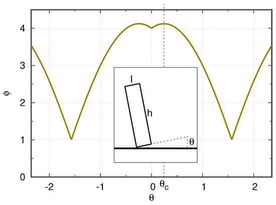
Figure 4.
Potential energy (normalized) for a box on a plane with height . Inset: cartoon of the setup where the box is tilted by an angle .
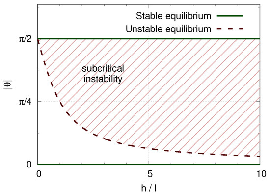
Figure 5.
Bifurcation diagram for a box on a plane. The dashed curve is the unstable equilibrium , which corresponds to the threshold amplitude. The region of subcritical instability is shown by hashes; it spans the whole range of finite values of the control parameter .
3. Subcritical Instabilities in Neutral Fluids
In fluid dynamics, the concept of subcritical instability is not to be confused with that of subcritical flow, which is defined as a flow with Froude number of less than 1 [5]. To the authors knowledge, subcritical flows and subcritical instabilities are unrelated. Subcritical turbulence, in particular, in the presence of sheared flow, has a long history of experimental [6,7,8,9], numerical [10], and theoretical research, as summarized in [11]. As entry points, we refer to a textbook by Drazin and Reid [12], partial reviews of transition to turbulence by Grossman [13] and Manneville [14], and an attempt at an historical review in Chapter 2 of Borrero’s Ph.D. thesis [15]. In this section, rather than attempting another review, we describe a few examples to introduce the reader to the relevant concepts that find counterparts or analogies in plasma flows. Firstly, the Kelvin–Helmholtz instability in 2D geometry (in a Hele–Shaw cell) provides a clear example of subcritical bifurcation. Secondly, the literature on Couette flow, Poiseuille flow, and flat plate laminar boundary layer provides a relatively simple example of the physical mechanisms of growth of a finite amplitude perturbation.
3.1. Experimental Measurement of Subcritical Bifurcation
Meignin et al. observed and characterized, with great clarity, a subcritical instability in experiments of the Kelvin–Helmholtz instability in a Hele–Shaw cell [16]. Figure 6 describes the experimental setup. Two fluids (nitrogen gas and oil here) were injected at the same pressure into a thin space between two parallel glass plates. The two fluids flowed out at atmospheric pressure. Here, the gas to liquid density ratio was of the order . The gas velocity was used as a control parameter that corresponded to the drive of the instability. A perturbation was applied via a periodic modulation of the oil injection pressure (keeping the pressure of both fluids equal, on average). This led to an observed sine wave (at the inlet) of vertical amplitude (“forcing amplitude”). Figure 7 shows the observation in three typical cases: damping (stable), marginal (steady), and growing (unstable).
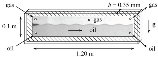
Figure 6.
Reproduced from [16]. Sketch of the experimental setup to study the subcritical Kelvin–Helmholtz instability in a Hele–Shaw cell. Nitrogen gas and silicon oil were injected from the left into a thin cell between two parallel glass plates. Gravity is shown by an arrow marked . An initial sine perturbation of the interface was imposed at the end of a splitter tongue where fluids met (left), and this was observed downstream (right).
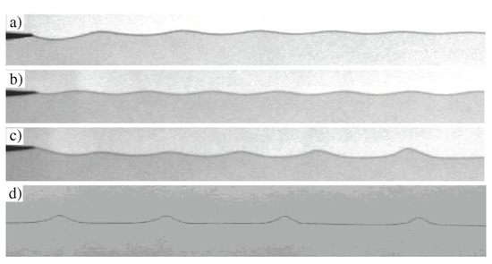
Figure 7.
Reproduced from [16]. The experimental results are shown. As the wave propagates, its amplitude is either damped (a), or constant (b), or amplified (c), depending on the initial amplitude and on the injection velocity. When the wave is amplified, it eventually saturates to a cnoidal-like wave, as shown in a picture taken far downstream (d).
For large enough values of gas velocity, they found a critical forcing amplitude below which the perturbation was damped, but above which the perturbation grew until it saturated to a larger value. This threshold in forcing amplitude is shown by open circles in Figure 8. The saturation value is shown by filled circles. From this figure, it can be concluded that linear instability is given by a simple condition, , where m·s. In contrast, nonlinear instability extends to a larger domain, given by two conditions, , where m·s and . The unstable region is marked by up arrows in the figure. The part of the unstable region where is the region of subcritical instability. Note the striking similarity with Figure 3b. A similar diagram is found for a wide range of fluid applications, including increasingly complex systems such as the Taylor–Couette cell of polymer solutions [17]. A specific introduction for subcritical instabilities of visco-elastic polymers flows is available [18].
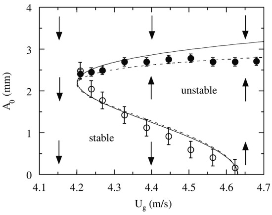
Figure 8.
Reproduced from [16]. Nonlinear stability diagram in the space of the forcing amplitude against the gas velocity (instability drive). The open circles show the amplitude threshold for the subcritical instability. The filled circles show the saturation amplitude. The curves are fits of the experimental results by a reduced theoretical model. See the reference for details.
In the Kelvin–Helmholtz case, as can be seen in Figure 8, the subcritical region extends by (in terms of ) into the linearly stable region. In the case of plane Poiseuille flow, the subcritical region extends by in terms of the Reynolds number into the linearly stable region (linear threshold , nonlinear threshold [19]). In the case of hot plasmas, we will see that this extension can be even more dramatic.
The existence of a subcritical instability in the case of two layers of immiscible, inviscid, and incompressible fluids in relative motion, which is an ideal limit of the latter experiment, was predicted qualitatively by Weissman [20]. The key point is the existence of nonlinear solutions. In addition, he showed that the nonlinear stability of an initial perturbation is sensitive to the form of the initial perturbation. We will be able to make many similar conclusions for hot plasmas.
Finally, subcritical turbulence can be strong enough to hide underlying linear instabilities. This is the case for Hagen–Poiseuille flow in slightly curved pipes [21].
3.2. Physical Mechanism of Subcritical Growth in Neutral Fluids
The physical mechanism of subcritical growth of a finite amplitude perturbation can take various forms depending on the system.
Let us first focus on two classical flows: plane Couette flow, and plane Poiseuille flow. The setups are illustrated in Figure 9. The plane Couette flow is the laminar flow of a viscous fluid between two parallel plates, one moving with respect to the other. The plane Poiseuille flow, on the other hand, can be seen as a limiting case of the plane Couette flow where the boundary plates are not moving. The flow is then driven by a pressure gradient imposed between the inlet and the outlet.
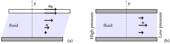
Figure 9.
(a) Cartoon of the plane Couette flow setup. A fluid is contained between two plates, both normal to the y-axis. The bottom plate is fixed, as illustrated by hashes. The upper plate is moving at a given velocity . (b) Cartoon of the plane Poiseuille flow setup. A fluid is contained between two plates, both normal to the y-axis and both fixed. The pressure is higher at the inlet than at the outlet.
In the case of planar Poiseuille flow, Henningson and Alfredsson proposed a mechanism called “growth by destabilization” [22], based on a more general suggestion by Gad-el-Hak [23]. In the growth by destabilization mechanism, a spot of finite amplitude fluctuations acts as a local obstruction that modifies the velocity profile in the vicinity of the spot. The modified profile is linearly unstable and allows the perturbation to grow. The modified profile was later confirmed experimentally by Klingmann and Alfredsson in the case of planar Poiseuille flow [24] as well as by Dauchot and Daviaud [25] in the case of the plane-parallel Couette flow, suggesting the validity of the mechanism of growth by destabilization.
To give an example of another mechanism, let us now focus on the flow in the laminar boundary layer near a flat plate. It was shown experimentally [26] and explained theoretically [27] that a convecting vortex moving at a fixed distance from the flat plate can drive instabilities in the free streaming flow when its translational velocity is a fraction of the free-stream velocity [28]. This instability can grow either upstream or downstream from the vortex, depending on the relative signs of vorticity between the mean field and the vortex structure. This suggests another mechanism of subcritical instability. Suppose that in some region of a flow, a linear instability generates a vortex. The vortex, which is an extremely coherent structure, may then travel without much distortion to a linearly stable region of the flow and, in turn, drive instabilities by extracting further energy from the mean flow. This latter mechanism of vortex-induced subcritical instability will be particularly important in plasma where there is a kinetic counterpart of fluid vortices.
In wall-bounded shear flows, subcritical transition to turbulence has been thoroughly investigated [29,30]. The whole process, called lift-up, is now fairly well understood, from the first local formation of finite amplitude perturbation, to its evolution towards three-dimensional structures and the self-sustaining mechanism of these structures [31,32]. Here, let us summarize the self-sustaining mechanism, assuming that the equilibrium fluid velocity is along the x axis and is sheared in the y direction, . The mechanism involves three main elements: (1) stream-aligned rolls sustain perturbations in the z direction of the parallel (streamwise) fluid velocity, , called streaks. (2) The latter streaks are linearly instable and lead to a 3D perturbation of the form . (3) In the nonlinear phase of this instability, the latter 3D perturbation self-interacts via convective acceleration and transfers its energy to the original stream-aligned rolls, closing the cycle. A similar mechanism was later found in pipe flow [33,34,35].
It should be noted that subcritical transition to turbulence often features co-existing laminar and turbulent regions. Localized turbulence may or may not expand globally, depending on the parameters. Pomeau proposed the concept of spatio-temporal intermittency to interpret these observations [36].
Subcritical instabilities are not limited to laboratory experiments. They have been proposed for shear instabilities of wave-driven, along-shore currents, first in an idealized situation [37], and then for a realistic configuration reproducing US coastlines and including the effects of eddy viscosity and bottom friction [38].
4. Subcritical Instabilities in Plasmas
We propose to categorize subcritical instabilities in plasmas as either fluid or kinetic. On the one hand, in collisional plasmas, the particle distribution can be adequately described by fluid equations that give the evolution of the first few velocity moments. As expected, these fluid-like plasmas feature subcritical instabilities, which we refer to as fluid subcritical instabilities, with many similarities to the hydrodynamic instabilities discussed in the previous section. On the other hand, in hot plasmas, collisions can be so rare that the particle distribution readily explores the degrees of freedom in the energy (or velocity) space. This often leads to strong resonances between particles and waves, nonlinear particle trapping, and the spontaneous formation of non-wavelike fluctuations in the particle distributions. These nonlinear kinetic processes give birth to a whole different class of subcritical instabilities, which resemble fluid subcritical instabilities (in terms of, e.g., a stability diagram with a threshold that is sensitive to the form of the initial perturbation) but with physical mechanisms that involve and couple both the real space and the energy space. That said, hot plasmas still retain a fluid-like character at the lowest order. Therefore, we can expect various combinations of fluid and kinetic subcritical instabilities.
4.1. Fluid-Like Subcritical Instabilities in Plasmas
The linear theory of drift-waves is well-known. In the presence of magnetic shear, drift-waves are generally linearly unstable in toroidal geometry (thanks to the magnetic curvature), but they are linearly stable in slab geometry. In contrast, 2D fluid simulations of electrostatic drift-wave turbulence in sheared slab geometry by Biskamp and Walter showed that finite turbulence levels can be maintained even if the linear growth rates of modes are negative, due to a nonlinear suppression of shear damping [39]. The mechanism seems to involve bidirectional spectral energy transfer. Later, Scott found similar results for the collisional counterpart of the drift wave [40]. Drake et al. clarified the nonlinear drive mechanism based on fluid simulations of a 3D model still in sheared slab geometry [41]. The persistence of turbulence results from a nonlinear amplification of radial flows. Note that this mechanism is self-consistently described by a fluid-like (MHD) model. Similarly to neutral fluids, subcritical turbulence can be strong enough to significantly affect the saturated state, even in the presence of supercritical instabilities [42,43].
Highcock et al. developed the theory of subcritical turbulence in the presence of shear flow further based on local gyrokinetic simulations for the case of zero magnetic shear [44,45]. In that case, the plasma is linearly stable for any finite value of flow shear, but subcritical turbulence can be sustained, except for a non-trivial region in parameter space. This regime of quenched turbulence was mapped based on ∼1500 nonlinear simulations [46]. It was shown that, although linear theory cannot predict nonlinear stability in general, within some limits, it might help to reduce the extent of the parameter space that needs to be scanned. Van Wyk et al. argued that subcritical Ion–Temperature–Gradient turbulence is experimentally relevant for the Mega Ampere Spherical Tokamak (MAST) [47,48]. It is very important to note that this self-sustained turbulence requires an initial perturbation amplitude close to the nonlinear saturation amplitude.
On the other hand, Yagi et al. obtained subcritical instabilities from low initial amplitudes in fluid simulations [49]. They performed 2D simulations of electrostatic current-diffusive interchange turbulence in a simplified geometry of a sheared magnetic field with average bad curvature, including both ion and electron nonlinearities. They observed not only self-sustained subcritical turbulence due to current diffusion, as predicted by analytic theory [50], but also subcritical growth from initial amplitudes orders-of-magnitude lower than the nonlinear saturation level. Later, Itoh et al. developed an analytical theory for this subcritical instability, which is in comprehensive agreement with numerical simulations [51]. In particular, they recovered a subcritical bifurcation similar to that shown in Figure 3.
Another typical example in toroidal devices is the formation of self-sustaining magnetic islands (the neoclassical tearing mode) [52]. The interested reader is encouraged to explore the relevant literature.
Subcritical instabilities are also found in astrophysical contexts. For example, in radially stratified disks with shear flow, incompressive short-wavelength perturbations can only be sustained nonlinearly [53].
Recently, nonlinear non-modal methods of analysis have been developed to predict the onset of turbulence, transport, and turbulence in subcritical cases [54,55]. In particular, a wave-like advecting solution was found as an attractor at the threshold amplitude which promises to clarify the mechanism by which subcritical turbulence is sustained [56].
4.2. Kinetic Subcritical Instabilities
Although fluid-like subcritical instabilities can include kinetic effects, in this section, we address subcritical instabilities, which are essentially kinetic in the sense that their growth mechanism relies on nonlinear wave–particle interactions.
4.2.1. Overview
In simplified 1D geometry, many authors have investigated a situation such as the one described in Figure 10, where Landau damping induced by one of the plasma species (electrons here) is competing with inverse Landau damping induced by an other species (ions here).
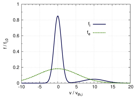
Figure 10.
Velocity distribution of ions (solid curve) and electrons (dotted curve) in a two-species plasma with a population of supra-thermal particles and equal bulk ion and electron temperatures. The ion/electron mass ratio is reduced to 30 for the sake of readability of the figure.
Based on quasi-linear theory, O’Neil demonstrated the existence of a kinetic subcritical instability of a spectrum of many modes [57]. This is due to the flattening in the velocity distribution, which effectively mitigates Landau damping. He argued that, in general, this subcritical instability is possible when the total resonant kinetic energy available for growth is less than the total resonant kinetic energy available for damping.
This theory discarded the role of nonlinear particle trapping, which was later found to be essential in many contexts, as discussed below. Here, by nonlinear particle trapping, we refer to the trapping of charged particles by their own electrostatic potential, which leads to a Bernstein-Greene-Kruskal (BGK)-like mode [58].
In many cases, a BGK vortex can evolve into a phase-space hole. A phase-space hole is a BGK-like structure with a local depression of phase-space density within the vortex. It can be seen as a kinetic counterpart of the fluid vortex. Although, in contrast to a fluid vortex, which lives in real (configuration) space, the phase-space hole lives in the phase-space of particle distribution, that is, real space and energy space. The existence of phase-space holes was predicted by numerical simulations of the two-beam instability [59], which were interpreted by theory [60,61] and experimentally observed in a wide variety of space and laboratory plasmas [62]. See the tutorial in Ref. [63] for a detailed description of phase-space structures or Refs. [64,65] for a review.
Dupree predicted analytically that phase-space holes can grow nonlinearly and drive subcritical instabilities [61,66].The mechanism is detailed in the next part, Section 4.2.2.
The theory of subcritical instabilities has been further developed in the conditions of Figure 10, but with an additional simplification of the model. In the Berk-Breizman model, the damping species is assumed to take only the role of a neutralizing background, and all damping processes are modeled by a linear external dissipation with a fixed rate [67]. In this system, subcritical instabilities have been observed in numerical simulations [68,69,70,71] and interpreted by analytical theory. Linear Landau damping generates a seed structure in phase-space that can grow nonlinearly as a result of dissipation acting as a drag force (see next section). The nonlinear growth rate was obtained based on a kinetic counterpart of the Charney–Drazin theorem on the non-acceleration of zonal mean flows by steady conservative waves [72]. The threshold of initial perturbation amplitude can be obtained by balancing the growth of a phase-space structure due to wave dissipation and its decay due to collisions. Figure 11 shows time-series of the electric field amplitude for different initial amplitudes, obtained by numerical simulation of the Berk–Breizman model. In all cases, dissipation is larger than linear drive, so the mode is linearly stable. The mode grows only if the initial amplitude is larger than a threshold, which is consistent with our nonlinear theory.
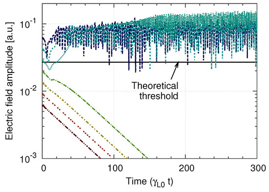
Figure 11.
Dashed curves: time-series of electric field amplitude for different initial amplitudes in a subcritical case (the dissipation/drive ratio is ). Solid line: theoretical nonlinear instability threshold [72].
In toroidal geometry, Kosuga et al. recently showed, by analytic calculations, the possibility of kinetic subcritical instabilities for the trapped ion mode [73]. They emphasized the destabilizing role of electron dissipation. Similarly to the 1D systems discussed above, the mechanism is based on the nonlinear growth of a hole structure in phase-space [61,74]. The mechanism still works in the present of turbulent decorrelation of such structures [75,76] so this is relevant to the context of granulation [77].
N’Guyen et al. investigated the situation of Figure 10 as well, but for a single sine wave [78]. They discussed another kind of subcritical instability that is driven by a nonlinear reduction of damping as well but is due to nonlinear particle trapping. Later, they showed that this type of subcritical instability is, in principle, relevant for acoustic modes, such as beta Alfvén eigenmodes or geodesic acoustic modes, under standard tokamak conditions [79].
Although these theories of kinetic subcritical instabilities predict essential impacts of subcritical instabilities on turbulence, transport, and mean flows, they do not yet provide any unambiguous macroscopic signature, which could help to discriminate these impacts from the similar impacts of linearly unstable modes. Moreover, there is no indication that the instability being subcritical is a key feature of the resulting turbulence, transport, and flows. In Section 4.3, we review the first experimental evidence of the strong effect of kinetic subcritical instability in a context where subcriticality does come with a key impact: abrupt growth. However, let us first detail the physical mechanism of nonlinear growth of a phase-space hole which is responsible for most of the kinetic subcritical instabilities.
4.2.2. Nonlinear Growth Mechanism of a Phase-Space Hole
Let us focus on a 1D plasma with ions and electrons, but unlike the situation of Figure 10, here, both ion and electron velocity distributions are Gaussian, and the electron distribution is shifted by a given mean velocity. Figure 12 shows the initial or equilibrium velocity distributions and as well as the distributions at some arbitrary time in the presence of a single electron hole. The electron hole can grow nonlinearly in this situation, where in the vicinity of the hole, the electron velocity gradient is positive and the ion velocity gradient is negative. The impact of the electron hole on the ion distribution is represented as a barely visible flattening. Figure 13 is a cartoon of the electron hole in phase-space. Trapped electrons form a vortex structure with a deficit of phase-space density (in other words, a negative perturbation of the distribution function, ). Therefore the electron density features a local deficit as well, which is consistent with the local bump of potential, which, in turn, is consistent with the trapping of electrons. Therefore, the BGK-like vortex forms a self-consistent, self-sustained (in the absence of collisions) structure. Here, to simplify the discussion, the perturbation in the ion density is assumed to be negligible.
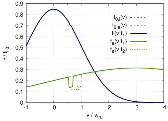
Figure 12.
Velocity distribution of ions and electrons in a two-species plasma with a mean velocity drift. The equilibrium distributions are noted and . The ion/electron mass ratio is reduced to 10 for the sake of readability of the figure. An electron hole is drawn schematically at some arbitrary time , and the mechanism of its growth from to a later time is explained in the text as the result of a drag force due to the scattering of ions by the electron hole.
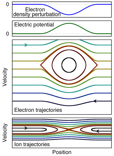
Figure 13.
Cartoon of an electron hole in the reference frame of the hole. From top to bottom: electron density perturbation, electric potential, electron trajectories, and ion trajectories. Here, the scales are consistent with a mass ratio .
The nonlinear mechanism of growth of this electron hole can be understood based on the latter figures, Figure 12 and Figure 13.
Firstly, if the hole changes its mean velocity slowly enough, trapped electrons within the hole will move along with the hole. Detrapping is rare enough for slow changes in the velocity of the hole. Since the Vlasov equation states that the distribution function f is conserved along particle orbits, the value of f at the bottom of the hole will remain constant even as the hole accelerates or decelerates. Therefore, since the equilibrium electron distribution has a positive slope in the vicinity of the hole, the hole deepens if its mean velocity increases, as schematized in Figure 12.
Secondly, in this configuration, there is a force that does accelerate the hole, leading to its growth. Here, the impact of electron hole on ions is essential. The ion trajectories are shown in the bottom of Figure 13. The positive charge of the electron hole scatters ions in both directions away from the center of the hole. Due to the negative gradient of the ion velocity distribution, there is an imbalance between decelerated ions and accelerated ions—ions, as a whole, gain momentum. Electrons, on the contrary, lose momentum (ensuring total momentum conservation). The result for the electron hole, which has a negative mass, is to accelerate.
Let us give a rough estimate of the nonlinear growth rate by noting u as the velocity of the hole, h as the hole depth (), as the width of the hole, as the amplitude of the trapping potential, and as the equilibrium velocity gradient for species s in the vicinity of the hole. A simple calculation of particle orbits yields that is proportional to . The positive charge of the electron hole scatters ions, which, because of the negative gradient of , leads to a positive force on ions. proportional to . The equal and opposite reaction is a drag force on electrons, . As a result, the electron hole accelerates at a rate of , where is the negative mass of the hole which is proportional to . Since the trapped-electron distribution function remains constant, the hole deepens at a rate of proportional to . Finally, Poisson equation shows that is roughly proportional to ; therefore, h is proportional to . Putting the above relations of proportionality together, we obtain a growth rate proportional to .
The full calculation is tedious and takes into account additional effects such as potential screening and the retroaction of the growth on the drag force [66,80]. However, the final result is consistent with the above simplified mechanism.
This nonlinear growth of phase-space holes was confirmed by Berman et al. in numerical simulations of the ion-acoustic instability in 1D collisionless electron–ion plasmas with a velocity drift (but no supra-thermal population) [81]. They performed Lagrangian (particle-in-cell) simulations with an initial sine perturbation. They found that a subcritical instability with a very small threshold in amplitude was developing, even for velocity drifts much below the linear threshold. Recently, we found, by both Lagrangian and semi-Lagrangian simulations, that these results are attributable to the spurious numerical noise due to the low number of particles that could reasonably be calculated given the computing resources of the 1980s [82]. However, with modern computing [83], we still obtained unambiguous subcritical instabilities, given an initial sine perturbation with large initial amplitude (), or, more importantly, given an initial BGK-like perturbation even with a small initial amplitude ().
For the origin of a large-enough initial perturbation or initial BGK-like fluctuations, we have discussed three plausible scenarios [82]. The first scenario is a growth from, e.g., thermal fluctuations, which is limited to an initial barely stable equilibrium. The second scenario is the growth of a hole that would have been externally driven by the experimental setup or convected from a region of linear instability. The third scenario is the case of self-sustained turbulence, as plasma conditions go from linearly unstable to subcritical on a slow time-scale.
4.3. Hybrid Fluid-Kinetic Subcritical Instabilities
Despite decades of theoretical advances, experimental observations of kinetic subcritical instabilities have been lacking, probably in part because it is difficult to measure the velocity-space distribution in relevant conditions. However, recently, a good candidate was identified experimentally [84] and interpreted by theory as a subcritical instability driven by a combination of fluid and kinetic nonlinearities [85].
In the helical plasma of the Large Helical Device (LHD), bursts of geodesic acoustic mode driven by energetic particles (EGAM) are sometimes accompanied by a much more abrupt, large-amplitude burst of another mode. The observation cannot be explained by conventional mechanisms, such as nonlinear coupling of turbulence alone [86], or resonant interaction with energetic particles [87]. In particular, the measurements point to a threshold in amplitude of the EGAM for the destabilization of the abrupt mode.
We proposed a theoretical interpretation based on a reduced 1D model, including both fluid and kinetic nonlinearities [85]. The model qualitatively recovers the experimental observations in terms of temporal evolution and phase relation with the input parameters being consistent with the measured plasma parameters. Within the framework of this model, we found that the abrupt burst belongs to a new class of subcritical instability which is a hybrid between fluid and kinetic subcritical instabilities. In fact, we found two distinct regimes, depending mainly on collisionality [88]. For very low collisionality, nonlinear fluid coupling between modes provides a seed perturbation, which evolves due to particle trapping into a phase-space hole, and then grows, dominated by kinetic nonlinearity. In contrast, for slightly higher collisionality, the subcritical instability requires both fluid and kinetic nonlinearities to continuously collaborate. The LHD observation was interpreted as a manifestation of the latter one.
In this context, it is the fact that the instability is subcritical which yields such abrupt growth with a growth-rate of one order-of-magnitude above that of its supercritical counterpart.
5. Conclusions
Subcritical instabilities are ubiquitous in neutral fluids and in plasmas and merit attention since the access to free energy and the spectrum of turbulence are ultimately nonlinear issues. Subcritical instabilities have common characteristics, such as a threshold in amplitude and a growth rate that increases with increasing amplitude. However, they can originate from a wide variety of physical mechanisms.
In plasmas, subcritical instabilities are of great interest due to their essential impact on the onset of turbulence [89,90], structure formation [91], anomalous resistivity [82,92], and potentially, turbulent transport [73].
To widen the scope, we invite the interested reader to look into the literature on subcritical instabilities in other areas that we have not discussed in this paper. Let us give a non-exhaustive list of examples: (1) the follower-loaded double pendulum in vibrational mechanics [93], (2) the dynamics of railway vehicles [94], (3) acoustic waves [95] and flame dynamics [96] in combustion chambers, (4) spin-waves in magnetic nanocontact systems [97], and (5) the zigzag transition for confined repelling particles in quasi-1D chemical physics [98,99].
Author Contributions
Writing—original draft, M.L.; Writing—review & editing, J.M., M.S. and A.S.
Funding
This work was carried out within the framework of the EUROfusion consortium and the French Research Federation for Fusion Studies. The views and opinions expressed herein do not necessarily reflect those of the European Commission.
Acknowledgments
Maxime Lesur is grateful for stimulating discussions with the participants in the Festival de Théorie.
Conflicts of Interest
The authors declare no conflict of interest.
References
- Dauchot, O.; Manneville, M. Local Versus Global Concepts in Hydrodynamic Stability Theory. J. Phys. II Fr. 1997, 7, 371–389. [Google Scholar] [CrossRef]
- Yoshizawa, A.; Itoh, S.; Itoh, K. Plasma and Fluid Turbulence: Theory and Modelling; Series in Plasma Physics and Fluid Dynamics; CRC Press: Boca Raton, FL, USA, 2002. [Google Scholar]
- Schmid, P.J. Nonmodal stability theory. Annu. Rev. Fluid Mech. 2007, 39, 129–162. [Google Scholar] [CrossRef]
- Lesur, M.; Sasaki, M.; Shimizu, A. Subcritical Instabilities in Neutral Fluids and Plasmas. J. Plasma Fusion Res. 2016, 92, 665–671. [Google Scholar]
- Chanson, H. Physical Modelling of Hydraulics. In The Hydraulics of Open Channel Flow: An Introduction; Butterworth-Heinemann: Oxford, UK, 1999. [Google Scholar]
- Couette, M. Etudes sur le Frottement des Liquides. Ph.D. Thesis, Faculté des Sciences, Paris, France, 1890. [Google Scholar]
- Davies, S.; White, C. An experimental study of the flow of water in pipes of rectangular section. Proc. R. Soc. Lond. A 1928, 119, 92–107. [Google Scholar] [CrossRef]
- Coles, D. Transition in circular Couette flow. J. Fluid Mech. 1965, 21, 385–425. [Google Scholar] [CrossRef]
- Tillmark, N.; Alfredsson, P.H. Experiments on transition in plane Couette flow. J. Fluid Mech. 1992, 235, 89–102. [Google Scholar] [CrossRef]
- Lundbladh, A.; Johansson, A.V. Direct simulation of turbulent spots in plane Couette flow. J. Fluid Mech. 1991, 229, 499–516. [Google Scholar] [CrossRef]
- Trefethen, L.N.; Trefethen, A.E.; Reddy, S.C.; Driscoll, T.A. Hydrodynamic stability without eigenvalues. Science 1993, 261, 578–584. [Google Scholar] [CrossRef] [PubMed]
- Drazin, P.; Reid, W. Hydrodynamic Stability; Cambridge University Press: Cambridge, UK, 1981. [Google Scholar]
- Grossmann, S. The onset of shear flow turbulence. Rev. Mod. Phys. 2000, 72, 603. [Google Scholar] [CrossRef]
- Manneville, P. On the transition to turbulence of wall-bounded flows in general, and plane Couette flow in particular. Eur. J. Mech.-B 2015, 49, 345–362. [Google Scholar] [CrossRef]
- Borrero, D. Subcritical Transition to Turbulence in Taylor-Couette Flow. Ph.D. Thesis, Georgia Institute of Technology, Atlanta, GA, USA, 2014. [Google Scholar]
- Meignin, L.; Gondret, P.; Ruyer-Quil, C.; Rabaud, M. Subcritical Kelvin-Helmholtz Instability in a Hele-Shaw Cell. Phys. Rev. Lett. 2003, 90, 234502. [Google Scholar] [CrossRef] [PubMed]
- Groisman, A.; Steinberg, V. Mechanism of elastic instability in Couette flow of polymer solutions: Experiment. Phys. Fluids 1998, 10, 2451–2463. [Google Scholar] [CrossRef]
- Morozov, A.N.; van Saarloos, W. An introductory essay on subcritical instabilities and the transition to turbulence in visco-elastic parallel shear flows. Phys. Rev. 2007, 447, 112–143. [Google Scholar] [CrossRef]
- Manneville, P. Instabilités, Chaos et Turbulence; Editions de l’Ecole Polytechnique: Palaiseau, France, 2004. [Google Scholar]
- Weissman, M.A. Nonlinear Wave Packets in the Kelvin-Helmholtz Instability. Philos. Trans. R. Soc. Lond. A 1979, 290, 639–681. [Google Scholar] [CrossRef]
- Kühnen, J.; Braunshier, P.; Schwegel, M.; Kuhlmann, H.; Hof, B. Subcritical versus supercritical transition to turbulence in curved pipes. J. Fluid Mech. 2015, 770. [Google Scholar] [CrossRef]
- Henningson, D.S.; Alfredsson, P.H. The wave structure of turbulent spots in plane Poiseuille flow. J. Fluid Mech. 1987, 178, 405–421. [Google Scholar] [CrossRef]
- Gad-El-Hak, M.; Blackwelderf, R.F.; Riley, J.J. On the growth of turbulent regions in laminar boundary layers. J. Fluid Mech. 1981, 110, 73–95. [Google Scholar] [CrossRef]
- Klingmann, B.G.B.; Alfredsson, P.H. Turbulent spots in plane Poiseuille flow—Measurements of the velocity field. Phys. Fluids A 1990, 2, 2183–2195. [Google Scholar] [CrossRef]
- Dauchot, O.; Daviaud, F. Finite amplitude perturbation and spots growth mechanism in plane Couette flow. Phys. Fluids 1995, 7, 335–343. [Google Scholar] [CrossRef]
- Sengupta, T.; Lim, T.; Chattopadhyay, M. An Experimental and Theoretical Investigation of a By-Pass Transition Mechanism; Technical Report, IITK/Aero/AD/2001/02; I.I.T. Kanpur: Kanpur, India, 2001. [Google Scholar]
- Sengupta, T.K.; De, S.; Sarkar, S. Vortex-induced instability of an incompressible wall-bounded shear layer. J. Fluid Mech. 2003, 493, 277–286. [Google Scholar] [CrossRef]
- Lim, T.; Sengupta, T.; Chattopadhyay, M. A visual study of vortex-induced subcritical instability on a flat plate laminar boundary layer. Exp. Fluids 2004, 37, 47–55. [Google Scholar] [CrossRef]
- Henningson, D.S.; Lundbladh, A.; Johansson, A.V. A mechanism for bypass transition from localized disturbances in wall-bounded shear flows. J. Fluid Mech. 1993, 250, 169–207. [Google Scholar] [CrossRef]
- Manneville, P. Understanding the sub-critical transition to turbulence in wall flows. Pramana 2008, 70, 1009–1021. [Google Scholar] [CrossRef]
- Waleffe, F. On a self-sustaining process in shear flows. Phys. Fluids 1997, 9, 883–900. [Google Scholar] [CrossRef]
- Waleffe, F.; Wang, J. Transition threshold and the self-sustaining process. In IUTAM Symposium on Laminar-Turbulent Transition and Finite Amplitude Solutions; Springer: Berlin, Germany, 2005; pp. 85–106. [Google Scholar]
- Faisst, H.; Eckhardt, B. Traveling waves in pipe flow. Phys. Rev. Lett. 2003, 91, 224502. [Google Scholar] [CrossRef] [PubMed]
- Wedin, H.; Kerswell, R.R. Exact coherent structures in pipe flow: Travelling wave solutions. J. Fluid Mech. 2004, 508, 333–371. [Google Scholar] [CrossRef]
- Hof, B.; van Doorne, C.W.; Westerweel, J.; Nieuwstadt, F.T.; Faisst, H.; Eckhardt, B.; Wedin, H.; Kerswell, R.R.; Waleffe, F. Experimental observation of nonlinear traveling waves in turbulent pipe flow. Science 2004, 305, 1594–1598. [Google Scholar] [CrossRef] [PubMed]
- Pomeau, Y. Front motion, metastability and subcritical bifurcations in hydrodynamics. Physica D 1986, 23, 3. [Google Scholar] [CrossRef]
- Shrira, V.; Voronovich, V.; Kozhelupova, N. Explosive instability of vorticity waves. J. Phys. Oceanogr. 1997, 27, 542–554. [Google Scholar] [CrossRef]
- Dodd, N.; Iranzo, V.; Caballería, M. A subcritical instability of wave-driven alongshore currents. J. Geophys. Res. Oceans 2004, 109. [Google Scholar] [CrossRef]
- Biskamp, D.; Walter, M. Suppression of shear damping in drift wave turbulence. Phys. Lett. A 1985, 109, 34–38. [Google Scholar] [CrossRef]
- Scott, B.D. Self-sustained collisional drift-wave turbulence in a sheared magnetic field. Phys. Rev. Lett. 1990, 65, 3289–3292. [Google Scholar] [CrossRef] [PubMed]
- Drake, J.F.; Zeiler, A.; Biskamp, D. Nonlinear Self-Sustained Drift-Wave Turbulence. Phys. Rev. Lett. 1995, 75, 4222–4225. [Google Scholar] [CrossRef] [PubMed]
- Baver, D.; Terry, P.; Fernandez, E. Nonlinear instability driven by advection of electron density in collisionless plasmas. Phys. Lett. A 2000, 267, 188–193. [Google Scholar] [CrossRef]
- Terry, P.; Baver, D.; Gupta, S. Role of stable eigenmodes in saturated local plasma turbulence. Phys. Plasmas 2006, 13, 022307. [Google Scholar] [CrossRef]
- Highcock, E.; Barnes, M.; Schekochihin, A.; Parra, F.; Roach, C.; Cowley, S. Transport bifurcation in a rotating tokamak plasma. Phys. Rev. Lett. 2010, 105, 215003. [Google Scholar] [CrossRef] [PubMed]
- Highcock, E.; Barnes, M.; Parra, F.; Schekochihin, A.; Roach, C.; Cowley, S. Transport bifurcation induced by sheared toroidal flow in tokamak plasmas. Phys. Plasmas 2011, 18, 102304. [Google Scholar] [CrossRef]
- Highcock, E.; Schekochihin, A.; Cowley, S.; Barnes, M.; Parra, F.; Roach, C.; Dorland, W. Zero-turbulence manifold in a toroidal plasma. Phys. Rev. Lett. 2012, 109, 265001. [Google Scholar] [CrossRef] [PubMed]
- Van Wyk, F.; Highcock, E.; Schekochihin, A.; Roach, C.; Field, A.; Dorland, W. Transition to subcritical turbulence in a tokamak plasma. J. Plasma Phys. 2016, 82. [Google Scholar] [CrossRef]
- van Wyk, F.; Highcock, E.; Field, A.; Roach, C.; Schekochihin, A.; Parra, F.; Dorland, W. Ion-scale turbulence in MAST: Anomalous transport, subcritical transitions, and comparison to BES measurements. Plasma Phys. Control. Fusion 2017, 59, 114003. [Google Scholar] [CrossRef]
- Yagi, M.; Itoh, S.; Itoh, K.; Fukuyama, A.; Azumi, M. Self-sustained plasma turbulence due to current diffusion. Phys. Plasmas 1995, 2, 4140–4148. [Google Scholar] [CrossRef]
- Itoh, K.; Itoh, S.I.; Fukuyama, A. Theory of anomalous transport in high-aspect-ratio toroidal helical plasmas. Phys. Rev. Lett. 1992, 69, 1050–1053. [Google Scholar] [CrossRef] [PubMed]
- Itoh, K.; Itoh, S.I.; Yagi, M.; Fukuyama, A. Subcritical Excitation of Plasma Turbulence. J. Phys. Soc. Jpn. 1996, 65, 2749–2752. [Google Scholar] [CrossRef]
- Carrera, R.; Hazeltine, R.D.; Kotschenreuther, M. Island bootstrap current modification of the nonlinear dynamics of the tearing mode. Phys. Fluids 1986, 29, 899–902. [Google Scholar] [CrossRef]
- Johnson, B.M.; Gammie, C.F. Linear theory of thin, radially stratified disks. Astr. J. 2005, 626, 978. [Google Scholar] [CrossRef]
- Friedman, B.; Carter, T. A non-modal analytical method to predict turbulent properties applied to the Hasegawa-Wakatani model. Phys. Plasmas 2015, 22, 012307. [Google Scholar] [CrossRef]
- Pringle, C.C.; McMillan, B.F.; Teaca, B. A nonlinear approach to transition in subcritical plasmas with sheared flow. Phys. Plasmas 2017, 24, 122307. [Google Scholar] [CrossRef]
- McMillan, B.F.; Pringle, C.C.; Teaca, B. Simple advecting structures and the edge of chaos in subcritical tokamak plasmas. arXiv, 2018; arXiv:1802.08519. [Google Scholar]
- O’Neil, T.M. Nonlinear Instability. Phys. Fluids 1967, 10, 1027–1030. [Google Scholar] [CrossRef]
- Bernstein, I.; Greene, J.; Kruskal, M.D. Exact nonlinear plasma oscillations. Phys. Rev. 1957, 108, 546–550. [Google Scholar] [CrossRef]
- Roberts, K.V.; Berk, H.L. Nonlinear Evolution of a Two-Stream Instability. Phys. Rev. Lett. 1967, 19, 297–300. [Google Scholar] [CrossRef]
- Schamel, H. Theory of Electron Holes. Phys. Scr. 1979, 20, 336. [Google Scholar] [CrossRef]
- Dupree, T.H. Theory of phase-space density holes. Phys. Fluids 1982, 25, 277–289. [Google Scholar] [CrossRef]
- Eliasson, B.; Shukla, P. Formation and dynamics of coherent structures involving phase-space vortices in plasmas. Phys. Rep. 2006, 422, 225–290. [Google Scholar] [CrossRef]
- Kosuga, Y.; Lesur, M. Development of Plasma Turbulence Research into Phase Space. J. Plasma Fusion Res. 2014, 90, 289–295. [Google Scholar]
- Luque, A.; Schamel, H. Electrostatic trapping as a key to the dynamics of plasmas, fluids and other collective systems. Phys. Rep. 2005, 415, 261–359. [Google Scholar] [CrossRef]
- Schamel, H. Cnoidal electron hole propagation: Trapping, the forgotten nonlinearity in plasma and fluid dynamics. Phys. Plasmas 2012, 19, 020501. [Google Scholar] [CrossRef]
- Dupree, T.H. Growth of phase-space density holes. Phys. Fluids 1983, 26, 2460–2481. [Google Scholar] [CrossRef]
- Berk, H.L.; Breizman, B.N. Saturation of a single mode driven by an energetic injected beam. I. Plasma wave problem. Phys. Fluids B 1990, 2, 2226–2234. [Google Scholar] [CrossRef]
- Berk, H.L.; Breizman, B.N.; Candy, J.; Pekker, M.; Petviashvili, N.V. Spontaneous hole-clump pair creation. Phys. Plasmas 1999, 6, 3102–3113. [Google Scholar] [CrossRef]
- Lesur, M.; Idomura, Y.; Garbet, X. Fully nonlinear features of the energetic beam-driven instability. Phys. Plasmas 2009, 16, 092305. [Google Scholar] [CrossRef]
- Lesur, M.; Idomura, Y.; Shinohara, K.; Garbet, X.; the JT-60 Team. Spectroscopic determination of kinetic parameters for frequency sweeping Alfvén eigenmodes. Phys. Plasmas 2010, 17, 122311. [Google Scholar] [CrossRef]
- Lesur, M.; Idomura, Y. Nonlinear categorization of the energetic-beam-driven instability with drag and diffusion. Nucl. Fusion 2012, 52, 094004. [Google Scholar] [CrossRef]
- Lesur, M.; Diamond, P.H. Nonlinear instabilities driven by coherent phase-space structures. Phys. Rev. E 2013, 87, 031101. [Google Scholar] [CrossRef]
- Kosuga, Y.; Itoh, S.I.; Diamond, P.; Itoh, K.; Lesur, M. Role of phase space structures in collisionless drift wave turbulence and impact on transport modeling. Nucl. Fusion 2017, 57, 072006. [Google Scholar] [CrossRef]
- Terry, P.W.; Diamond, P.H.; Hahm, T.S. The structure and dynamics of electrostatic and magnetostatic drift holes. Phys. Fluids B 1990, 2, 2048–2063. [Google Scholar] [CrossRef]
- Biglari, H.; Diamond, P.H.; Terry, P.W. Theory of trapped-ion temperature-gradient-driven turbulence and transport in low-collisionality plasmas. Phys. Fluids 1988, 31, 2644–2658. [Google Scholar] [CrossRef]
- Kosuga, Y.; Itoh, S.I.; Diamond, P.H.; Itoh, K.; Lesur, M. Ion temperature gradient driven turbulence with strong trapped ion resonance. Phys. Plasmas 2014, 21, 102303. [Google Scholar] [CrossRef]
- Dupree, T.H. Theory of Phase Space Density Granulation in Plasma. Phys. Fluids 1972, 15, 334–344. [Google Scholar] [CrossRef]
- Nguyen, C.; Lütjens, H.; Garbet, X.; Grandgirard, V.; Lesur, M. Existence of metastable kinetic modes. Phys. Rev. Lett. 2010, 105, 205002. [Google Scholar] [CrossRef] [PubMed]
- Nguyen, C.; Garbet, X.; Grandgirard, V.; Decker, J.; Guimarães-Filho, Z.; Lesur, M.; Lütjens, H.; Merle, A.; Sabot, R. Nonlinear modification of the stability of fast particle driven modes in tokamaks. Plasma Phys. Control. Fusion 2010, 52, 124034. [Google Scholar] [CrossRef]
- Tetreault, D.J. Growth rate of the clump instability. Phys. Fluids 1983, 26, 3247–3261. [Google Scholar] [CrossRef]
- Berman, R.H.; Tetreault, D.J.; Dupree, T.H.; Boutros-Ghali, T. Computer Simulation of Nonlinear Ion-Electron Instability. Phys. Rev. Lett. 1982, 48, 1249–1252. [Google Scholar] [CrossRef]
- Lesur, M.; Diamond, P.H.; Kosuga, Y. Nonlinear current-driven ion-acoustic instability driven by phase-space structures. Plasma Phys. Control. Fusion 2014, 56, 075005. [Google Scholar] [CrossRef]
- Lesur, M. Method- and scheme-independent entropy production in turbulent kinetic simulations. Comput. Phys. Commun. 2016, 200, 182–189. [Google Scholar] [CrossRef]
- Ido, T.; Itoh, K.; Osakabe, M.; Lesur, M.; Shimizu, A.; Ogawa, K.; Toi, K.; Nishiura, M.; Kato, S.; Sasaki, M.; et al. Strong Destabilization of Stable Modes with a Half-Frequency Associated with Chirping Geodesic Acoustic Modes in the Large Helical Device. Phys. Rev. Lett. 2016, 116, 015002. [Google Scholar] [CrossRef] [PubMed]
- Lesur, M.; Itoh, K.; Ido, T.; Osakabe, M.; Ogawa, K.; Shimizu, A.; Sasaki, M.; Ida, K.; Inagaki, S.; Itoh, S.I.; et al. Nonlinear Excitation of Subcritical Instabilities in a Toroidal Plasma. Phys. Rev. Lett. 2016, 116, 015003. [Google Scholar] [CrossRef] [PubMed]
- Diamond, P.H.; Itoh, S.I.; Itoh, K.; Hahm, T.S. Zonal flows in plasma—A review. Plasma Phys. Control. Fusion 2005, 47, R35. [Google Scholar] [CrossRef]
- Fu, G.Y. Energetic-Particle-Induced Geodesic Acoustic Mode. Phys. Rev. Lett. 2008, 101, 185002. [Google Scholar] [CrossRef] [PubMed]
- Lesur, M.; Itoh, K.; Ido, T.; Itoh, S.I.; Kosuga, Y.; Sasaki, M.; Inagaki, S.; Osakabe, M.; Ogawa, K.; Shimizu, A.; et al. Nonlinear excitation of subcritical fast ion-driven modes. Nucl. Fusion 2016, 56, 056009. [Google Scholar] [CrossRef]
- Landau, L. On the vibrations of the electronic plasma. J. Phys. 1946, 10, 25–34. [Google Scholar]
- Itoh, K.; Itoh, S.I.; Kosuga, Y.; Lesur, M.; Ido, T. Onset condition of the subcritical geodesic acoustic mode instability in the presence of energetic-particle-driven geodesic acoustic mode. Plasma Phys. Rep. 2016, 42, 418–423. [Google Scholar] [CrossRef]
- Cross, M.C.; Hohenberg, P.C. Pattern formation outside of equilibrium. Rev. Mod. Phys. 1993, 65, 851–1112. [Google Scholar] [CrossRef]
- Lesur, M.; Diamond, P.H.; Kosuga, Y. Phase-space jets drive transport and anomalous resistivity. Phys. Plasmas 2014, 21. [Google Scholar] [CrossRef]
- Iliya, B. Selected Topics in Vibrational Mechanics; World Scientific: Singapore, 2004; Volume 11. [Google Scholar]
- Xue-jun, G.; True, H.; Li, Y. Lateral dynamic features of a railway vehicle. Proc. Inst. Mech. Eng. Part F J. Rail Rapid Transit 2015, 230. [Google Scholar] [CrossRef]
- Ananthkrishnan, N.; Deo, S.; Culick, F. Modeling and Dynamics of Nonlinear Acoustic Waves in a Combustion Chamber. Combust. Sci. Technol. 2005, 177. [Google Scholar] [CrossRef]
- Ebi, D.; Denisov, A.; Bonciolini, G.; Boujo, E.; Noiray, N. Flame Dynamics Intermittency in the Bistable Region Near a Subcritical Hopf Bifurcation. J. Eng. Gas Turbines Power 2018, 140, 061504. [Google Scholar] [CrossRef]
- Consolo, G.; Finocchio, G.; Lopez-Diaz, L.; Azzerboni, B. Numerical analysis of the nonlinear excitation of subcritical spin-wave modes within a micromagnetic framework. IEEE Trans. Magn. 2009, 45, 5220–5223. [Google Scholar] [CrossRef]
- Straube, A.V.; Dullens, R.P.; Schimansky-Geier, L.; Louis, A.A. Zigzag transitions and nonequilibrium pattern formation in colloidal chains. J. Chem. Phys. 2013, 139, 134908. [Google Scholar] [CrossRef] [PubMed]
- Dessup, T.; Coste, C.; Saint Jean, M. Subcriticality of the zigzag transition: A nonlinear bifurcation analysis. Phys. Rev. E 2015, 91, 032917. [Google Scholar] [CrossRef] [PubMed]


© 2018 by the authors. Licensee MDPI, Basel, Switzerland. This article is an open access article distributed under the terms and conditions of the Creative Commons Attribution (CC BY) license (http://creativecommons.org/licenses/by/4.0/).