Article

Derivation of the Variants of the Burgers Model Using a Thermodynamic Approach and Appealing to the Concept of Evolving Natural Configurations

1
Faculty of Mathematics and Physics, Charles University, Sokolovská 83, Praha 8, CZ 186 75, Czech Republic
2
Department of Mechanical Engineering, Texas A&M University, College Station, TX 77843, USA
*
Author to whom correspondence should be addressed.
Fluids 2018, 3(4), 69; https://doi.org/10.3390/fluids3040069
Submission received: 3 September 2018 / Revised: 22 September 2018 / Accepted: 24 September 2018 / Published: 26 September 2018

Abstract

:
Viscoelastic rate-type fluid models involving the stress and frame-indifferent time derivatives of second order, like those in Burgers’ model, are used to describe the complicated response of fluid like materials that are endowed with a complex microstructure that allows them to possess two different relaxation mechanisms as well as other non-Newtonian characteristics. Such models are used in geomechanics, biomechanics, chemical engineering and material sciences. We show how to develop such rate-type fluid models that include the classical Burgers’ model as well as variants of Burgers’ model, using a thermodynamic approach based on constitutive assumptions for two scalar quantities (namely, how the material stores energy and how the energy is dissipated) and appealing to the concept of natural configuration associated with the placement of the body that evolves as the body deforms.

1. Introduction

To describe non-Newtonian phenomena such as stress relaxation, nonlinear creep and normal stress differences exhibited by geomaterials like asphalt or biomaterials like the vitreous in the eye, rate-type viscoelastic fluid models are commonly used. These materials exhibit more than one relaxation mechanism (see Narayan et al. [1], Sharif-Kashani et al. [2]) that can be identified by the different relaxation times observed in experimental studies. The presence of more than one relaxation time excludes the classical Maxwell model (originally proposed by Maxwell [3] in one spatial dimension) or the Oldroyd-B model (see Oldroyd [4] who developed the first general systematic three-dimensional theory to develop proper frame indifferent rate-type viscoelastic models) from one’s consideration. On the other hand, the presence of multiple relaxation times in the response of materials in creep or stress relaxation tests can be well described by rate-type fluid models of higher order. An example of a higher order model capable of describing two different relaxation times is the model due to Burgers. In the case of asphalt, Monismith and Secor [5], Narayan et al. [1] and Málek et al. [6] used the model due to Burgers to corroborate experimental data, while in the case of the vitreous of the bovine eye, Sharif-Kashani et al. [2] correlated experimental data also using a Burgers model.
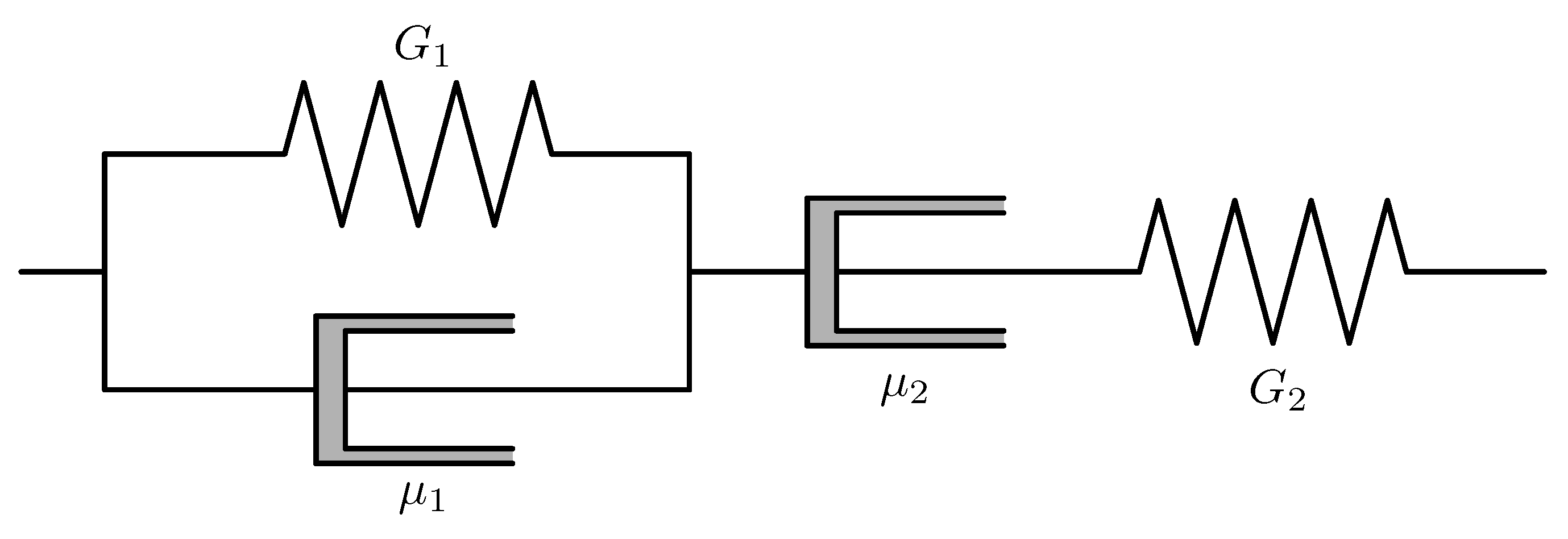
The model proposed by Burgers [7] in one spatial dimension can be associated with as many as four different mechanical systems consisting of springs and dashpots. The Maxwell fluid model and the Kelvin–Voigt solid model are special cases of the Burgers model (see Figure 1).
The relation between the stress σ and the strain ε for this one-dimensional model satisfies the second order differential equation
σ + λ 1 σ ˙ + λ 2 σ ¨ = η 1 ε ˙ + η 2 ε ¨ ,
where the constant parameters λ 1 , λ 2 , η 1 , η 2 can be expressed in the terms of the shear moduli G 1 , G 2 and the viscosities μ 1 , μ 2 
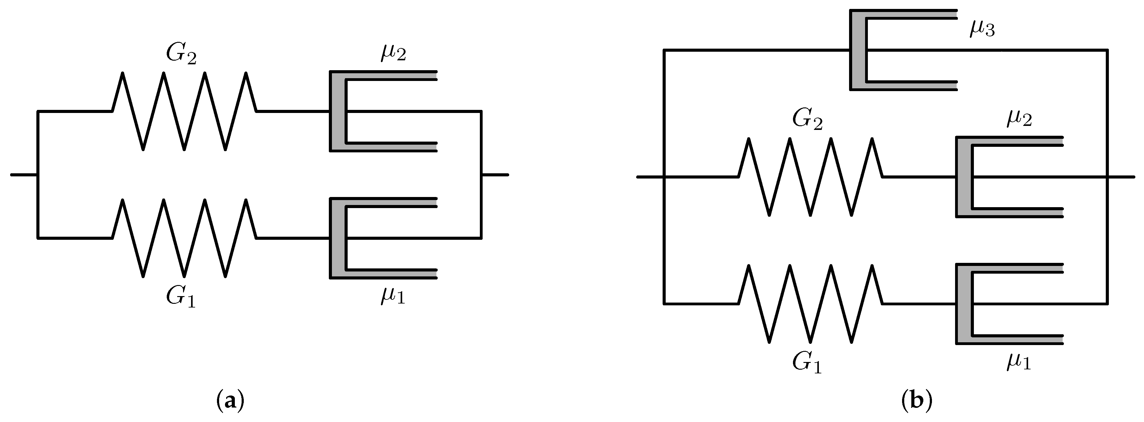
. We can also consider a system of two Maxwell elements in parallel, see Figure 2a, that gives the same constitutive relation as in (1).
Since many materials possess some additional viscous dissipation (connected, for example, with the properties of an aqueous plasma), it is desirable to add an additional dashpot in parallel (see Figure 2b). A possible generalization of the setting sketched in Figure 2b to three dimensions reads as
T = p I + 2 μ D + S , S + G 1 μ 1 + G 2 μ 2 S + G 1 G 2 μ 1 μ 2 S = 2 G 1 G 2 1 μ 1 + 1 μ 2 D + 2 ( G 1 + G 2 ) D ,
where T is the Cauchy stress, I is the identity tensor, and p is a scalar associated with the fact that the fluid is incompressible (Note that p is merely the indeterminate part of the stress and the symbol gives the impression that it is the pressure, a term that is ill-understood, see [8]. We continue to use the symbol p as it is a conventional notation.). The symbol S = t + ( v · ) ( v ) ( v ) T denotes the upper convected Oldroyd derivative, v is the velocity and D is the symmetric part of velocity gradient (see the definitions of the kinematical quantities introduced in the next section). There are however subtle issues connected with these constitutive equations. First, a generalization from one-dimensional mechanical analog to three-dimensional model is not unique and, in principle, other objective derivatives such as the Jaumann–Zaremba or Gordon–Schowalter can be used instead of the upper convected Oldroyd derivative. Second, it is not at all obvious that generalizations of the form (2) satisfy the second law of thermodynamics.
In order to overcome these issues, Rajagopal and Srinivasa [9] proposed a methodology to derive thermodynamically consistent viscoelastic rate-type fluid models. Their derivation is based on the notion that as the body produces entropy the natural configuration associated with the body evolves. The existence of a natural configuration that evolves as a body deforms allows one to split the total deformation into that associated with the purely elastic response and the dissipative response. Then by prescribing two constitutive relations for two scalar quantities: the Helmholtz free energy ψ (or the Gibbs potential) describing the elastic response of the body and the rate of entropy production ξ that characterizes how the body dissipates energy, they obtained the form of the Cauchy stress tensor T including its evolution equation. Later, this approach was used to obtain a generalization of Burgers’ model (Rajagopal and Srinivasa [10], Krishnan and Rajagopal [11], Krishnan and Rajagopal [12], Karra and Rajagopal [13], Málek et al. [14]). A new idea that is used in these studies is to connect two different relaxation times with two different underlying natural configurations. Even though the complex models that are obtained do not exactly coincide with the model (2), it was shown that when the elastic response between the natural configuration and the current configuration is linearized, then all these models reduce to the model (2). This may, at first glance, indicate that the classical Burgers model is an approximation rather than a proper model in its own right.
The first purpose of this study is to show that model (2) can be obtained directly without any additional linearization or through a reduction of more complex models. In this regard, we follow a recent study Málek et al. [15] where we show how to derive the classical Maxwell and Oldroyd-B model using the thermodynamic approach based on the notion of natural configuration. The basic step that makes the analysis possible is the following. The standard models due to Maxwell, Oldroyd and Burgers usually concern incompressible materials. It means that all admissible deformations have to be isochoric. Since the introduction of the notion of natural configuration allows one to split any process into an elastic response from an evolving natural configuration and a dissipative process describing (irreversible) changes in the natural configuration, it seems reasonable to require that, if the total process is isochoric, then its instantaneous elastic part is isochoric as well. However, Málek et al. [6] found that, if they gave up the requirement that both the elastic and dissipative responses be isochoric and only required that the compound response be isochoric, then they were able to develop the Maxwell and Oldroyd-B model without resorting to any approximation. We refer the reader to [15] for a detailed discussion of this issue. Following [15], we will require, in this study, that the total deformation process is isochoric while its instantaneous elastic part and its purely dissipative part are not necessarily isochoric.
The constitutive assumptions for the Helmholtz energy ψ and the rate of entropy production ξ provide, in a straightforward way, a priori energy estimates (see for example [16,17]), lead to the correct and complete form of the evolution equation for temperature ([18]) and automatically guarantee the stability of the rest state. Furthermore, the knowledge of the Lyapunov functional connected with such complex systems helps one to construct a distance measure that can be used in studying the stability of the steady states, error between two solutions (regular and weak one, discrete and continuous), etc. (see [19,20,21,22]).
The generalized Burgers models are obtained using two natural configurations, which yields a set of two first order differential equations for the parts of the Cauchy stress tensor. This immediately provides two pieces of information. First, owing to its clear physical interpretation, it is easier to provide proper initial conditions. Otherwise, for the classical second order differential Equation (2), we would need to provide initial conditions both for the unknown and its derivative, which is a difficult task (see Průša and Rajagopal [23]). Second, the split into two symmetric first order equations renders the numerical implementation of the Burgers model easier because, without such a split, it would be quite difficult to numerically implement the standard second order equation (see Hron et al. [24], Málek et al. [14], Tůma et al. [25]).
The second purpose of this paper is to develop a new hierarchy of viscoelastic rate-type fluid models of Maxwell, Oldroyd-B and Burgers type. This is achieved by modifying the rate of entropy production corresponding to the classical Burgers model. Moreover, by restricting to only one natural configuration, we also obtain new variants of Maxwell and Oldroyd-B type models, depending on one additional scalar parameter.
The structure of the paper is as follows. In Section 2, we introduce basic kinematical quantities distinguishing whether the kinematical setting consists of two (reference, current), three (reference, current, natural) or four (reference, current and two natural) configurations. We also describe the thermodynamic framework used in this study and document its efficacy by illustrating selected examples; these examples also motivate the form for the constitutive equations postulated in Section 3 and Section 4. In Section 3, we first recall how one can derive the three-dimensional viscoelastic rate-type fluid models of the first order (Maxwell, Oldroyd-B, Giesekus) and simultaneously guarantee that these models are compatible with the second law of thermodynamics. Then, we extend this approach to a more general class of viscoelastic rate-type fluid models. The final section is devoted to a similar discussion, but within the context of viscoelastic rate-type fluid models of the second order, and the development of several variants of Burgers’ models.

2. Kinematics and Thermodynamic Approach

2.1. Kinematic Quantities

Let t [ 0 , T ] , where T > 0 is fixed, denote time and let B denote an abstract three-dimensional body. Let, for any t [ 0 , T ] , κ t : B R 3 denote a placer that maps B into the configuration κ t ( B ) . For the sake of convenience, we identify the initial configuration κ 0 ( B ) with the reference configuration and write κ R ( B ) (or simply κ R ) instead of κ 0 ( B ) , while κ t ( B ) (or κ t ) will always represent the current configuration (see Figure 3). The placers κ t are supposed to be one-to-one and the whole family { κ t } t ( [ 0 , T ] is called the motion (see [26] for a detailed discussion of these concepts). Introducing then the mapping χ κ R : [ 0 , T ] × κ R ( B ) κ t ( B ) by setting
x = χ κ R ( t , X ) for X κ R ( B ) and x κ t ( B ) ,
the basic kinematical quantities, namely the deformation gradient F and the velocity v are defined through
F = χ κ R X and v = χ κ R t v ( t , x ) = v ( t , χ κ R 1 ( t , x ) ) .
The two quantities are linked through the equation describing the evolution of F that takes the form
F . = L F L = F . F 1 , where L : = v .
The symbol A . denotes the material time derivative of a (not necessarily tensorial) quantity A . Let A T denote the transpose of a tensor A . Then, the left and right Cauchy–Green tensors are defined through
B : = F F T and C : = F T F .
We will also introduce the standard notation for the symmetric and antisymmetric parts of L through:
D : = 1 2 L + L T and W : = 1 2 L L T .
Note that it follows from the relations (5)–(7) that
B . = L B + B L T and tr B . = 2 D · B ,
where tr A is the trace of the tensor A , i.e., tr A : = i = 1 3 A i i . Introducing, for a tensor A , the notation
A : = A . L A A L T ,
the first identity in (8) can be rewritten as
B = 0 , where 0 is   the   zero   tensor .
In this study, we restrict ourselves to those processes that are volume preserving, it means det F = 1 and consequently
tr D = div v = 0 .
Setting with one natural configuration. Next, following [9], one can associate with the current configuration a configuration κ p ( t ) ( B ) (or shortly κ p ( t ) ) that splits the total deformation F into its purely elastic part F κ p ( t ) and the part G that is associated with all irreversible changes during deformation so that
F = F κ p ( t ) G .
The configuration κ p ( t ) is called the natural configuration. Note that, if G = I , where I is the identity tensor, then κ p ( t ) = κ R , F = F κ p ( t ) and the response between κ R and κ t is elastic. On the other hand, if F κ p ( t ) = I (or a scalar multiplier of the identity tensor), then κ p ( t ) = κ t .
With this extended setting, one can introduce the left and right Cauchy–Green tensors corresponding to F κ p ( t ) through
B κ p ( t ) : = F κ p ( t ) F κ p ( t ) T and C κ p ( t ) : = F κ p ( t ) T F κ p ( t ) .
Next, we introduce (see (5) and (7) for comparison)
L κ p ( t ) : = G . G 1 , D κ p ( t ) : = 1 2 L κ p ( t ) + L κ p ( t ) T , W κ p ( t ) : = 1 2 L κ p ( t ) L κ p ( t ) T .
Using (11)–(13), one arrives at (see [27] for details)
B . κ p ( t ) = L B κ p ( t ) + B κ p ( t ) L T 2 F κ p ( t ) D κ p ( t ) F κ p ( t ) T B κ p ( t ) = 2 F κ p ( t ) D κ p ( t ) F κ p ( t ) T , tr B . κ p ( t ) = 2 D · B κ p ( t ) 2 D κ p ( t ) · C κ p ( t ) .
Setting with two natural configurations. The key concept of the theory of interacting continua (theory of mixtures) is the assumption that each constituent of the mixture co-occupies every point belonging to the mixture, in a homogenized sense (see for example [28,29]). Here, this idea is applied to the concept of natural configuration requiring that there are two co-existing natural configurations κ p 1 ( t ) ( B ) and κ p 2 ( t ) ( B ) associated with the current configuration κ t ( B ) (see Figure 5).
This means that the total deformation F can be split in two ways, namely
F = F κ p 1 ( t ) G 1 and F = F κ p 2 ( t ) G 2 .
Proceeding in the same way as before in the case of one natural configuration, we set, for i = 1 , 2 ,
B κ p i ( t ) : = F κ p i ( t ) F κ p i ( t ) T , C κ p i ( t ) : = F κ p i ( t ) T F κ p i ( t ) ,
L κ p i ( t ) : = G . i G i 1 , D κ p i ( t ) : = 1 2 L κ p i ( t ) + L κ p i ( t ) T , W κ p i ( t ) : = 1 2 L κ p i ( t ) L κ p i ( t ) T ,
and then conclude that, for i = 1 , 2 ,
B . κ p i ( t ) = L B κ p i ( t ) + B κ p i ( t ) L T 2 F κ p i ( t ) D κ p i ( t ) F κ p i ( t ) T B κ p i ( t ) = 2 F κ p i ( t ) D κ p i ( t ) F κ p i ( t ) T ,
tr B . κ p i ( t ) = 2 D · B κ p i ( t ) 2 D κ p i ( t ) · C κ p i ( t ) .

2.2. Thermodynamical Framework

We briefly describe the framework we will incorporate in the following sections to derive several classes of rate-type viscoelastic fluid models. More details can be found in [10,17,27].
The basic setup of the framework is outlined by the set of balance equations (for mass, linear and angular momenta, and energy, completed by the formulation of the second law of thermodynamics) that take the form
ρ . = ρ div v ,
ρ v . = div T + ρ b , T = T T ,
ρ E . = div ( T v j e ) + ρ b · v , E = e + | v | 2 2 ,
ρ η . = div j η + ρ ζ with ζ 0 .
Here, ρ is the density, T is the Cauchy stress, e is the internal energy, η is the entropy, j e is the energy flux, j η is the entropy flux, ξ is the rate of entropy production, b is the specific density of the given body forces and z . = z t + v · z denotes a material time derivative.
In this study, we restrict ourselves to isothermal processes in which the temperature θ is constant and j η = j e / θ . Introducing the Helmholtz free energy ψ : = e θ η , the balance equations (20) reduce to
ρ . = ρ div v ,
ρ v . = div T + ρ b , T = T T ,
T · D ρ ψ . = ξ with ξ = ρ θ ζ 0 .
Next, we state the assumption on how the material stores the energy by choosing ψ of the form
ψ = ψ ˜ ( y 1 , , y n ) ,
where y 1 , , y n are the state variables. Inserting (22) into (21c) and using the balance equations and kinematics, one ends up with the identity
ξ = α = 1 m J α A α ,
where each summand (of the form of the product J α A α ) represents a different dissipative mechanism. Note that T appears in the expression provided on the right-hand side of (23).
In order to guarantee that ξ 0 , we can proceed in two ways. Either we relate J α and A α in such a way that the product J α A α is, for each α = 1 , , k , always non-negative, and we read the constitutive equation for T from these relations, or we postulate the constitutive assumption concerning how the material dissipates the energy in the form
ξ = ξ ˜ J 1 , , J k ( A 1 , , A k ) 0
and we determine the constitutive equation for T by maximizing ξ ˜ J 1 , , J k ( A 1 , , A k ) with respect to A 1 , , A k provided that ξ ˜ J 1 , , J k ( A 1 , , A k ) α = 1 k J α A α = 0 . Here, the role of { A 1 , , A k } and { J 1 , , J k } is symmetric and can be interchanged, see also (PA) vs. (PB) below. If ξ ˜ is quadratic in A i , i = 1 , , k , then both the procedures lead to the same constitutive equation for T .
Since viscoelastic fluids exhibit both viscous and elastic response, we feel it would be instructive to show how to obtain models that exhibit such responses within the context of the thermodynamical process that we employ before going on to develop complicated viscoelastic models. In view of this, we describe how to obtain the compressible Navier–Stokes fluid model that exhibits both elastic and viscous behavior, the compressible neo-Hookean solid that exhibits purely elastic behavior, and the Kelvin–Voigt solid that exhibits viscoelastic behavior but has a reasonably simple structure so that the thermodynamic procedure is clear and easy to follow. Note that the ideal fluids that are elastic bodies represent a special class of the compressible Navier–Stokes fluids when the bulk and shear viscosities are set to zero.
Compressible Navier–Stokes fluid. Assume that ψ = ψ ˜ ( ρ ) . Then, by applying the balance of mass, one gets from (21c)
ξ = T · D ρ ψ . = T δ · D δ + m + p th NS ( ρ ) div v ,
where A δ : = A 1 3 ( tr A ) I , m : = 1 3 tr T and p th NS ( ρ ) : = ρ 2 ψ ˜ ρ ( ρ ) . Note that we have expressed ξ in the form α = 1 2 J α A α , where A 1 = D δ , A 2 = div v , J 1 = T δ , J 2 = m + p th NS ( ρ ) . The first summand corresponds to all kinds of isochoric forms of dissipation (such as shearing), while the second term corresponds to dissipation associated with volume changes. Requiring that
T δ = 2 μ D δ and m + p th NS ( ρ ) = ( 2 μ + 3 λ ) div v with μ > 0 and 2 μ + 3 λ > 0 ,
we obtain
T = m I + T δ = p th NS I + 2 μ D + λ ( div v ) I .
The same constitutive equation can be also obtained if we perform the constrained maximization:
Find ( div v , D δ ) such that Ξ ( div v , D δ ) = max ( z , A ) A ad Ξ ( z , A ) , where Ξ ( z , A ) : = 2 μ | A | 2 + ( 2 μ + 3 λ ) z 2 and A ad : = ( z , A ) R × R sym , 0 3 × 3 ; T δ · A + m + p th NS ( ρ ) z = Ξ ( z , A ) , where R sym , 0 3 × 3 : = A R 3 × 3 ; A = A T and tr A = 0 .
On introducing the Lagrange function L through
L ( z , A ) : = Ξ ( z , A ) + Ξ ( z , A ) T δ · A m + p th NS ( ρ ) z ,
the necessary conditions considered at maximal values ( div v , D δ ) read
L z ( div v , D δ ) = 0 , L A ( div v , D δ ) = 0 .
Provided that 0 , these conditions lead to the equations:
1 + Ξ z ( div v , D δ ) = m + p th NS ( ρ ) ,
1 + Ξ A ( div v , D δ ) = T δ ,
which, after substituting for the derivatives, take the form
1 + 2 ( 2 μ + 3 λ ) div v = m + p th NS ( ρ ) ,
1 + 4 μ D δ = T δ .
Upon multiplying (31a) by div v and taking the scalar product of (31b) with D δ , and adding these results together, we conclude that
1 + = ( m + p th NS ( ρ ) ) div v + T δ · D δ 2 ( 2 μ + 3 λ ) ( div v ) 2 + 4 μ | D δ | 2 = Ξ ( div v , D δ ) 2 Ξ ( div v , D δ ) = 1 2 ( = 2 ) .
Inserting (32) into (31a) and (31b), we obtain (27).
In fact, the same constitutive Equation (27) can be also obtained if we perform the dual constrained maximization:
Find ( m , T δ ) such that Ξ ( m , T δ ) = max ( z , A ) B ad Ξ ( z , A ) , where Ξ ( z , A ) : = 1 2 μ | A | 2 + 1 2 μ + 3 λ z + p th NS ( ρ ) 2 and B ad : = ( z , A ) R × R sym , 0 3 × 3 ; A · D δ + z + p th NS ( ρ ) div v = Ξ ( z , A ) .
Let us set the Lagrange function L to be
L ( z , A ) : = Ξ ( z , A ) + Ξ ( z , A ) A · D δ z + p th NS ( ρ ) div v .
The necessary conditions at maximal values ( m , T δ ) after substituting for the derivatives of Ξ over z and A read
1 + 2 2 μ + 3 λ m + p th NS ( ρ = div v ,
1 + 2 2 μ T δ = D δ .
Upon multiplying (34a) by ( m + p th NS ( ρ ) ) and taking the scalar product of (34b) with T δ , and adding these results together, we conclude that
1 + = m + p th NS ( ρ div v + T δ · D δ 2 2 μ + 3 λ m + p th NS ( ρ ) 2 + 2 2 μ | T δ | 2 = Ξ ( m , T δ ) 2 Ξ ( m , T δ ) = 1 2 .
Inserting (35) into (34a) and (34b), we once again obtain (27).
Compressible neo-Hookean solid. Assume that
ψ = ψ ˜ ( ρ ) + G 2 ρ ( tr B 3 ln det B ) .
Using the formula det A ¯ . = ( det A ) tr ( A . A 1 ) (see for example [6] for its proof) and (8), we obtain
ξ = T · D ρ ψ . = T · D + ρ 2 ψ ˜ ( ρ ) ρ div v G 2 ( tr B 5 ln det B ) div v G B · D = ( T δ G B δ ) · D δ + m + p th ( tr B , det B ) G tr B 3 div v ,
where p th ( tr B , det B ) : = ρ 2 ψ ˜ ( ρ ) ρ G 2 ( tr B 5 ln det B ) . Requiring that
T δ G B δ = 0 and m + p th ( tr B , det B ) G tr B 3 = 0 ,
we obtain both ξ = 0 (and thus the material is elastic) and
T = p th ( tr B , det B ) I + G B ,
which describes a compressible neo-Hookean solid.
Compressible Kelvin–Voigt solid. Assuming again (36) leading to (37), and requiring that
T δ G B δ = 2 μ D δ and m + p th ( tr B , det B ) G tr B 3 = ( 2 μ + 3 λ ) div v
with μ > 0 and 2 μ + 3 λ > 0 , we obtain
T = p th ( tr B , det B ) I + 2 μ D + λ ( div v ) I + G B ,
which represents the constitutive equation for compressible Kelvin–Voigt solid.
Note that the system of governing equations for compressible Kelvin–Voigt solid, specified in the current configuration, takes the form
ρ . = ρ div v ,
ρ v . = div T + ρ b with T = p th ( tr B , det B ) I + G B + 2 μ D + λ ( div v ) I ,
B . = B + B T .
Note that the compressible neo-Hookean solid can be easily obtained if one assumes that viscosities μ and λ are zero.
Since we are interested primarily in incompressible fluids in this study, let us describe the variants of the previous cases here. If div v = tr D = 0 (see (10)), then the density fulfills in general the transport equation
ρ t + v · ρ = 0 .
Consequently, ρ is constant along χ κ R ( t , X ) , but may vary from x 1 to x 2 at the current configuration, since it can vary with X 1 and X 2 .
Incompressible Navier–Stokes fluid. If ψ = ψ ˜ ( ρ ) and div v = 0 , then we end up with ξ ˜ = T δ · D δ . Requiring that T δ = 2 μ D δ with μ > 0 , we obtain
T = m I + 2 μ D , μ > 0 ,
as D = D δ . Usually, the symbol p is used instead of m. This quantity is not determined constitutively as in the case for compressible materials.
Incompressible neo-Hookean and Kelvin–Voigt solids. Since det F = det B = 1 , we assume that
ψ = ψ ˜ ( ρ ) + G 2 ρ ( tr B 3 ) .
Inserting it into (21c), we conclude that
ξ = ( T δ G B δ ) · D δ .
Requiring that T δ G B δ = 0 , we obtain the constitutive equation for an incompressible neo-Hookean solid, i.e.,
T = m I + G B δ = ϕ I + G B with ϕ : = m G tr B 3 .
On the other hand, postulating T δ G B δ = 2 μ D δ with μ > 0 , we end-up with
T = m I + 2 μ D δ + G B δ = ϕ I + 2 μ D + G B with ϕ : = m G tr B 3 ,
which is the constitutive equation for an incompressible Kelvin–Voigt solid. Here, ϕ is not equal to mean normal stress m and it is not specified constitutively.

3. Derivation of the Variants of Maxwell and Oldroyd-B Models

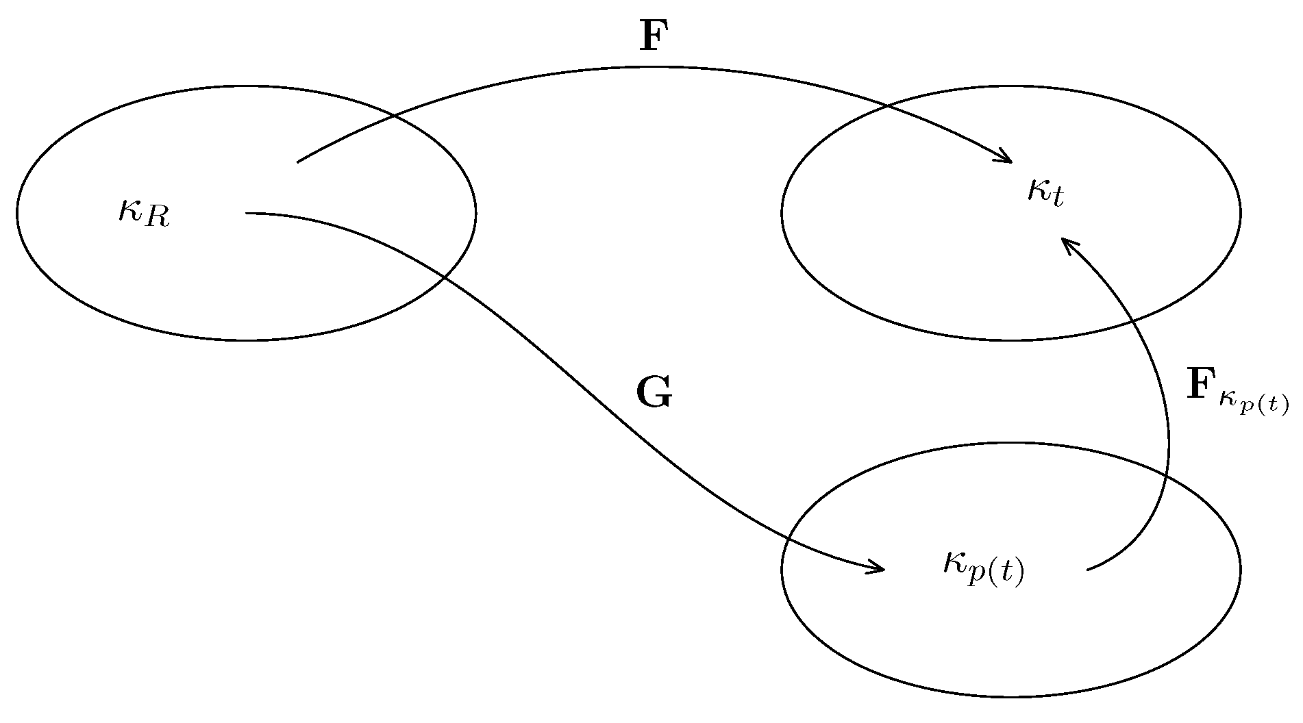
In this section, we consider a setting described by three configurations: reference, current and a natural one (see Figure 4). We first recall the derivation developed in [6,9,27] and then provide its extension. Throughout the rest of this paper, we suppose that
det F = 1 and div v = tr D = 0 ,
but F κ p ( t ) and G do not fulfill det F κ p ( t ) = 1 = det .
We assume that (compare with (36))
ψ = ψ ˜ ( ρ ) + G 2 ρ tr B κ p ( t ) 3 ln det B κ p ( t ) .
Inserting (50) into (21c), using also (14) and (43), we obtain
ξ = T δ G ( B κ p ( t ) ) δ · D δ + G ( κ p ( t ) I ) · D κ p ( t ) = : ξ 1 + ξ 2 .
This identity is the starting point for developing a plethora of models of the Maxwell type or the Oldroyd-B type. We say that the model is of Maxwell type if
T δ G ( B κ p ( t ) ) δ = 0 T = ϕ I + G B κ p ( t ) with ϕ : = m G tr B κ p ( t ) 3
and is of Oldroyd-B type if
T δ G ( B κ p ( t ) ) δ = 2 μ D δ T = ϕ I + 2 μ D + G B κ p ( t ) with ϕ : = m G tr B κ p ( t ) 3 .
One could decompose the dissipative term G ( κ p ( t ) I ) · D κ p ( t ) into the product of deviatoric parts and the product of traces (which would distinguish the dissipative contributions due to volume changing processes from the isochoric processes). The reason that we do not do so here is threefold. First, getting into these details would tend to hinder the clarity of the central ideas of the development. Second, it is unnecessary for the development of the rate-type models that are carried out in this work. Finally, the interested reader can find the consequences of splitting the dissipation in such a manner in [27] where it has been carried out systematically within the context of general compressible bodies.
In [9], Rajagopal and Srinivasa treat the case tr D κ p ( t ) = 0 (which is relaxed here and consequently (51) differs from the equation for ξ obtained in [9]), considering two types of dissipation connected with ξ 2 . First, the choice
G ( C κ p ( t ) I ) = 2 μ 1 D κ p ( t )
leads to
ξ 2 = 2 μ 1 | D κ p ( t ) | 2 .
Second, the choice
G ( κ p ( t ) I ) = 2 μ 1 D κ p ( t ) κ p ( t )
leads to
ξ 2 = 2 μ 1 D κ p ( t ) C κ p ( t ) · D κ p ( t ) = 2 μ 1 | D κ p ( t ) F κ p ( t ) | 2 .
The relation (54) and similarly the relation (56) are the identities that lead to rate-type equation for the stress as shown next.
Multiplying (56) from the left by F κ p ( t ) and from the right by F κ p ( t ) 1 , and recalling κ p ( t ) = F κ p ( t ) T F κ p ( t ) , we obtain
G ( B κ p ( t ) I ) = 2 μ 1 F κ p ( t ) D κ p ( t ) F κ p ( t ) T .
Using (14), we get
B κ p ( t ) + G μ 1 ( B κ p ( t ) I ) = 0 .
Recalling (52), (53) and setting : = G ( B κ p ( t ) I ) , we conclude that
T = p I + + 2 μ D with p = ϕ G , S + G μ 1 S = 2 G D μ 1 G S + S = 2 μ 1 D ,
where we have also used the fact that I = 2 D .
The model (60) with μ > 0 is the Oldroyd-B model [4], while (60) with μ = 0 is the Maxwell model.
On the other hand, multiplying (54) from the left by F κ p ( t ) and from the right by F κ p ( t ) T and using (14), we arrive at
B κ p ( t ) + G μ 1 ( B κ p ( t ) I ) B κ p ( t ) = 0 .
Setting again S : = G ( B κ p ( t ) I ) , we end up with
T = p I + + 2 μ D with p = ϕ G , S + G μ 1 S + 1 μ 1 S 2 = 2 G D μ 1 G S + S + 1 G S 2 = 2 μ 1 D ,
which is the fluid model due to Giesekus [30].
Both of the above models can be shown to be special cases of a more general model. In order to show this, we set (instead of (54) and (56))
G ( C κ p ( t ) I ) = 2 μ 1 D κ p ( t ) C κ p ( t ) λ , λ 0 .
This leads to
ξ 2 = 2 μ 1 D κ p ( t ) C κ p ( t ) λ · D κ p ( t ) = | D κ p ( t ) U κ p ( t ) λ | 2 ,
where U κ p ( t ) comes from the polar decomposition of F κ p ( t ) , i.e., F κ p ( t ) = R κ p ( t ) U κ p ( t ) .
Clearly, if λ = 0 , then we get the case leading to the Giesekus model, while, if λ = 1 , then we get the Maxwell/Oldroyd-B model depending on whether μ is zero/positive.
Now, multiplying (63) from the left by F κ p ( t ) and from the right by U κ p ( t ) 1 2 λ R κ p ( t ) T , we finally get
T = ϕ I + 2 μ D + G B κ p ( t ) , B κ p ( t ) + G μ 1 ( B κ p ( t ) I ) B κ p ( t ) 1 λ = 0 ,
which as discussed above generalizes the three-dimensional models developed by Maxwell, Oldroyd-B, Giesekus and includes them as special cases.
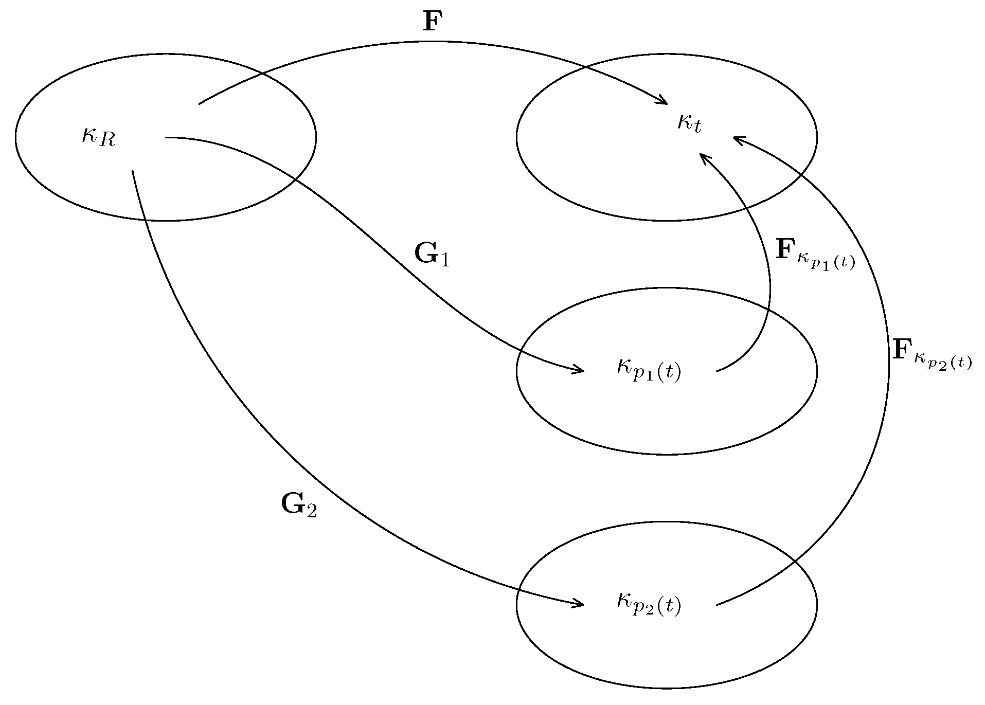
4. Burgers Model

Finally, we consider a setting wherein there are two evolving natural configurations associated with the body (see Figure 4 and kinematics summarized in (15)–(19)). Again, we assume that (49) holds and, motivated by the discussion in the preceding section, we assume that
ψ = ψ ˜ ( ρ ) + G 1 2 ρ tr B κ p 1 ( t ) 3 ln det B κ p 1 ( t ) + G 2 2 ρ tr B κ p 2 ( t ) 3 ln det B κ p 2 ( t ) .
Inserting (66) into (21c), using (18), (19) and (49), we obtain
ξ = T G 1 B κ p 1 ( t ) G 2 B κ p 2 ( t ) δ · D δ + G 1 ( C κ p 1 ( t ) I ) · D κ p 1 ( t ) + G 2 ( C κ p 2 ( t ) I ) · D κ p 2 ( t ) = : C ( D δ , D κ p 1 ( t ) , D κ p 2 ( t ) ) .
Next, as in Section 3, we postulate that
T G 1 B κ p 1 ( t ) G 2 B κ p 2 ( t ) δ = 2 μ D δ ,
G 1 ( C κ p 1 ( t ) I ) = 2 μ 1 D κ p 1 ( t ) C κ p 1 ( t ) λ 1 ,
G 2 ( C κ p 2 ( t ) I ) = 2 μ 2 D κ p 2 ( t ) C κ p 1 ( t ) λ 2 ,
which upon inserting these relations into (67), yields
ξ = 2 μ | D δ | 2 + 2 μ 1 D κ p 1 ( t ) C κ p 1 ( t ) λ 1 · D κ p 1 ( t ) + 2 μ 2 D κ p 2 ( t ) C κ p 2 ( t ) λ 2 · D κ p 2 ( t ) , μ , μ 1 , μ 2 > 0 , λ 1 , λ 2 0 .
Using the fact that C κ p i ( t ) = U κ p i ( t ) 2 , i = 1 , 2 , where U κ p i ( t ) is the right stretch tensor obtained from the polar decomposition of F κ p i ( t ) , i.e., F κ p i ( t ) = R κ p i ( t ) U κ p i ( t ) , we conclude from (49) and (71) that
ξ = 2 μ | D δ | 2 + 2 μ 1 | D κ p 1 ( t ) U κ p 1 ( t ) λ 1 | 2 + 2 μ 2 | D κ p 2 ( t ) U κ p 2 ( t ) λ 2 | 2 ;
thus, ξ 0 .
The constitutive equations for a class of Burgers models are obtained from (68)–(70) in the following way. We multiply (69) from the left by F κ p 1 ( t ) and from the right by U κ p 1 ( t ) 1 2 λ 1 R κ p 1 ( t ) T and we also multiply (70) from the left by F κ p 2 ( t ) and from the right by U κ p 2 ( t ) 1 2 λ 2 R κ p 2 ( t ) T . Referring to (18), we observe that Equations (68)–(70) lead to
T = ϕ I + 2 μ D + G 1 B κ p 1 ( t ) + G 2 B κ p 2 ( t ) with ϕ = m G 1 tr B κ p 1 ( t ) 3 G 2 tr B κ p 2 ( t ) 3 ,
B κ p 1 ( t ) + G 1 μ 1 ( B κ p 1 ( t ) 2 λ 1 B κ p 1 ( t ) 1 λ 1 ) = 0 ,
B κ p 2 ( t ) + G 2 μ 2 ( B κ p 2 ( t ) 2 λ 2 B κ p 2 ( t ) 1 λ 2 ) = 0 .
By choosing λ 1 = λ 2 = 1 , one gets
T = ϕ I + 2 μ D + G 1 B κ p 1 ( t ) + G 2 B κ p 2 ( t ) ,
B κ p 1 ( t ) + G 1 μ 1 ( B κ p 1 ( t ) I ) = 0 ,
B κ p 2 ( t ) + G 2 μ 2 ( B κ p 2 ( t ) I ) = 0 .
Next, following [6], we show that the model (74) is equivalent to the Burgers model (2). Indeed, first, we define S 1 : = G 1 ( B κ p 1 ( t ) I ) and S 2 : = G 2 ( B κ p 2 ( t ) I ) and S : = S 1 + S 2 . Using (74b) and (74c), we have
S = S 1 + S 2 = G 1 μ 1 S 1 G 2 μ 2 S 2 + 2 ( G 1 + G 2 ) D .
Applying the upper convected Oldroyd derivative to (75) and using (74b) and (74c) again, we obtain
S = G 1 μ 1 S 1 G 2 μ 2 S 2 + 2 ( G 1 + G 2 ) D = G 1 2 μ 1 2 S 1 + G 2 2 μ 2 2 S 2 2 G 1 2 μ 1 + G 2 2 μ 2 D + 2 ( G 1 + G 2 ) D .
Multiplying the Equation (75) by ( G 1 / μ 1 + G 2 / μ 2 ) , and adding the result to (76), we obtain
T = p I + 2 μ D + S with p = ϕ G 1 G 2 ,
S + G 1 μ 1 + G 2 μ 2 S + G 1 G 2 μ 1 μ 2 S = 2 G 1 G 2 1 μ 1 + 1 μ 2 D + 2 ( G 1 + G 2 ) D ,
which coincides with (2).
It is also worth mentioning how the Equation (73) looks for λ 1 = λ 2 = 0 :
T = ϕ I + 2 μ D + G 1 B κ p 1 ( t ) + G 2 B κ p 2 ( t ) ,
B κ p 1 ( t ) + G 1 μ 1 ( B κ p 1 ( t ) 2 B κ p 1 ( t ) ) = 0 ,
B κ p 2 ( t ) + G 2 μ 2 ( B κ p 2 ( t ) 2 B κ p 2 ( t ) ) = 0 .
When λ 1 = 1 and λ 2 = 0 , we obtain a model where one response corresponds to the Giesekus model and the other to the Maxwell model (note that the natural configurations are interchangable):
T = ϕ I + 2 μ D + G 1 B κ p 1 ( t ) + G 2 B κ p 2 ( t ) ,
B κ p 1 ( t ) + G 1 μ 1 ( B κ p 1 ( t ) 2 B κ p 1 ( t ) ) = 0 ,
B κ p 2 ( t ) + G 2 μ 2 ( B κ p 2 ( t ) I ) = 0 .
Finally, we show that the Equations (68)–(70), which represent the initial forms for the final structure of constitutive equations, can be obtained using the knowledge of how the material dissipates the energy and referring to the assumption that the material response is such that it maximizes the rate of entropy production.
Following the methodology outlined in Section 2.2, we first specify how the material dissipates the energy. Referring to (71), we set ξ ^ C κ p 1 ( t ) , C κ p 2 ( t ) ( D δ , D κ p 1 ( t ) , D κ p 2 ( t ) ) to be the function appearing on right-hand side of (71). Note that ξ ^ C κ p 1 ( t ) , C κ p 2 ( t ) ( D δ , D κ p 1 ( t ) , D κ p 2 ( t ) ) is in virtue of (72) non-negative, and is quadratic in D δ , D κ p 1 ( t ) , D κ p 2 ( t ) , and includes C κ p 1 ( t ) and C κ p 2 ( t ) as parameters. In the rest of this section, we simplify the notation by omitting the subscripts, i.e.,
ξ ^ ( D δ , D κ p 1 ( t ) , D κ p 2 ( t ) ) = ξ ^ C κ p 1 ( t ) , C κ p 2 ( t ) ( D δ , D κ p 1 ( t ) , D κ p 2 ( t ) ) .
In accordance with the scheme described in Section 2.2, we determine the constitutive equation by the maximization ξ ^ ( D δ , D κ p 1 ( t ) , D κ p 2 ( t ) ) over the set of D δ , D κ p 1 ( t ) , D κ p 2 ( t ) fulfilling
ξ ^ C κ p 1 ( t ) , C κ p 2 ( t ) ( D δ , D κ p 1 ( t ) , D κ p 2 ( t ) ) = C ( D δ , D κ p 1 ( t ) , D κ p 2 ( t ) ) ,
where C ( D δ , D κ p 1 ( t ) , D κ p 2 ( t ) ) is given in (67). This constrained maximization is performed by employing the Lagrange multiplier method. We set
L ( D δ , D κ p 1 ( t ) , D κ p 2 ( t ) ) = ξ ^ ( D δ , D κ p 1 ( t ) , D κ p 2 ( t ) ) + ξ ^ ( D δ , D κ p 1 ( t ) , D κ p 2 ( t ) ) C ( D δ , D κ p 1 ( t ) , D κ p 2 ( t ) ) ,
where is the Lagrange multiplier corresponding to the constraint (81). The necessary conditions for the extrema are
L D δ = 0 , L D κ p 1 ( t ) = 0 , L D κ p 2 ( t ) = 0 ,
which results in
1 + 4 μ D δ = T δ G 1 ( B κ p 1 ( t ) ) δ G 2 ( B κ p 2 ( t ) ) δ ,
1 + 2 μ 1 ( D κ p 1 ( t ) C κ p 1 ( t ) λ 1 + C κ p 1 ( t ) λ 1 D κ p 1 ( t ) ) = G 1 ( I κ p 1 ( t ) I ) ,
1 + 2 μ 2 ( D κ p 2 ( t ) C κ p 2 ( t ) λ 2 + C κ p 2 ( t ) λ 2 D κ p 2 ( t ) ) = G 2 ( C κ p 2 ( t ) I ) .
Upon taking the scalar product of (84a) with D δ and (84a) with D κ p 1 ( t ) and (84c) with D κ p 2 ( t ) and adding these results together, we obtain
1 + = ( T G 1 B κ p 1 ( t ) d G 2 B κ p 2 ( t ) d ) δ · D δ + i = 1 2 G i ( κ p i ( t ) I ) · D κ p i ( t ) 4 μ | D | 2 + 4 μ 1 D κ p 1 ( t ) C κ p 1 ( t ) λ 1 · D κ p 1 ( t ) + 4 μ 2 D κ p 2 ( t ) C κ p 2 ( t ) λ 2 · D κ p 2 ( t ) = ξ ^ 2 ξ ^ = 1 2 .
Then, it follows from (84a) (compare with (68)) that
T = m I + T δ = m I + 2 μ D δ + G 1 ( B κ p 1 ( t ) ) δ + G 2 ( B κ p 2 ( t ) ) δ .
Now, similar to the arguments advanced in [9], we show that C κ p i ( t ) λ i and D κ p i ( t ) commute. Let C κ p i ( t ) have an eigenvector e corresponding to an eigenvalue ϕ . Then, C κ p i ( t ) λ i has the same eigenvector e corresponding to the eigenvalue ϕ λ i . After substituting for , we apply both sides of 84b on e and obtain
μ i ( ϕ λ i I + C κ p i ( t ) λ i ) D κ p i ( t ) e = G i ( ϕ 1 ) e , i = 1 , 2 .
Since C κ p i ( t ) is positive definite, ϕ is positive and ϕ λ i I + κ p i ( t ) λ i is invertible with the same eigenvector e . Thus,
D κ p i ( t ) e = ϕ ˜ e ,
which means that e is also an eigenvector of D κ p i ( t ) . Thus, the tensors C κ p i ( t ) λ i and D κ p i ( t ) commute and we obtain relations given in (69) and (70), which we wished to show.

5. Conclusions

The models developed by Maxwell, Oldroyd and Burgers to describe the viscoelastic response of fluids are comprised of elastic and viscous responses. Recently, Rajagopal and Srinivasa [9] developed a thermodynamic framework wherein they assumed two scalar functions, the stored energy and the rate of entropy production, and assuming further that the rate of entropy production has to be maximized as the body undergoes deformation, they developed nonlinear models for viscoelastic fluids that are generalizations of the models due to Maxwell, Oldroyd and Burgers. When attention is restricted to incompressible viscoelastic fluids, the models developed by Rajagopal and Srinivasa [9], when the elastic response was linearized, in the sense that the displacement gradients are small so that the square of the norm of the displacement gradients can be ignored in comparison to the norm of the displacement gradient, leads exactly to the models developed by Maxwell, Oldroyd and Burgers. This might suggest that the models due to Maxwell, Oldroyd and Burgers allow only small elastic responses. In this paper, we show that this is not the case, provided we allow both the elastic and viscous responses to be non-isochoric while the combined response meets the condition of isochoricity. Such an assumption implies that an instantaneous elastic isochoric response as well as an instantaneous viscous response are not possible as we assume that the elastic response as well as the viscous response are not isochoric to begin with. The notion that a process can be instantaneous is an oxymoron as the word process implies something that takes time (the Oxford English Dictionary [31] defines process as “to go on” implying clearly something that takes time). Thus, one cannot expect any process to be instantaneous; however, we resort to the use of such processes in view of certain mathematical considerations (e.g., within the context of linear theories, this allows us to study the response to Heaviside functions using Laplace transforms). In this paper, we have shown that, in all other processes, the assumptions that are used lead to the models developed by Maxwell, Oldroyd and Burgers without having to resort to any approximation of the elastic response, that is, they are exactly the models developed by Maxwell, Oldroyd and Burgers.
We also introduced new generalizations (one-parameter families) of models of the Maxwell, Oldroyd and Burgers type that are compatible with the second law of thermodynamics.

Author Contributions

All three of the authors were equally involved in the formulation of the problem. The calculations were carried out by J.M. and K.T. The discussion of the results and the presentation of the material were carried out by all three of the authors.

Funding

J.M. and K.T. thank the Czech Science Foundation for the support through the project 18-12719S. K.T. has been supported by Charles University Research program No. UNCE/SCI/023.

Acknowledgments

J.M. and K.T. acknowledge the membership to the Nečas Center for Mathematical Modeling (NCMM). K.R.R. thanks the Office of Naval Research for its support.

Conflicts of Interest

The authors declare no conflict of interest.

References

  1. Narayan, S.P.A.; Krishnan, J.M.; Deshpande, A.P.; Rajagopal, K.R. Nonlinear viscoelastic response of asphalt binders: An experimental study of the relaxation of torque and normal force in torsion. Mech. Res. Commun. 2012, 43, 66–74. [Google Scholar] [CrossRef]
  2. Sharif-Kashani, P.; Hubschman, J.-P.; Sassoon, D.; Kavehpour, H.P. Rheology of the vitreous gel: Effects of macromolecule organization on the viscoelastic properties. J. Biomech. 2011, 44, 419–423. [Google Scholar] [CrossRef] [PubMed]
  3. Maxwell, J.C. On the dynamical theory of gases. Philos. Trans. R. Soc. 1867, 157, 49–88. [Google Scholar] [CrossRef]
  4. Oldroyd, J.G. On the formulation of rheological equations of state. Proc. R. Soc. Lond. Ser. A 1950, 200, 523–541. [Google Scholar] [CrossRef]
  5. Monismith, C.L.; Secor, K.E. Viscoelastic behavior of asphalt concrete pavements. In Proceedings of the International Conference on the Structural Design of Asphalt Pavements, Ann Arbor, MI, USA, 20–24 August 1962; Univ of California: Berkeley, CA, USA, 1962. [Google Scholar]
  6. Málek, J.; Rajagopal, K.R.; Tůma, K. A thermodynamically compatible model for describing the response of asphalt binders. Int. J. Pavement Eng. 2015, 16, 297–314. [Google Scholar] [CrossRef]
  7. Burgers, J.M. Mechanical considerations—Model systems—Phenomenological theories of relaxation and viscosity. In First Report on Viscosity and Plasticity; Nordemann Publishing: New York, NY, USA, 1939; Chapter 1; pp. 5–67. [Google Scholar]
  8. Rajagopal, K.R. Remarks on the notion of “pressure”. Int. J. Nonlinear Mech. 2015, 71, 165–172. [Google Scholar] [CrossRef]
  9. Rajagopal, K.R.; Srinivasa, A.R. A thermodynamic frame work for rate type fluid models. J. Non-Newton. Fluid Mech. 2000, 88, 207–227. [Google Scholar] [CrossRef]
  10. Rajagopal, K.R.; Srinivasa, A.R. On thermomechanical restrictions of continua. Proc. R. Soc. Lond. Ser. A Math. Phys. Eng. Sci. 2004, 460, 631–651. [Google Scholar] [CrossRef]
  11. Krishnan, J.M.; Rajagopal, K.R. Review of the uses and modeling of bitumen from ancient to modern times. Appl. Mech. Rev. 2003, 56, 149–214. [Google Scholar] [CrossRef]
  12. Krishnan, J.M.; Rajagopal, K.R. Triaxial testing and stress relaxation of asphalt concrete. Mech. Mater. 2004, 36, 849–864. [Google Scholar] [CrossRef]
  13. Karra, S.; Rajagopal, K.R. Development of three dimensional constitutive theories based on lower dimensional experimental data. Appl. Math. 2009, 54, 147–176. [Google Scholar] [CrossRef] [Green Version]
  14. Málek, J.; Rajagopal, K.R.; Tůma, K. A thermodynamically compatible model for describing the response of asphalt binders: Solutions of problems. Int. J. Pavement Eng. 2016, 17, 550–564. [Google Scholar] [CrossRef]
  15. Málek, J.; Rajagopal, K.R.; Tůma, K. On a variant of the Maxwell and Oldroyd-B models within the context of a thermodynamic basis. Int. J. Nonlinear Mech. 2015, 76, 42–47. [Google Scholar] [CrossRef]
  16. Málek, J.; Rajagopal, K.R. Mathematical issues concerning the Navier–Stokes equations and some of its generalizations. In Handbook of Differential Equations: Evolutionary Equations, vol. II; Elsevier/North-Holland: Amsterdam, The Netherlands, 2005; pp. 371–459. [Google Scholar]
  17. Málek, J.; Rajagopal, K.R. On the modeling of inhomogeneous incompressible fluid-like bodies. Mech. Mater. 2006, 38, 233–242. [Google Scholar] [CrossRef]
  18. Hron, J.; Miloš, V.; Průša, V.; Souček, O.; Tůma, K. On thermodynamics of incompressible viscoelastic rate type fluids with temperature dependent material coefficients. Int. J. Nonlinear Mech. 2017, 95, 193–208. [Google Scholar] [CrossRef] [Green Version]
  19. Bulíček, M.; Málek, J.; Průša, V. Thermodynamics and stability of non-equilibrium steady states in open systems. arXiv, 2017; arXiv:1709.05968. [Google Scholar]
  20. Dostalík, M.; Průša, V.; Tůma, K. Finite amplitude stability of internal steady flows of Giesekus viscoelastic rate-type fluid. arXiv, 2018; submitted. [Google Scholar]
  21. Feireisl, E.; Jin, B.J.; Novotný, A. Relative entropies, suitable weak solutions, and weak-strong uniqueness for the compressible Navier–Stokes system. J. Math. Fluid Mech. 2012, 14, 717–730. [Google Scholar] [CrossRef]
  22. Feireisl, E.; Novotný, A.; Sun, Y. A regularity criterion for the weak solutions to the Navier-Stokes-Fourier system. Arch. Ration. Mech. Anal. 2014, 212, 219–239. [Google Scholar] [CrossRef]
  23. Průša, V.; Rajagopal, K.R. Jump conditions in stress relaxation and creep experiments of Burgers type fluids: A study in the application of Colombeau algebra of generalized functions. Z. Angew. Math. Phys. 2011, 62, 707–740. [Google Scholar] [CrossRef]
  24. Hron, J.; Rajagopal, K.R.; Tůma, K. Flow of a Burgers fluid due to time varying loads on deforming boundaries. J. Non-Newton. Fluid Mech. 2014, 210, 66–77. [Google Scholar] [CrossRef]
  25. Tůma, K.; Stein, J.; Průša, V.; Friedmann, E. Motion of the vitreous humour in a deforming eye–fluid-structure interaction between a nonlinear elastic solid and a nonlinear viscoleastic fluid. Appl. Math. Comput. 2018, 335, 50–64. [Google Scholar] [CrossRef]
  26. Truesdell, C. A First Course in Rational Mechanics; Academic Press: Boston, MA, USA, 1991. [Google Scholar]
  27. Málek, J.; Průša, V. Derivation of Equations for Continuum Mechanics and Thermodynamics of Fluids. In Handbook of Mathematical Analysis in Mechanics of Viscous Fluids; Giga, Y., Novotny, A., Eds.; Springer: Cham, Switzerland, 2018. [Google Scholar]
  28. Bowen, R.M. Theory of Mixtures in Continuum Physics III; Eringen, A.C., Ed.; Academic Press: New York, NY, USA, 1976. [Google Scholar]
  29. Rajagopal, K.R.; Tao, L. Mechanics of Mixtures; World Scientific: River Edge, NJ, USA, 1995. [Google Scholar]
  30. Giesekus, H. A simple constitutive equation for polymer fluids based on the concept of deformation- dependent tensorial mobility. J. Non-Newton. Fluid Mech. 1982, 11, 69–109. [Google Scholar] [CrossRef]
  31. Oxford English Dictionary, 2nd ed.; prepared by Simpson, J.A., and Weiner, E.S.C.; Clarendon Press: Oxford, UK, 2000.
Figure 1. Lumped parameter system mechanical analog used by Burgers.
Fluids 03 00069 g001
Figure 2. (a) mechanical analog of a variant of the Burgers model; (b) mechanical analog of a variant of the Burgers model with an additional dashpot.
Fluids 03 00069 g002
Figure 3. Deformation gradient F maps an infinitesimal filament from the reference configuration κ R to the current configuration κ t .
Fluids 03 00069 g003
Figure 4. Using the natural configuration κ p ( t ) the deformation gradient F is split into instantaneous elastic response F κ p ( t ) and the response G associated with energy dissipation.
Fluids 03 00069 g004
Figure 5. Using two natural configurations, κ p 1 ( t ) and κ p 2 ( t ) , the total deformation F is split into purely elastic parts corresponding to the mappings F κ p 1 ( t ) , F κ p 2 ( t ) , and dissipative parts G 1 , G 2 .
Fluids 03 00069 g005

