Abstract
Roadside noise barrier helps to reduce downwind pollutant concentrations from vehicle emission. This positive characteristic of the construction feature can be explained by its interaction with flow distribution and species dispersion. In this paper, a three-dimensional numerical model has been developed to simulate highway pollutant dispersion—a realizable k-ε model was employed to model turbulent flow, and a non-reaction species dispersion model was applied to simulate species transport. First, numerical models were validated with experimental data, and good agreement was observed. Then, detailed simulations were conducted to study double barriers’ effects on highway pollutant dispersion under different settings: noise barriers with different heights, noise barriers with and without edge effects, and different atmospheric thermal boundary conditions. Results show that: (1) Noise barriers without edge effects cause bigger downwind velocity and turbulence intensity than noise barriers with edge effects. (2) At ground level, lower downwind pollutant concentration and higher pollutant concentration, near upwind barrier and between barriers, are observed for noise barriers without edge effect cases; higher on-road pollutant concentration can be seen near barrier side edges for cases with edge effect. (3) Downwind velocity and turbulence intensity increase as barrier height increases, which causes reduced downwind pollutant concentration. (4) With the same barrier height, under unstable atmospheric boundary condition, the lowest pollutant concentration can be found for both downwind and between barriers. Overall, these findings will provide valuable inputs to noise barrier design, so as to improve roadside neighborhood air quality.
1. Introduction
Vehicle exhaust contributes highly to air pollution, and causes the increase of fatal diseases, low birth rates, and other health problems. As a matter of fact, air pollution has been a consistent and vital issue around the world. China has been suffering from severe air pollution for the past decades, 70% of which is a result of motor vehicle emissions [1]. According to EPA, motor vehicles cause nearly 75% of carbon monoxide pollution in the United States [2]. Moreover, over 45 million people in the United States are estimated to live, work, or attend school within 90 m of roadways, where high concentrations of air pollution have been observed, due to motor vehicle emissions [3]. It is important to study highway contaminant dispersion to minimize the exposure to air pollution caused by vehicle emission.
Noise barriers were originally designed to reduce moving vehicles’ noise effects on roadside neighborhood. Studies have suggested that roadside barriers have positive effects on the reduction of downwind pollutant concentration [4,5,6,7,8,9,10,11,12,13,14]. The level of benefits can be influenced by many factors, such as roadway configuration, local meteorology, barrier height, or barrier edge design. Further detailed studies are necessary to understand the effects of determination factors. They will provide valuable inputs to noise barrier design, so as to improve roadside neighborhood air quality.
Related research has been conducted in different ways: wind tunnel experiments, field data collection, and numerical modeling. All of these have contributed to understanding relations between noise barriers and their influences on highway pollutant dispersion due to vehicle emissions.
A frequently referred to wind tunnel experiment was done by Heist et al. in 2009 [4]. It focused on the analysis of roadway elevation or depression effects, combined with different barrier heights. It emphasized the importance of considering roadway configuration to study near-road air quality. It demonstrated the concept of combining virtual origin shift and entrainment velocity function into dispersion modeling equation, for a better representation of different roadway configurations.
Field study is another popular approach to study roadside contaminant dispersion. It gives us accurate, realistic real-time data for further modeling and analysis. In 2009, Baldauf et al. studied the effects of noise barrier design on downwind contaminant concentration by analyzing collected data. They also gave an insight into the relation between roadside designs with contaminant plume rise, based on Heist wind tunnel data [5]. Similar results were suggested by Ning et al. in 2010 [6]. A downwind contaminant peak concentration was found at about 1.9–2.2 times the peak concentration at clearing site (no noise barrier case). Another field study done by Hagler, in 2012, studied the barrier effect under various wind conditions [7]. In 2009, Finn et al. conducted a study on noise barrier effect under various atmospheric stability conditions by a tracer experiment [8]. A field study was also conducted by Baldauf et al. in 2015. They analyzed the influence of noise barriers on both on-road and downwind pollutant concentrations near a highway [9].
Numerical simulation is cost-efficient compared with field study and wind tunnel experiments. Many researchers have conducted modeling and simulation of noise barrier effects on air pollution. In 2011, Hagler et al. [10] studied barrier height and wind direction effects on near-road air quality. In 2014, Schulte et al. evaluated the ability of two numerical models, and studied barrier height effects under different thermal stabilities [11]. Most recently, Lee et al. studied the combination of noise barrier and roadside vegetation effects on air pollution dispersion under various wind conditions, based on a field study in 2017 [12]. In 2018, Amini et al. studied effects of different roadway configurations on near-road contaminant dispersion [13]. Generally, a noise barrier will carry the same length as the length of a roadway. However, if a barrier length is shorter than the roadway length, edge effects will be introduced. Barriers’ vertical side edges can induce turbulence flow, that affects the downwind flow field. Noise barrier edge effects were first mentioned in 2013 by Steffen et al. [14]. The sensitivity study of wind direction and wind speed on pollutant transport was performed. They found that edge effect might cause secondary recirculation. It concluded that the edge effect gets stronger with higher wind speed. However, there were no further detailed analyses of results on noise barrier edge effects on pollutant dispersion, and no further studies about thermal effects either.
The purpose of this study is to analyze barriers’ vertical side edges and atmospheric boundary layer effects on wind flow field and pollutant dispersion near roadside. Simulation results will provide valuable input to roadside barrier design, and improve the roadside air quality.
2. Materials and Methods
This section describes theories and numerical models used in this study. Commercial software ANSYS/FLUENT 18.0 has been used in the simulation. Reynolds-averaged Navier–Stokes (RANS) equation is widely used to compute turbulence flow motion. It decomposes Navier–Stokes equations by separating one flow variable into the combination of a time-averaged mean component and a fluctuating component. This computational method is applied in this study due to its feasibility to simulate steady state turbulence flow and incompressible ideal gas transportation, and its efficiency, leading to manageable computational efforts. It gives a RANS equation as below:
where t is time, and are time-averaged mean velocity, is the Reynolds stress (i = 1, 2, 3, streamwise x, spanwise y, vertical z directions).
Realizable k-ε model is used for turbulent flow characteristics prediction due to its efficiency in iteration.
The governing equation for turbulence kinetic energy (TKE), k, is given as
The governing equation for turbulence dissipation rate (TDR), ε, is given as
where
is generated turbulence kinetic energy by mean velocity gradients; is generated turbulence kinetic energy by buoyancy; is the fluctuating component for considering incompressible flow contribution to dissipation rate; and are turbulent Prantl numbers; and are source terms [15].
Power law was used to generate inlet wind velocity profile.
Inlet power law wind profile, under neutral condition, was the same as the one used by Steffens [14]. Velocity was validated as u = 7.44 m/s (z = 3 m), u = 10.75 m/s (z = 30 m); .
In this study, the inlet flow properties for large Atmospheric Boundary Layer (ABL) domain fully developed flow are based on methods introduced in Pieterse, 2013 [16]. It assumes the flow over surface layer of a homogeneous flat terrain. Basic flow properties are based on Monin–Obukhov similarity theory, which describes dimensionless mean flow and mean temperature in the surface layer under non-neutral condition, as a function of the dimensionless height parameter , where L is defined as Monin–Obukhov length with the following form:
K is the von Karman constant, set to be 0.41 in this study; is friction velocity; is the scaling temperature which discretizes neutral, stable, and unstable atmosphere stability conditions.
Inlet temperature profile is given as [17]:
where is given by
Carbon dioxide () is the representative gasoline passenger car and diesel truck emission gas, defined as a contaminant source in this paper. The emission mass flow rate in both was approximately 0.006 kg/s, calculated by using the average emission data from the United States Environmental Protection Agency (US EPA) 2017 Carbon Dioxide Emissions and Fuel Economy Trends Report [18]. The average emission is 0.0002 kg/m (352 g/mi). Vehicle highway speed was estimated to be 30 m/s (65 mph).
A numerical equation for non-reaction species dispersion is given as
Yi is the local mass fraction of the species. Ri is the net rate of production of species i by chemical reaction, which equals to 0 in this study. Si is the rate of production from sources. This equation follows the similar continuity equation format as Eulerian dispersion model, with specified contaminants in molar concentration mol/m3 instead of mass fraction [19].
In this study, the computational domain has a dimension of L = 500 m, W = 180 m, and H = 100 m, as shown in Figure 1. Barrier has a 0.3 m width (W1) with various heights (1, 2, 3, and 4 m). Roadway was modeled as a 0.2 m-wide line source, as shown in Figure 1. The emission source was modeled as a line source of 0.1 m width. For non-edge effect geometry, barrier length extends through the entire domain (. For edge effect case, barriers have a length of 50 m, smaller than domain (. The detailed barrier geometry with edges is shown in Figure 1c.
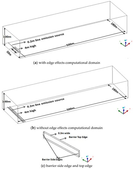
Figure 1.
Computational domain for noise barriers (a) with edge effects, (b) without edge effects, and (c) close view of the noise barrier.
Boundary conditions used in neutral condition simulations are listed in Table 1. Domain inlet is set to be velocity inlet with numerical wind profile derived from user defined function (UDF). Outlet is set to be outflow condition. Side walls are set to be symmetry conditions. Domain top is set to be non-shear slip wall without considering shear stress. Barriers and bottom are all set to be non-slip wall with proper roughness constants and roughness heights.

Table 1.
Boundary conditions for neutral condition.
3. Results
3.1. Model Validation
Computational domain for wind profile validation is shown in Figure 2, same as the one used by Steffens et al. [14]. Results were compared with Steffens’ and Near Road Tracer Study (NRTS08) experimental data and simulation results by using RANS turbulence model. A comparison of velocity profiles at 24 m downwind is shown in Figure 3. The velocity profile in this study has great similarity to the reference velocity profile. The line trend falls very close to the experimental data trend.
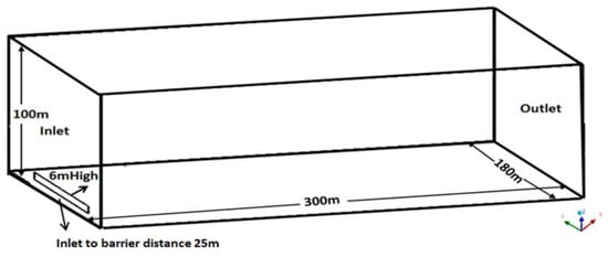
Figure 2.
Wind profile validation computational domain.
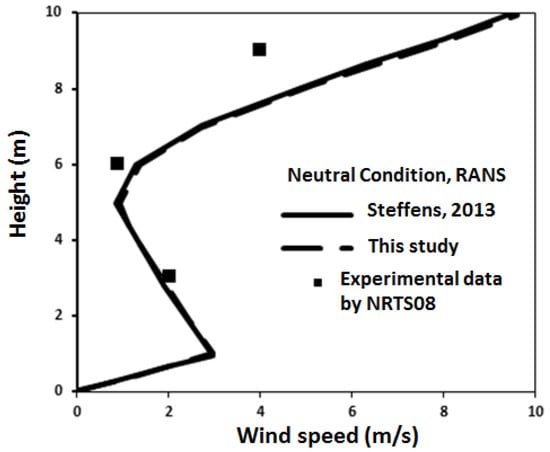
Figure 3.
Vertical velocity distribution comparison at 24 m downwind from inlet.
Atmosphere boundary layer has different thermal stabilities due to the change of air temperature deviations. The different thermal stabilities have impacts on pollutant dispersion due to buoyancy effects. Figure 4 shows comparisons of the inlet temperature vertical distributions against theoretical data and simulation results introduced in [16] by Pieterse et al.
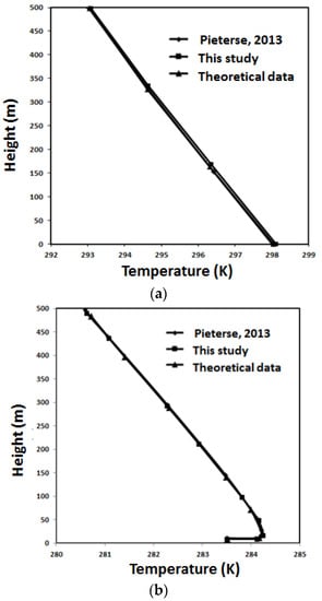
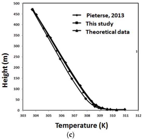
Figure 4.
Inlet temperature vertical distribution comparisons against theoretical profiles (a) neutral condition, (b) stable condition, and (c) unstable condition.
To validate the contamination dispersion model used in this study, simulation settings were taken, which are similar those in the wind tunnel experiment introduced by Heist, 2009 [4]. In this experiment, a multiple roadway configuration was used. It modeled a 6-lane highway system, with emission line source up along the lanes with SF6 gas. In a wind tunnel, it creates the wind profile based on collected field experiment data. Emission source has a mass flow rate of 0.01 kg/s. Inlet turbulent properties profiles are modified according to wind tunnel experiment input data. Figure 5 shows the comparison of the normalized concentration versus the change of the dimensionless downwind distance at ground level z = 1 m, where h represents the height of the noise barrier. Good agreement was observed with experimental data.
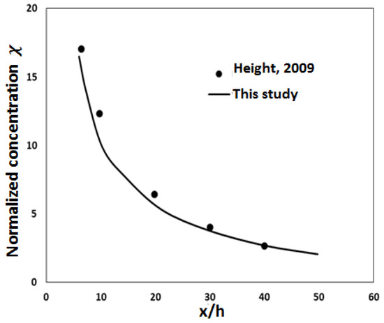
Figure 5.
Comparison of normalized concentration.
3.2. Numerical Analysis of Barrier Edge Effect under Neutral Condition
Flow Characteristics Comparison between Edge Effects and Non-Edge Effects
In this section, simulation results of flow characteristics, such as velocity, turbulence intensity, and turbulence kinetic energy (TKE), are compared for cases with and without barrier edge effects. Various barrier heights are adopted (1, 2, 3, and 4 m).
Figure 6 shows velocity streamline in the middle iso-surface (Y = 90 m). The plotted area has a 100 m horizontal span in X axis direction, and 10 m vertical height in Z axis direction.
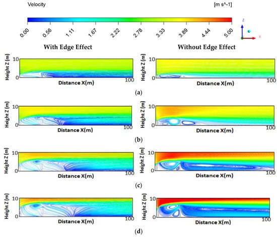
Figure 6.
Comparison of streamline in symmetry plane (Y = 90 m) for barrier geometry with and without edge effects at different barrier heights under neutral condition. The noise barrier height is (a) 1 m, (b) 2 m, (c) 3 m, and (d) 4 m.
As shown in Figure 6, flow starts to accelerate on the top of upwind barriers. A low speed zone is formed between barriers. Flow starts to decelerate as the wind passes the downwind barrier, and tends to recover further downwind. The maximum velocity increases as barrier height increases. The behavior of flow induces negative pressure zone between barriers and behind downwind barrier. A wake region is formed, which has a low speed, low pressure, and high turbulence level flow recirculation.
Due to the existence of flow recirculation, the flow field of non-edge effect barriers’ geometry has a vortex region, generated between barriers and behind the downwind barrier. In between barriers, multiple vortex regions are generated. A vortex near the bottom right corner of barriers grows as the barrier height increases. Similarly, a wake region of vortex is formed behind the downwind barrier. The size of the wake region grows as the barrier height increases. The center of the wake is shifted further away from the barrier, horizontally, as barrier height increases.
For edge effect cases, only one vortex region can be seen near the top of the downwind barrier. It can also be noticed that the size of the vortex increases as the barrier height increases. No complete vortex region can be found behind the downwind barrier. This is caused by the mixing flow induced by the side edges of the noise barriers. At the same barrier height, maximum velocity is smaller than that in the non-edge effect cases.
Figure 7 shows another group of streamline profiles for two barrier geometries. However, the plotted surface is 10 m offset from the middle plane in Y direction (Y = 80 m). A great similarity of velocity distribution can be seen for non-side edge effect cases. It shows that the velocity distribution is maintained the same in the lateral span of the entire computational domain (Y-direction) without considering barrier side edge effects. However, we can see different flow patterns for cases with side edge effects at plane Y = 80 m. A complete single vortex is formed between barriers. In the area behind the downwind barrier, a complete recirculation zone is also formed. Middle plane Y = 90 m is the symmetry plane of the computational domain and barrier geometry. Flow pattern within symmetry plane varies from flow pattern in non-symmetry plane for cases with side edge effects.
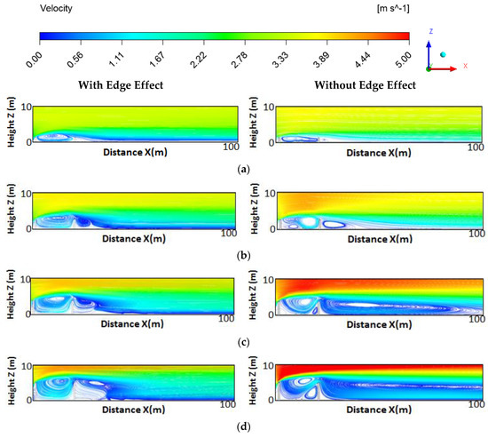
Figure 7.
Streamline at plane Y = 80 m (10 m offset from symmetry plane) for comparing effects of barrier geometry with and without side edges under neutral condition. The noise barrier height is (a) 1 m, (b) 2 m, (c) 3 m, and (d) 4 m.
Figure 8 and Figure 9 are contour plots of turbulence intensity. Turbulence intensity represents turbulence level. It is defined as the ratio of root-mean-square of the turbulent velocity fluctuations to Reynolds-averaged mean velocity. Figure 8 shows the contour of turbulence intensity in symmetry plane, for with and without side edge effect cases, while Figure 9 shows contour in plane Y = 80 m (10 m offset from the middle plane in Y direction). A similar turbulence intensity distribution can be found for cases without barriers in both planes. For barriers with side edges introduced, turbulence intensity distribution in the symmetry plane, shown in Figure 8, differs from that in the non-symmetry plane, shown in Figure 9. Higher turbulence intensity tends to appear in the symmetry plane for barriers with side edge effects. The maximum turbulence intensity tends to be located near the top of the downwind barrier for all conditions. Lower turbulence intensity can be found near the barrier bottom. Also, without barrier side edge effect cases have relatively smaller turbulence intensity at downwind ground level for all barrier heights. However, higher turbulence intensity between barriers can be seen for with side edge effect cases.
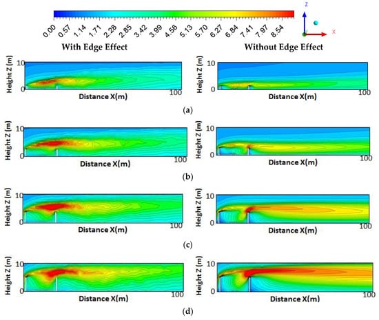
Figure 8.
Contour of turbulence intensity in symmetry plane (Y = 90) for comparing with and without side edges under neutral condition. The noise barrier height is (a) 1 m, (b) 2 m, (c) 3 m, and (d) 4 m.
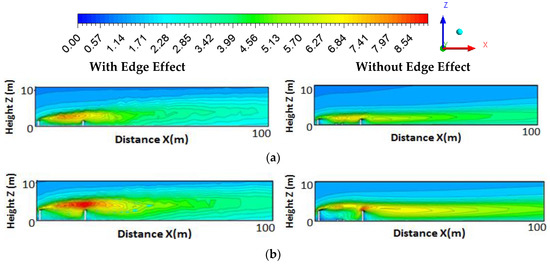
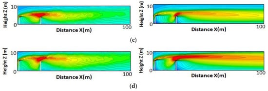
Figure 9.
Contour of turbulence intensity at plane Y = 80 for comparing with and without side edges under neutral condition. The noise barrier height is (a) 1 m, (b) 2 m, (c) 3 m, and (d) 4 m.
Figure 10 is a vertical profile of turbulence kinetic energy in the symmetry plane (Y = 90 m) at X = 100 m for with and without side edge effect cases. For both cases, peak turbulence kinetic energy value increases as barrier heights increase. However, for barriers with edge effects at the same height level, the turbulence kinetic energy is higher. The biggest difference happens with 1 m barrier height cases. Peak turbulence kinetic energies are listed in Table 2, for with and without barrier edge effect cases.
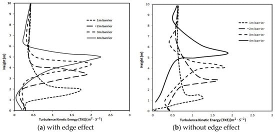
Figure 10.
Turbulence kinetic energy vertical profile in the symmetry plane.
Table 2.
Comparison of the peak turbulence kinetic energy (TKE) in the symmetry plane for with and without edge effect cases.
3.3. Pollutant Dispersion Characteristics under Neutral Condition
In the previous section, we discussed how flow characteristics are affected by the existence of barrier side edges in downwind region and between noise barriers. Compared with non-side edge effect barrier configuration, flow distribution along the Y direction has a different pattern, due to the existence of side edge-induced secondary turbulence. Turbulence intensity can be represented by the turbulence kinetic energy of the flow. Turbulence kinetic energy is a buoyancy-produced term that is directly determined by advections and dissipation rate. The concentration of a passive pollutant is determined by the horizontal advection, vertical advection, horizontal diffusion, vertical diffusion, and source or sink of pollutants [20]—pollutant dispersion is affected by flow field. In this section, we will discuss the effects of flow field and the barrier edge on pollutant dispersion.
Figure 11 shows the contour of pollutant dispersion in a symmetry plane (Y = 90 m). It can be seen that the noise barrier can reduce the pollutant concentration of the downwind region. A difference in downwind concentration can also be seen for with and without edge effect cases. Higher pollutant concentrations can be found in downwind locations for cases with side edge effect. In the area between barriers, side edge cases have lower pollutant concentrations than non-side edge cases. In Figure 8, higher turbulence intensity between barriers and lower turbulence intensity downwind can be found for side edge effect cases at the symmetry plane (Y = 90 m). Wind speed and turbulence intensity determine turbulent mixing and flow intensity. Those flow features will directly affect pollutant dispersion. Higher turbulence intensity and wind speed help pollutant dispersion faster.
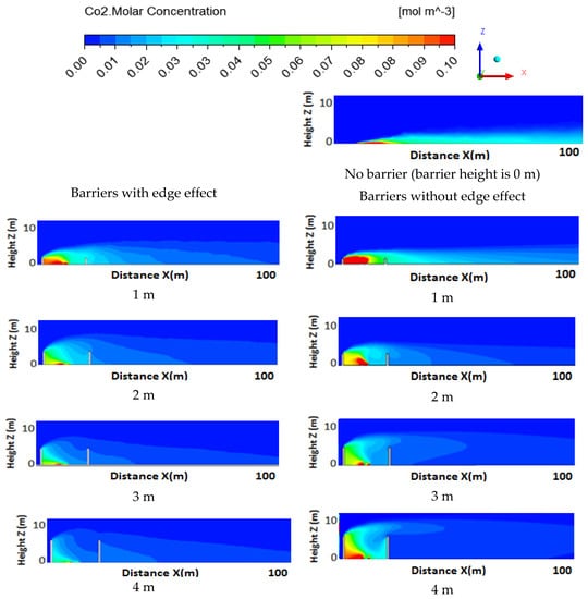
Figure 11.
concentration at different downwind distances within 10 m height.
Figure 12 gives a top view of concentration in the X–Y plane at ground level (Z = 1 m). It gives a clear view of concentration distribution for the on-road region between barriers and downwind behind barriers. High concentration zones can be seen between barriers, due to pollutant trapped by flow recirculation. For the 2, 3 and 4 m barriers with side edge effect cases, high concentrations in regions between barriers are separated into two zones, and the high concentration region between barriers for 1 m barrier height barely get separated. It can be seen that side edges do not show apparent effects on the 1 m barrier height case. Side edge impact increases as barrier height increases. Higher on-road concentration can be seen near barrier edges for with edge effect cases. This concentration distribution pattern follows the flow field distribution pattern between barriers, as discussed in the previous section. The highest concentration can be found at the vortex center.
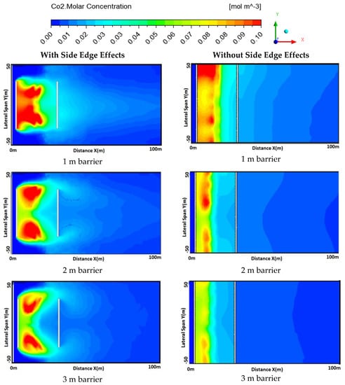
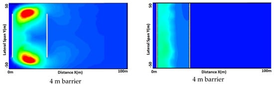
Figure 12.
concentration for with and without side edge effect cases in X–Y plane at ground level.
For non-side edge cases, it can be seen that a high concentration occurs near the upwind barrier at all heights, the highest pollutant concentration decreases as the barrier height increases, the high concentration region is not separated between barriers, and a relatively uniform concentration distribution can be seen between barriers and downwind.
Figure 13 depicts a concentration profile 10 m behind the downwind barrier for edge effect cases. Contaminant concentration decreases as the height of the noise barrier increases. Most profiles do not follow Gaussian shape distribution. However, with the 1 m barrier, the concentration near the barrier shows a shape similar to a Gaussian distribution. The concentration profile near the barrier is strongly affected by edge effects. Those effects increase as the height of the noise barriers increase.
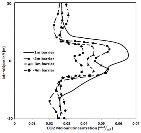
Figure 13.
concentration profile at downwind X = 10 m.
Further downwind at location X = 100 m, with a different barrier height, the concentration profiles are shown in Figure 14. For edge effect cases, all the concentration profiles at different barrier heights follow a similar shape as a Gaussian distribution. A peak concentration can be found for all barrier heights at the symmetry plane. The peak concentration value decreases as the barrier height increases. The 1 m barrier case has a maximum peak concentration of about 0.014 mol/m3, and the 4 m barrier case has a minimum peak concentration of about 0.009 mol/m3. Figure 14b shows concentration profiles with different barrier heights for without edge effect cases. An almost uniform distribution of concentration can be observed.
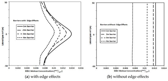
Figure 14.
concentration profile at downwind X = 100 m.
In order to further verify that the concentration distribution in the wake region for edge effect cases follows a Gaussian shape pattern, a self-similar concept was used for the concentration profile against normalized radial distance from the center of the wake (). The concept was adopted as described by Abkar et al. [21]. For the case where the downwind location x satisfies x/ > 4, the self-similar concentration profile is expected to collapse into a single Gaussian curve, except at the edge of the wake. X axis is , where is the entire barrier length ( = 50 m in this study) and is half of barrier length. Y axis is the normalized concentration ratio . Results show that, at different downwind locations for the same barrier height, concentration follows a single Gaussian shape distribution, as shown in Figure 15. This validated the self-similar Gaussian shape of concentration at certain downwind locations. It can be seen that, for different barrier heights, the Gaussian curve follows the same trend for the two downwind locations . H is the barrier heights 1, 2, and 3 m.
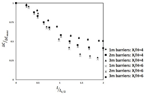
Figure 15.
Self-similar pollutant concentration profiles at different downwind locations at different barrier heights.
3.4. Barrier Edge Effect under Various Thermal Conditions
Figure 16 shows concentration contours at various barrier heights under different thermal stability conditions for with side edge effect cases.
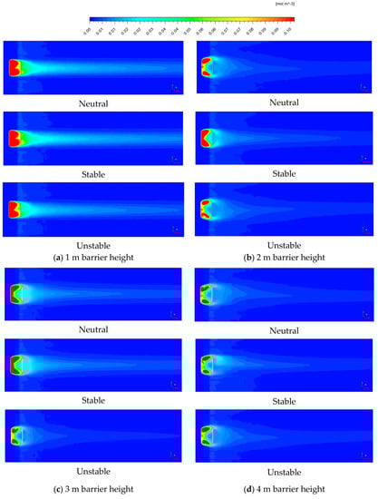
Figure 16.
Ground level (Z = 1 m) concentration for with edge effects under various thermal conditions for various noise barrier height.
Results show that the unstable condition has the lowest concentration at all barrier heights, while the stable condition has the highest concentration. The unstable condition has a stronger turbulence mixing effect on flow field. This leads to a faster flow velocity recovery on separated flow, which results in faster pollutant dispersion and lower pollutant concentrations.
4. Discussion
A 3-D numerical model was developed to simulate barrier side edge effects on pollutant dispersion. Simulations were conducted for flow and contaminant dispersion distribution, for on-road and downwind highway regions. The effects of various barrier heights, with and without barrier side edge effects and various atmospheric thermal boundary conditions, were analyzed.
Numerical models were first validated with experimental and theoretical data. Second, simulations were conducted, which focused on the neutral condition, to study how barrier side edges affect flow properties such as velocity, turbulence intensity, and turbulence intensity. Third, the effects on pollutant concentration distribution, from different atmospheric thermal conditions (neutral, stable, and unstable), were analyzed.
To consider the concentration distribution, simulation results for two regions were analyzed: on-road region (area between barriers) and downwind region (behind downwind barrier). For downwind region, higher velocity magnitude and turbulence intensity can be found for cases without side edge effect. This explains why less pollutant dispersion is observed at downwind region for without side edge cases. In the on-road region, at ground level, higher pollutant concentrations can be seen near barrier edges for with edge effect cases. With 1 m barrier, the side edge impact is not strong enough to separate flow between barriers. Overall, the ground level concentration decreases as barrier height increases, for both cases.
Considering the different thermal boundary effects, downwind wind velocity recovers fastest under unstable condition, compared with the neutral condition and stable condition. It was also found that unstable condition causes the lowest downwind concentration, and stable condition results in the highest downwind concentration with the same barrier height. Detailed simulation results will provide valuable inputs to determine noise barrier design and layout strategy, which can lead to reduced contaminant dispersion, pollutant concentration, and improvement of the air quality near highways.
Author Contributions
Conceptualization, X.W.; Simulation, L.G.; Writing-Original Draft Preparation, L.G.; Writing-Review & Editing, X.W.; Supervision, X.W.
Funding
This research received no external funding.
Conflicts of Interest
The authors declare no conflict of interest.
References
- Pressbooks. Available online: https://ohiostate.pressbooks.pub/sciencebites/chapter/causes-and-consequences-of-air-pollution-in-beijing-china/ (accessed on 1 May 2018).
- EPA. Available online: https://www.epa.gov/newsreleases/us-epa-partners-study-roadside-vegetation-and-air-quality-local-school (accessed on 1 May 2018).
- EPA. Available online: https://www.epa.gov/sites/production/files/2015-10/documents/ochp_2015_near_road_pollution_booklet_v16_508.pdf (accessed on 1 May 2018).
- Heist, D.K.; Perry, S.G.; Brixey, L.A. A wind tunnel study of roadway configurations on the dispersion of traffic-related pollution. Atmos. Environ. 2009, 43, 5101–5111. [Google Scholar] [CrossRef]
- Baldauf, R.; Thoma, E.; Khlystov, A.; Isakov, V.; Bowker, G.; Long, T.; Snow, R. Impacts of noise barriers on near-road air quality. Atmos. Environ. 2008, 42, 7502–7507. [Google Scholar] [CrossRef]
- Ning, Z.; Huddaa, N.; Dahera, N.; Kam, W.; Herner, J.; Kozawa, K.; Mara, S.; Sioutas, C. Impact of roadside noise barriers on particle size distributions and pollutants concentrations near freeways. Atmos. Environ. 2010, 44, 3118–3127. [Google Scholar] [CrossRef]
- Hagler, G.S.W.; Lin, M.Y.; Khlystov, A.; Baldauf, R.W.; Iskov, V.; Faircloth, J.; Jackson, L.E. Field investigation of roadside vegetative and structural barrier impact on near-road ultrafine particle concentrations under a variety of wind conditions. Sci. Total Environ. 2012, 419, 7–15. [Google Scholar] [CrossRef] [PubMed]
- Finn, D.; Clawson, K.L.; Roger, R.G.; Rich, J.D.; Eckman, R.M. Tracer studies to characterize the effects of roadside noise barriers on near-road pollutant dispersion under varying atmospheric stability conditions. Atmos. Environ. 2010, 44, 204–214. [Google Scholar] [CrossRef]
- RBaldauf, W.; Iskov, V.; Deshmarkh, P.; Venkatram, A.; Yang, B.; Zhang, K.M. Influence of solid noise barriers on near-road and on-road air quality. Atmos. Environ. 2016, 129, 265–276. [Google Scholar] [CrossRef]
- Hagler, G.S.W.; Tang, W.; Freeman, M.J.; Heist, D.K.; Perry, S.J.; Vette, A.F. Model evaluation of roadside barrier impact on near-road air pollution. Atmos. Environ. 2011, 45, 2522–2530. [Google Scholar] [CrossRef]
- Schulte, N.; Snyder, M.; Isacov, V.; Heist, D.; Venkatram, A. Effects of solid barriers on dispersion of roadway emissions. Atmos. Environ. 2014, 97, 286–295. [Google Scholar] [CrossRef]
- Lee, E.S.; Ranasinghe, D.R.; Ahangar, F.E.; Amini, S.; Mara, S.; Choi, W.; Paulson, S.; Zhu, Y. Field evaluation of vegetation and noise barriers for mitigation of near-freeway air pollution under variable wind conditions. Atmos. Environ. 2018, 175, 92–99. [Google Scholar] [CrossRef]
- Amini, S.; Ahangar, F.; Heist, D.; Perry, S.; Venkatram, A. Modeling Dispersion of Emissions from Depressed Roadways. Atmos. Environ. 2018, 186, 189–197. [Google Scholar] [CrossRef]
- Steffens, J.T.; Heist, D.K.; Perry, S.G.; Zhang, K.M. Modeling the effects of a solid barrier on pollutant dispersion under various atmospheric stability conditions. Atmos. Environ. 2013, 69, 76–85. [Google Scholar] [CrossRef]
- ANSYS. 14.1.1 Species Transport Equation. In ANSYS FLUENT 18.1 Theory Guide; ANSYS, Inc.: Canonsburg, PA, USA, 2017. [Google Scholar]
- Pieterse, J.E.; Harms, T.M. CFD investigation of atmospheric boundary layer under different thermal stabilities conditions. J. Wind Energy Ind. Aerodyn. 2013, 121, 82–97. [Google Scholar] [CrossRef]
- Alinot, C.; Masson, C. Aerodynamic Simulations of Wind Turbine Operating in Atmospheric Boundary layer with Various Thermal Stratifications. In Proceedings of the 2002 ASME Wind Energy Symposium, Reno, NV, USA, 14–17 January 2002. [Google Scholar]
- Executive Summary. Light-Duty Automotive Technology, Carbon Dioxide Emissions, and Fuel Economy Trends: 1975 Through 2017; EPA, EPA-420-S-18-001; EPA: Washington, DC, USA, January 2018. [Google Scholar]
- ANSYS. 17.5 Eulerian Model. In ANSYS FLUENT 18.1 Theory Guide; ANSYS, Inc.: Canonsburg, PA, USA, 2017. [Google Scholar]
- Hussian, M.; Lee, B.E. An Investigation of Wind Forces on Three-Dimensional Roughness Elements in a Simulated Atmospheric Boundary Layer Flow. Part II: Flow over Large Arrays of Identical Roughness Elements and the Effect of Frontal and Side Aspect Ratio Variants; University of Sheffield Department of Building Science Rep. BS-56; University of Sheffield: Sheffield, UK, 1980; 81p. [Google Scholar]
- Abkar, M.; Porte-Agel, F. Influence of Atmospheric Stability on Wind-Turbine Wakes: A Large-Eddy Simulation Study. AIP Phys. Fluids 2015, 27, 035104. [Google Scholar] [CrossRef]


© 2018 by the authors. Licensee MDPI, Basel, Switzerland. This article is an open access article distributed under the terms and conditions of the Creative Commons Attribution (CC BY) license (http://creativecommons.org/licenses/by/4.0/).