Theoretical Modeling, Design and Simulation of an Innovative Diverting Valve Based on Coanda Effect

Abstract

The present work is focused on the study of an innovative fluidic device. It consists of a two-ways diverter valve able to elaborate an inlet water flow and divert it through one of the two outlets without moving parts but as a result of a fluctuation of pressure induced by two actuation ports, or channels. Such apparatus is named Attachment Bi-Stable Diverter (ABD) and is able to work with the effect of the fluid adhesion to a convex wall adjacent to it, this phenomenon is known as Coanda Effect; it generates the force responsible for the fluid attachment and the consequent deviation. The main purpose of this work is to develop a knowhow for the design and development of such particular device. A mathematical model for the ABD has been developed and used to find the relationships between the geometrical parameters and the operative conditions. A configuration has been designed, simulated with a computational fluid dynamics approach. A prototype has been printed with and additive manufacturing printer and tested in laboratory to check the effective working point of the device.

1. Introduction

A “fluidic-device” is a particular apparatus able to take advantage of the interaction between fluid flows and nearby walls to produce a specific effect on the flow; this can be a deviation, or a turbulence/vorticity gain or an entrainment effect. The apparatus under study, said “fluidic-element”, works with a low amount of fluid flow at high speed and without moving parts, as clearly explained with many examples by Tesar [1]. It can elaborate on a relevant fluid flow power with low activation energy requirement. These devices are therefore reliable and can be very small, light and simple in their layout. For these reasons, such devices are very interesting for both the scientific and the industrial communities. Fluidic devices find applications in many industrial sectors, starting from the medical, through the hydraulics to the aerospace and propulsion technologies. This is because they can manage fluids in an innovative and less invasive way, compared to the traditional valves or actuators. The main shortcoming for its development consists in the presence of complex flow phenomena based on instable equilibrium that needs specific mathematical modeling and design knowledge.

The present work is based on a particular kind of fluidic element, called “Attachment Bi-stable Diverter”. Such device is part of a quite large class of fluidic elements that make use of the Coanda effect in order to manage a fluid flow direction change and to divert it from an inlet port to a desired outlet port. The input energy used by these devices is a perturbation of pressure that can break the equilibrium of the Coanda effect and drive the system to a new stable condition. This is the reason for the name “bi-stable”: the system can handle two different conditions of fluid flow stability depending on the outlet port activation. Henry Coanda was the first scientist to observe, study and identify the effect between the 1960s and the 1970s. This physical effect regards the interaction that takes place between a fluid jet and a nearby wall or two nearby fluid jets with different velocities. It allows the fluid flow to modify its direction before the interaction region, due to an equilibrium of only centrifugal force and pressure gradient acting on the jet. Thanks to the theoretical modeling both of the Coanda-effect and the off-set jets, a very reliable model of the fluidic device has been developed by the authors. It allows the prediction of the main operative parameters with good accuracy.

The theoretical study and mathematical modeling of the Coanda-driven fluidic elements is difficult and delicate because the complex fluid dynamics of the Coanda effect is exacerbated by the presence of turbulent effects due to the high Reynolds number. Many authors [2,3,4] demonstrated that a very tight relationship exists between the design criteria of a specific apparatus with its fluid dynamics. It is therefore difficult to develop a general design model, for the multiple variants of the geometric parameters that can have a strong influence on the device operation. On the simulation side, a difficult aspect is the proper setting of the computational fluid dynamics approach in order to accurately capture the flow mechanisms in the Coanda effect. Special attention is given not only to high quality mesh generation but also to the turbulent model selection (that cope with separated flows) has been devoted to the CFD model.

2. Study on the Attachment Bi-Stable Diverter (ABD)

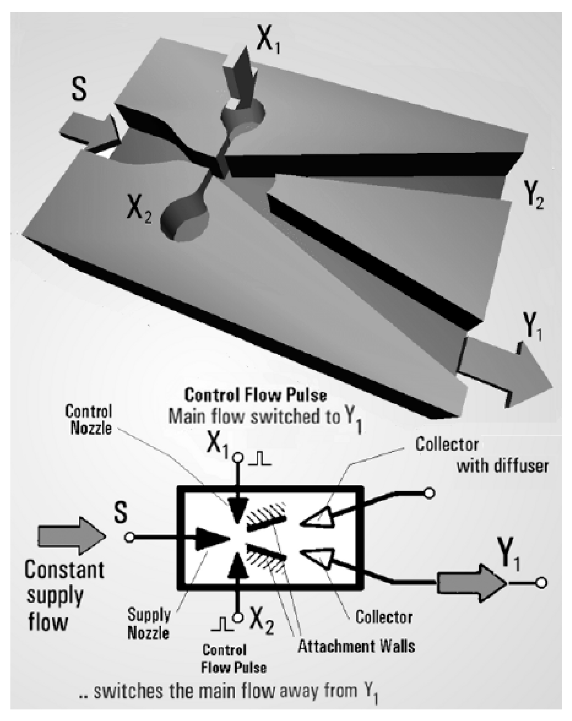
An ABD can be defined as a fluidic apparatus provided with one inlet port and two outlet ports for the main fluid; it has also two auxiliary ports, or actuation ports, for the command fluid. Such apparatus is able to divert the main stream from the inlet port to one selected outlet port by the fluid adhesion to the respective wall, as a result of the Coanda effect. Being this condition stable for both outlets this apparatus can also be defined as “bi-stable”. In fact, there are two symmetrical equilibrium conditions for the flow that can be broken by a perturbation induced through the auxiliary ports. The actuation induced by the auxiliary port drives the device into a transitional regime of flow called “switching-phase”. Once the switching phase begins, the flow detaches from a nearby wall and diverts its direction and it reattaches on the opposite nearby wall, symmetrical to the other one. In Figure 1, the geometrical configuration of the ABD is represented.

The inlet port of the main fluid is called S, then the two ports Xi are the auxiliary ports used to induce the perturbation in the main stream, while the ports Yi are the two outputs for the main flow. The ABD can be assimilated to a Y-conduit where the actuation ports are positioned at the cross of the channels, just before the convergent nozzle. 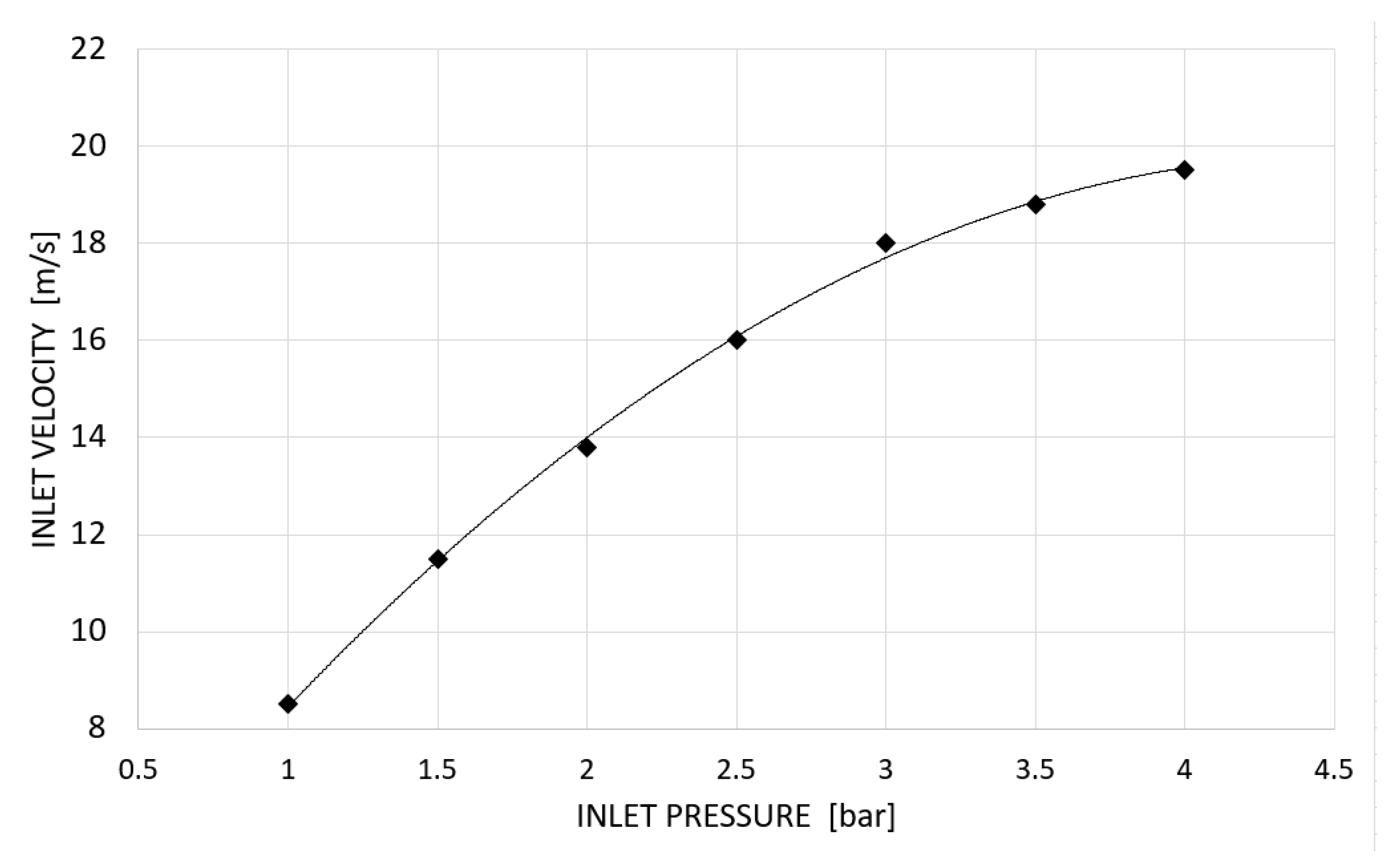The problem is modeled in 2D and the 3D duct of the fluidic apparatus is obtained by extrusion of the cross-sectional profile, as showed in Figure 1. Starting by defining the limits of the ABD operating region, an inlet relative pressure interval from 1 bar to 4 bar, and a volumetric flow target of 300 liters per hour have been fixed. The reference value of the area at the nozzle can be computed using the velocity:

$$U_{\max }= \sqrt{2\frac{\left(p_{\mathrm{in}}-p_{\mathrm{out}}\right)}{\rho }}$$

(1)

With the above data, a passage area of 4 mm² is obtained. The Reynolds number can be calculated in this section:

$$R{e}_h=\frac{U_{\max }\times h}{\nu }$$

(2)

were h is the height of the cross area at the nozzle, that has a square geometric profile h × h, and is equal to 2 mm. From Equation (2) a Reynolds number interval from 2 × ${10}^4$ to 6 × 10⁴, typical of a fully turbulent flow regime is considered.

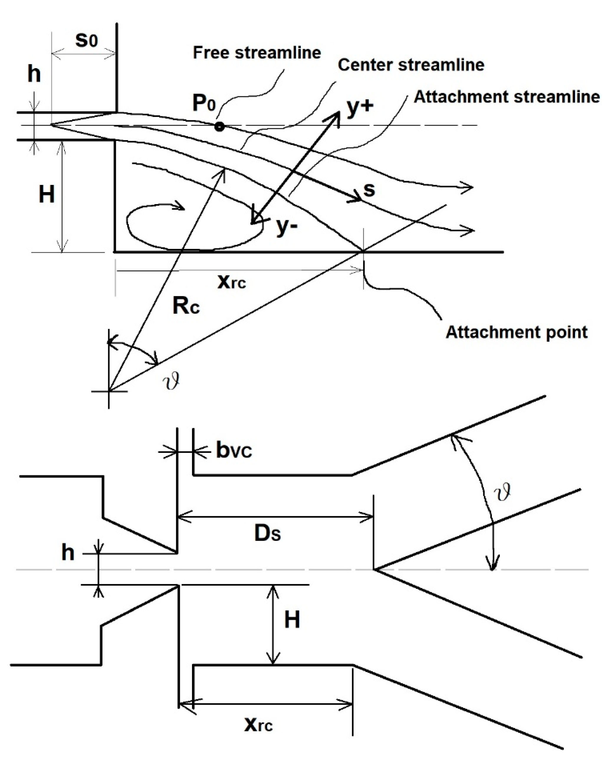
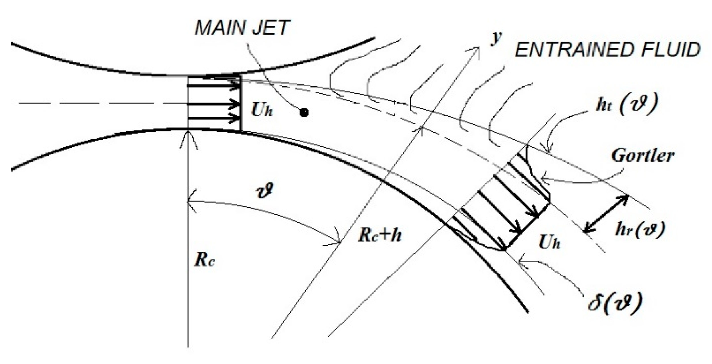
The first target of this study is to characterize the geometric profile of the “Coanda-Diverter” linked to its main fluid dynamics parameters, such as the volumetric flow. To do this the Coanda effect needs to be understood and modeled. In Figure 2 a sketch for the ABD device is reported and used as reference to model the fluid effects. This modeling scheme has been inspired by the one adopted by Hunter in his patent [5], because of the proven simplicity and complete description of all the variables taking part into the mathematical modeling. In the Coanda-Diverter the main inlet flow accelerates in the convergent and flows out the nozzle and (as in the simplified single step case of Figure 2 with closed recirculating zone) finds a lower pressure. This low-pressure field slightly deviates the flow direction from the original straight line to a curved trajectory. The low-pressure region associated to the flow recirculation is a stable structure; it produces the stream attachment to the flow with the so called “first specie Coanda effect”. The configuration of Figure 2 differs from the one of Figure 1 because of the absence of the cusp region, this particular simplification of the geometric model was intended to obtain a better stability of the diverted jet and a “cleaner” design, which is an essential characteristic in order that the apparatus can work with medical or food fluids. Taking into account the above flow structure with the stable recirculation zone, a theoretical model can be developed with the hypothesis of two-dimensional incompressible flow. Considering the theories and analysis from Sawyer, Bourque, Nozaki and Nasr [2,3,6], the relations between the geometry and the flow structure can be obtained with special attention to the distance of the re-attaching point and the radius of the curved stream. Defining as offset ratio the quantity:

$$\mathrm{Offset} \mathrm{ratio}= O_r= \raisebox{1ex}{$H$}\!\left/ \!\raisebox{-1ex}{$h$}\right.>1$$

(3)

The following empirical formulation has been developed by previous authors [2,3]:

$$\frac{x_r}{h}=3.51{\left(\frac{H}{h-1}\right)}^{0.754}$$

(4)

It is valid for $R{e}_h$ in the range 2 × 10⁴–7 ×10⁴ [6]. The Equation (4) denotes the close relation between the re-attaching distance and the off-set ratio defined above. The flow structure, in the specified operating condition interval, depends only on the system geometry. Awbi [7] verified that the flow re-attachment takes place only if the offset distance H is less or equal than a critical height $H_C$ defined as [7]:

$$H_c=6\times \sqrt{\delta h}$$

(5)

where δ is the channel width and $U_0$ is the flow velocity at the nozzle section S. The distance $x_r$ of flow reattachment for the lower streamline depends also on the wall angle. Nasr demonstrated that it increases if the inclination angle increases [8]. In the configuration developed, the wall angle is fixed to zero. Assuming that the radius $R_C$ of the inner streamline is constant and that the curvature arc is tangent to the nozzle axis, a geometrical model can be developed to describe the jet flow characteristic. The velocity profile of the curved jet, symmetrical with respect to the mean streamline, is given by the Goertler equation:

$$U= U_h\times \sec h^2\left(\frac{\sigma y}{s_i}\right)$$

(6)

The equation of the momentum flux represents a crucial step in the mathematical modeling of the problem, as explained by Wada et al. [9]; it allows the momentum balance in the control volume, or the core region of the ABD. The equation is written as follows:

$$J=\rho \underset{-\infty }{\overset{+\infty }{\int }}\left(U^{2}y\right)dy= \frac{4}{3}\rho (U_{\max }^2)\frac{s_i}{\sigma }$$

(7)

where $s_i$ is the curvilinear coordinate along the streamline, y is the radial coordinate and σ is a non-dimensional coefficient known as Spreading Parameter, which expresses the jet opening during flow curvature. Assuming that the Spreading Factor is in the range 40–100 (based on the experience gained on the configuration under study), for the Equation (7) it can be obtained that the maximum jet velocity is:

$$U_{\max }=\sqrt{\frac{3\sigma J}{4\rho s_i}}$$

(8)

Combining the integral expression of the volumetric flow:

$$\dot{Q}=2{\int }_0^{y}Udy$$

(9)

with the flow at the nozzle section ${\dot{Q}}_h=U_{\max }\times h$, one obtains:

$$\underset{0}{\overset{\infty }{\int }}\left(\sqrt{\frac{3\sigma J}{4\rho s_i}}\right)\sec h^2\left(\frac{\sigma y}{s_i}\right)dy=\frac{U_{\max }\times h}{2}$$

(10)

Substituting $s_i=s+s_0$ in this last equation and integrating it, with tanh(0) = 0, it brings:

$$\sqrt{\frac{3J\left(s+s_0\right)}{4\rho \sigma }} = \frac{U_{\max }\times h}{2}$$

(11)

Since $J=\rho U_{\max }^{2}h$ from Equation (11) the expression that relates the position of the virtual origin $s_0$ to the Spreading parameter can be obtained together with the height of the nozzle section:

$$s_0=\raisebox{1ex}{$\sigma h$}\!\left/ \!\raisebox{-1ex}{$3$}\right.$$

(12)

The virtual origin of the jet is the coordinate, measured backwards with respect to the flow velocity from the nozzle section (the enlargement rate of the jet modeled by the coefficient σ is considered linear). With a given value of σ, the position of $s_0$ is obtained. The Spreading factor is an empirical number and no correlations exist to predict it. An iterative calculation is therefore required starting with a first guess as suggested by Chen [10], and then iterate with successive approximations. 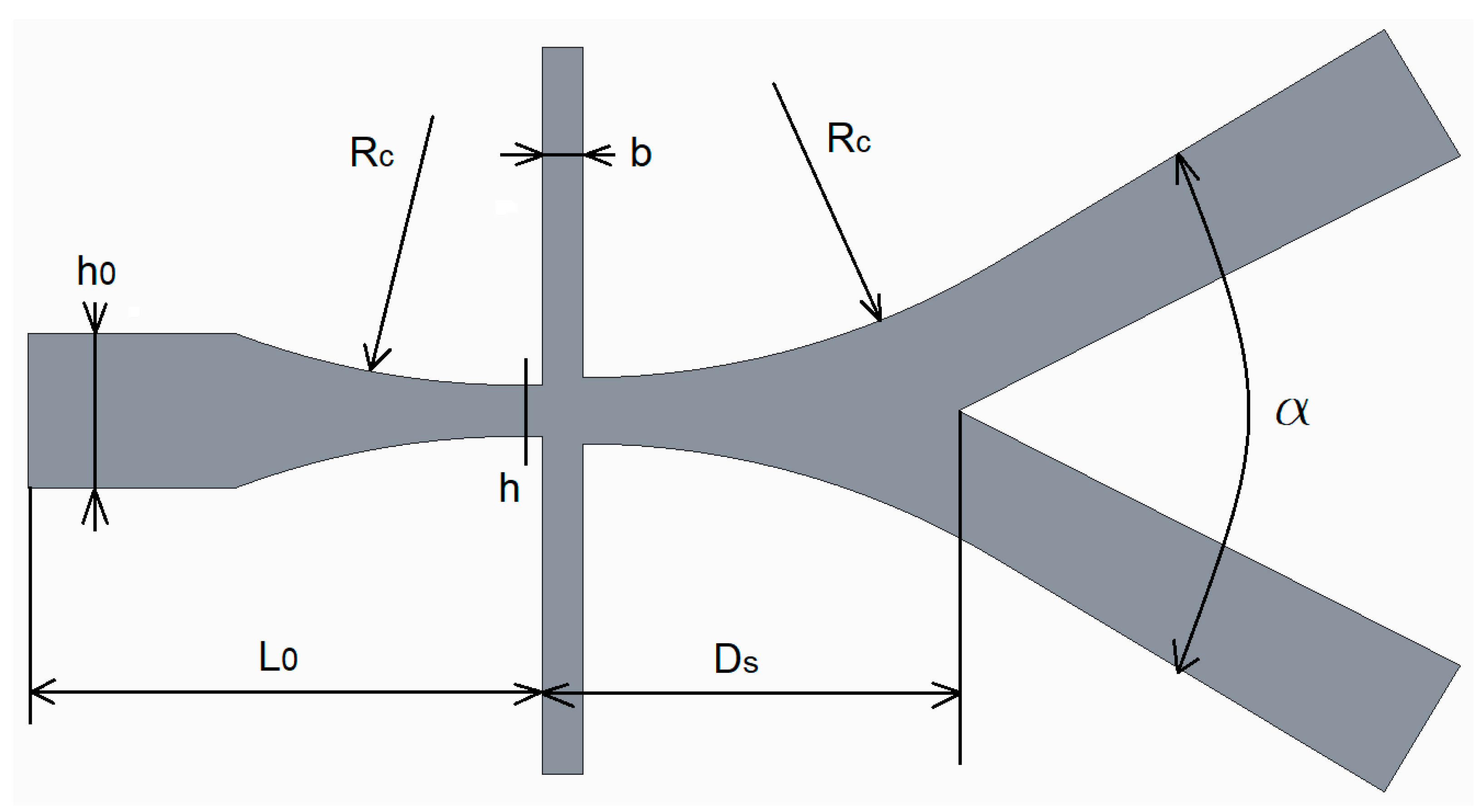The virtual origin coordinate $s_0$ is very important for the dimensioning of the geometrical profile because it allows to correctly compute the value of the distance $D_S$ (Figure 3 and Figure 4) to avoid interference with the jet itself. The so called “enhancement coefficient” $C_a$, can be computed or, equivalently, the tangent of the angle between the external layer line and the horizontal plane:

$$C_a=\frac{h/2}{s_0}=\frac{h}{2s_0}=\frac{3}{2\sigma }$$

(13)

Since the curvilinear position s can be expressed in polar coordinate $s=R_c\ast \theta$, the following trigonometric equation can be written to calculate the height of the curved jet as a function of the center angle θ:

$$h\left(s\right)=h+\left(C_a\times s\right)$$

(14)

With the introduction of the relation for the coordinate s and the equation for the jet height $h^{*}$ at the angle ${\theta }^{*}$ (which locate the point $P_o$) it becomes:

$$h^{*}=h+\left(C_a{R}_c{\theta }^{*}\right)$$

(15)

The following system with the three unknowns $x_{P0}$, ${\theta }^{*}$ and $h^{*}$ is obtained:

$$\{\begin{array}{c}\left(R_c+h^{*}\right)\sin {\theta }^{*}=x_{P0}\\ \left(R_c+h^{*}\right)\cos {\theta }^{*}=R_c+\frac{h}{2}\end{array}$$

(16)

After substitution of Equation (15), it becomes:

$$\{\begin{array}{c}\left[R_c+h+\left(C_a{R}_c{\theta }^{*}\right)\right]\sin {\theta }^{*}=x_{P0}\\ \left[R_c+h+\left(C_a{R}_c{\theta }^{*}\right)\right]\cos {\theta }^{*}=R_c+\frac{h}{2}\end{array}$$

(17)

The above system (17) can be solved numerically, taking into account that the angle ${\theta }^{*}$ will be realistically in the range 0–45°. After a revision of the available literature for similar configurations [11,12,13,14], a first geometry guess for the ABD is obtained assuming the parameters in

Table 1. Reference values for the standard geometry.

Off-Set Ratio	Nozzle Height	Nozzle Cross-Section	Spreading Factor	Divergence Angle for the Discharge Channels	Apparatus Thickness
2.125 mm	2 mm	4 ${\mathrm{mm}}^2$	50	6°	2 mm

.

The flow attachment point coordinate is:

$$x_r=h\times 3.51{\left(\frac{H}{h-1}\right)}^{0.754}$$

and the curvature radius and the deviation angle are:

$$\{\begin{array}{c}{R}_c\sin \left(\alpha /2\right)=x_r\\ R_c\cos \left(\alpha /2\right)=R_c-h\end{array}\Rightarrow \{\begin{array}{c}{R}_c\\ \alpha \end{array}$$

Finally, ${\theta }^{*}$ and $x_{P0}$ are obtained from the system (17). With the value of the off-set ratio, a value of the off-set height H high enough to satisfy the Awbi’s criteria for the attachment can be obtained:

$$H_{\mathrm{crit}}>H$$

All the main profile dimensions have been obtained and the device geometry can be parameterized with respect to the nozzle height h, as reported in

Table 2. Parametrization of the ABD’s geometry.

Symbol	Parametric Value
h	2 mm
Rc	25 mm
Ds	12 mm
b	1.25 mm
$h_0$	3 mm
γ	10°
l	$2 \mathrm{mm}$

, where $C_n$ are the computed coefficient. This parametrization criterion for the geometry was conceived because h defines the area of the nozzle cross-section and so the volumetric flow evolving in the ABD; h defines the “size” of the apparatus. The evolving fluid is water and cavitation could be an issue. It is therefore necessary to check if the local flow pressure goes below the vapor pressure.

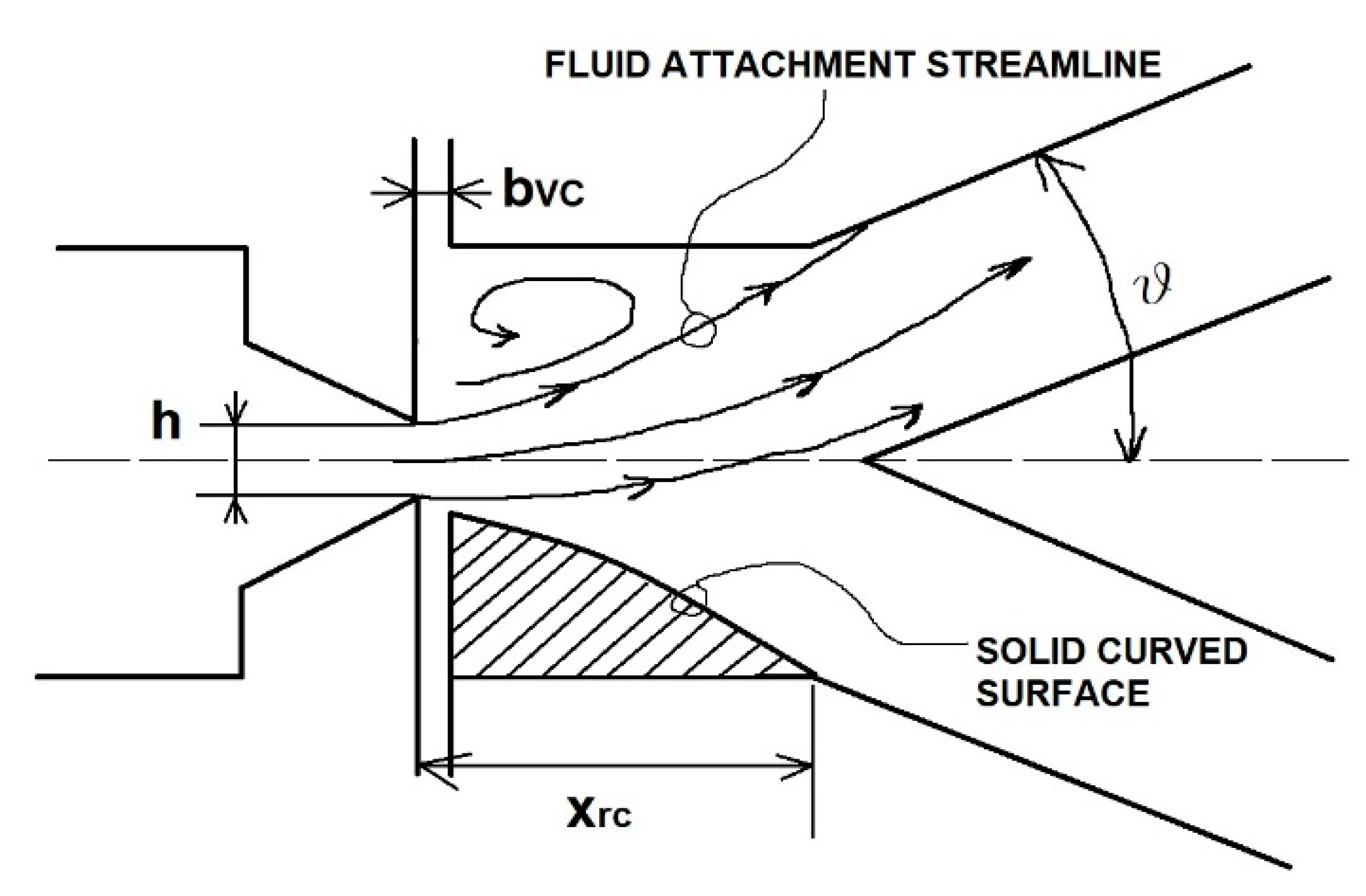
In the device configuration of Figure 2 the presence of cavitation risk has been highlighted with CFD analysis and experimental tests. To avoid the problem, the geometric profile of the ABD is coincident with the flow channel obtained by the limiting streamlines. In this way, the sharp steps where the recirculation zones develop are substituted by the lower flow streamline profile having a circular form. In Figure 3 the flow recirculation zone is replaced with its physical equivalent; the recirculation bubble is excluded and a new geometrical configuration is obtained as detailed in Figure 4. In the improved design, the Coanda effect takes place not because of the pressure differential between the upper zone of the jet and the recirculation bubble, but due to the pressure differential inside the jet itself, created by the skin friction through jet and the solid convex nearby wall.

3. Mathematical Model of the ABD

In Figure 5, a sketch of the configuration under study is reported and the mathematical model is based on this reference flow structure

The following hypothesis have been made, also considering the mathematical modeling of similar problems made for example by Patterson [15]:

(a)

The flow is steady, two-dimensional and incompressible.

(b)

The velocity profile at the nozzle section is uniform.

(c)

The decrease in maximum jet speed along the surface is considered negligible, because of the low deviation angle.

(d)

The cylindrical surface center angle occupied by the submerged flow is θ* and this portion of the jet is associated to the external entrainment.

(e)

The velocity profile of the curved jet is given by Gortler Equation (6).

It holds:

$$h\left(\theta \right)=h+\left[C_a\ast \left(R_c\theta \right)\right]$$

(18)

with the Equation (13) it follows:

$$h_r\left(\theta \right)=C_a\ast \left(R_c\theta \right)=\frac{3R_c\theta }{2\sigma }$$

(19)

The above gives the dependence between the entrainment portion of jet height and the center angle θ. Using the velocity profile from Equation (6), it is possible to compute the amount of aspirated flow from the passive channel. Starting from the integral expression of the volumetric flow:

$${\dot{Q}}_y=\underset{0}{\overset{y}{\int }}Udy= \underset{0}{\overset{y}{\int }}\left[U_h\sec h^2\left(\frac{\sigma y}{s_i}\right)\right]dy$$

(20)

It follows:

$${\dot{Q}}_y=U_h\tan h\left(\frac{\sigma y}{s_i}\right)$$

(21)

Making the following substitution:

$$\begin{array}{c}y=h_r\left({\theta }^{*}\right)=C_a{R}_c{\theta }^{*}=h_r^{*}\\ s_i=s_0+s^{*}\end{array}$$

(22)

where:

$$s^{*}=\left(R_c+\frac{h}{2}\right){\theta }^{*}$$

(23)

and the angle θ* given by the system of Equation (17):

$$\{\begin{array}{c}(R_c+h_r^{*})\cos {\theta }^{*}=\left(R_c+\frac{h}{2}\right)\\ (R_c+h_r^{*})\sin {\theta }^{*}=D_s\end{array}\stackrel{\mathrm{yields}}{\to }\tan {\theta }^{*}=\left(\frac{2D_s}{2R_c+h}\right)$$

a relevant expression for the volumetric aspired flow ${\dot{Q}}_r$ is obtained in the following Equation (24):

$${\dot{Q}}_r=l{U}_h\left\{\tan h\left[\frac{9}{2}\frac{R_c{\tan }^{-1}\left(\frac{2D_s}{2R_c+h}\right)}{\sigma h+3\left(\left(R_c+\frac{h}{2}\right){\tan }^{-1}\left(\frac{2D_s}{2R_c+h}\right)\right)}\right]\right\}$$

(24)

${\dot{Q}}_r=f\left(l,R_c,D_s,h,\sigma ,U_h\right)$ correlates the volumetric flow to the geometric parameters of the ABD profile. The product $l{U}_h$ can be written as a function of the Reynolds number at the nozzle cross-section, to get a more interesting form of the previous form, as in the following Equation (25):

$${\dot{Q}}_r=R{e}_h\nu \frac{l}{h}\left\{\tan h\left[\frac{9}{2}\frac{R_c{\tan }^{-1}\left(\frac{2D_s}{2R_c+h}\right)}{\sigma h+3\left(\left(R_c+\frac{h}{2}\right){\tan }^{-1}\left(\frac{2D_s}{2R_c+h}\right)\right)}\right]\right\}$$

(25)

where the relevant geometric parameter l/h (aspect ratio) is introduced. This is the target expression for the passive volumetric flow in the ABD; it gives the relation between a characteristic operative parameter and the geometric profile of the apparatus, so it directly correlates the ABD fluid dynamics to its geometry. The fluidic performance in terms of velocity ratio at a given section or pressure ratio are independent on the flow rate. The spreading parameter σ in Equation (25) can be used as tuning parameter to properly adjust the analytical model to a given geometry, as suggested by Chen [10]. A non-dimensional characteristic number for the ABD to represent the inlet volumetric flow fraction that is entrained and aspired from the passive outlet can be introduced. This is called Drag Coefficient Ω. The inlet flow can be computed with:

$${\dot{Q}}_{\mathrm{in}}=S_0{U}_0=(l{h}_0)\sqrt{2\frac{\left(p_{\mathrm{in}}-p_{\mathrm{out}}\right)}{\rho }}$$

(26)

Considering Equation (25), Ω is obtained with the following Equation (27):

$$\Omega =\frac{{\dot{Q}}_r}{{\dot{Q}}_{\mathrm{in}}}=\frac{1}{h}\left\{\tan h\left[\frac{9}{2}\frac{R_c{\tan }^{-1}\left(\frac{2D_s}{2R_c+h}\right)}{\sigma h+3\left(\left(R_c+\frac{h}{2}\right){\tan }^{-1}\left(\frac{2D_s}{2R_c+h}\right)\right)}\right]\right\}$$

(27)

The parameter Ω depends only on the configuration geometry and the discharged flow can be therefore computed with:

$${\dot{Q}}_{\mathrm{out}}=\left(\Omega {\dot{Q}}_{\mathrm{in}}+{\dot{Q}}_{\mathrm{in}}\right)={\dot{Q}}_{\mathrm{in}}\left(\Omega +1\right)$$

(28)

The following considerations can be drawn:

• with a Reynolds number increase, the inlet flow amount grows, this increases both suction and discharge flows. At higher inlet pressures an increase of the passive flow is expected, but, from Equation (27), the ratio Ω remains the same;
• to increase the effective mass flow with a given differential pressure (difference between inlet and outlet) the cross-section area is increased (by increasing the width l) but this will also raise the passive flow linearly;
• the $h_0/h$, ratio has no influence on the net elaborated flow. With a fixed width l a higher h increases both inlet and outlet flows.

With the use of CFD a correlation for the inlet volumetric flow can be obtained, as showed in Figure 6. The above function takes into account all the pressure losses due to the viscous flow and flow non-uniformities. The following loss coefficient can be introduced:

$$\Psi =\frac{U_{0 \mathrm{real}}}{U_{0 \mathrm{ideal}}}=\frac{U_{0 \mathrm{real}}}{\sqrt{2\frac{\left(p_{\mathrm{in}}-p_{\mathrm{out}}\right)}{\rho }}}$$

(29)

The following correlation has been developed with respect to the inlet pressure:

$$\Psi \left(p_{\mathrm{in}}\right)=\left[4+5.8p_{\mathrm{in}}-0.48{\left(p_{\mathrm{in}}\right)}^2\right]\ast {\left[2\frac{\left(p_{\mathrm{in}}-p_{\mathrm{out}}\right)}{\rho }\right]}^{-\frac{1}{2}}$$

(30)

A further step in the model development is the prediction of the boundary layer inside the channels. The exponential velocity profile for a turbulent boundary layer from Schlitching [16] is considered:

$$\frac{U}{U_{\infty }}={\left(\frac{y}{\delta }\right)}^{1/n}$$

(31)

and n = 7 allows good results for the Coanda effect at the wall, as supported also by the work of Pope and Pelfrey [17,18] for the mathematical modeling of generalized turbulent flows, with particular reference to the flat plane flow equations and the turbulent curved jets, as reports Trancossi [19]. Trancossi [11] demonstrated that with the hypothesis of moderate wall curvature (i.e., the curvature ratio $C_r=\raisebox{1ex}{$h$}\!\left/ \!\raisebox{-1ex}{$R_c$}\right.\ll 1$) the boundary layer analysis is close to the flat plate case. So, defining a proper Reynolds number, relative to the outflow on the convex wall:

$$R{e}_x=\frac{U_{\infty }x}{\nu }=R{e}_s=\frac{U_h{R}_c\theta }{\nu }$$

(32)

the development of the boundary layer thickness δ along the x coordinate and the skin friction coefficient c_f are:

$$\frac{\delta }{x}=0.166\left(R{e}_s^{-1/7}\right)$$

(33)

$$c_f=0.0277\left(R{e}_s^{-1/7}\right)$$

(34)

Therefore, the wall stress:

$${\tau }_w=0.01385\left(R{e}_s^{-1/7}\right)\times \rho \times U_h^2$$

(35)

and the expression of the stress-tangential velocity u_τ follows:

$$u_{\tau }=\sqrt{\frac{{\tau }_w}{\rho }}\cong 0.1354\left(R{e}_s^{-\frac{1}{14}}\right)U_h$$

(36)

The above Equation (36) can be taken as the amount of flow velocity lost because of the skin friction at the walls. This is very important for the Coanda effect, which takes advantage from the pressure gradient inside the jet, or along the curvature radius, due to the wall stress. The above model can also be used to calibrate the meshing parameters in the CFD model. From Equation (33) the relevant expression of the boundary layer thickness along the curved wall is obtained (37):

$$\delta \left(x\right)=0.166x\left(R{e}_s^{-1/7}\right) \to \delta \left(\theta \right)=0.166\left(R_c\theta \right)\left(R{e}_s^{-1/7}\right)$$

(37)

The development is directly proportional to the x-coordinate along the wall, which is given by $x=R_C\theta$. This is coherent with both the experimental observations of Englar’s work [20] and the mathematical modeling of the Coanda effect proposed by Franzulica [21], which relates the growth rate of the boundary-layer on the curved wall directly to the angle θ, so to the coordinate x, as also supported by Kind and Benner [22,23]. The ABD fluid domain is divided into three main fluid regions: Zone-I represents the inlet convergent; Zone-II the deviation convex walls and Zone-III is the active discharge channel. For the zones I and III the equations of the boundary layer for confined flow can be used:

$${\tau }_w=0.03955\rho {(\overline{u})}^{-\frac{7}{4}} {\nu }^{\frac{1}{4}}{d}^{-\frac{1}{4}}$$

(38)

and:

$$u_{\tau }=\sqrt{\raisebox{1ex}{${\tau }_w$}\!\left/ \!\raisebox{-1ex}{$\rho $}\right.}=0.1989{\overline{u}}^{\left(-\frac{7}{8}\right)}{\nu }^{1/8}{d}^{\left(-\frac{1}{8}\right)}$$

(39)

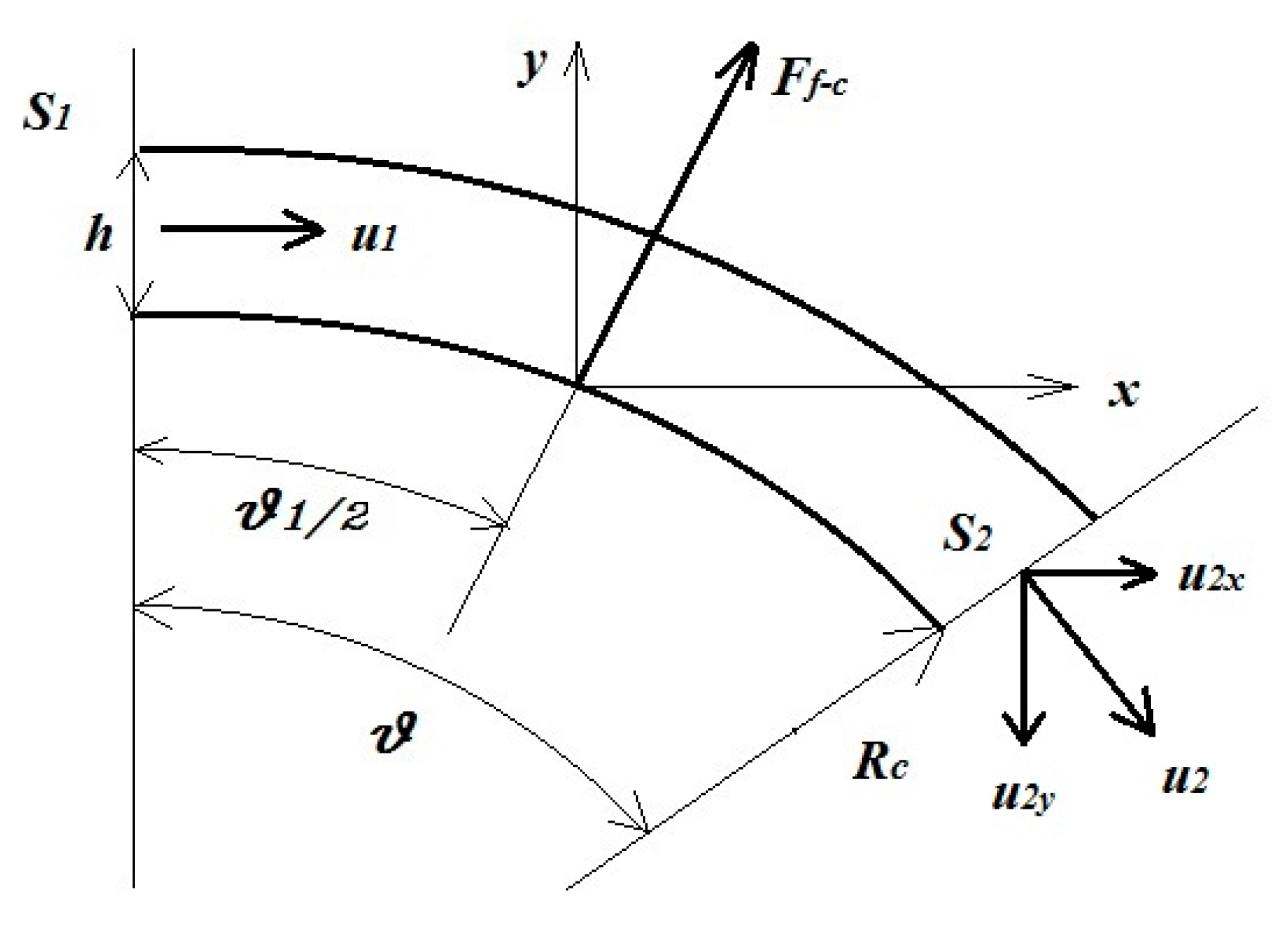
The wall stresses for the three zones can be therefore computed with a given flow regime. In the present case in the Zone-I the wall stress magnitude is 1 × 10⁴ N/mm², while in the Zone-II is 1 × ${10}^3$ N/mm². To complete the theoretical model of the apparatus, forces acting on the flow can be computed from the conservation of momentum. In the axial direction in the convergent:

$$F_{x \mathrm{conv}}=\rho \left(l{h}_0{\left(\frac{Q_{\mathrm{in}}}{h_0\delta }\right)}^2-lh{\left(\frac{Q_{\mathrm{in}}}{lh}\right)}^2\right)=\rho l{Q}_{\mathrm{in}}^2\left(\frac{1}{h_0}-\frac{1}{h}\right)$$

(40)

The axial and tangential components due to the flow curvature, referring to Figure 7:

$$F_x=\rho lh{\left(\frac{Q_{\mathrm{in}}}{h\delta }\right)}^2-\rho lh{\left(\frac{Q_{\mathrm{in}}}{h\delta }\cos \theta \right)}^2=\rho \frac{Q_{\mathrm{in}}^2}{lh}\left(1-{\cos }^2\theta \right)$$

(41)

$$F_y=\rho lh{\left(\frac{Q_{\mathrm{in}}}{lh}\sin \theta \right)}^2=\rho \frac{Q_{\mathrm{in}}^2}{lh}{\sin }^2\theta$$

(42)

4. CFD Modeling: Steady Flow

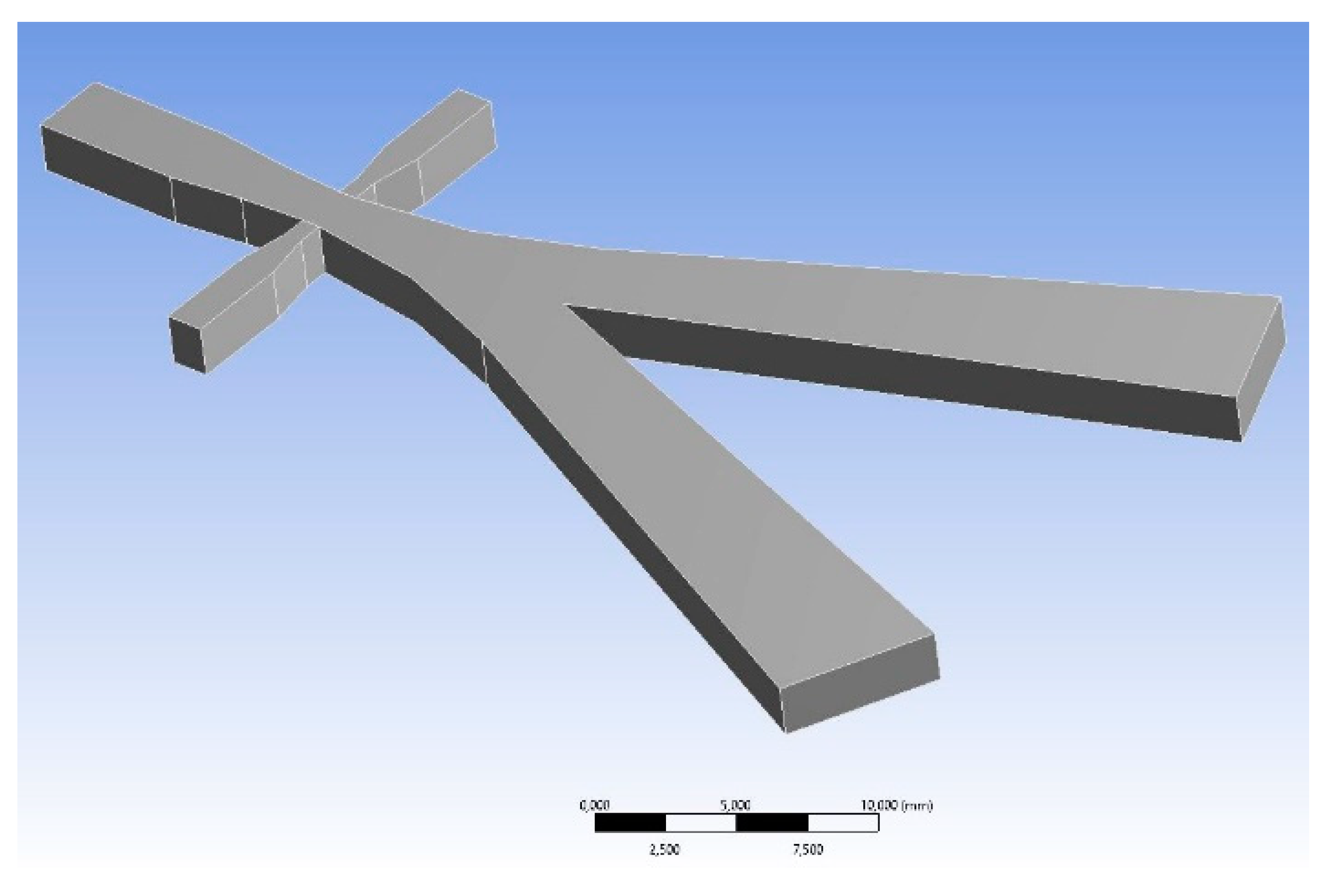
A numerical simulation approach based on CFD has been developed in order to have a further understanding of the flow structure, fluidic performance of the device. The simulation approach has been also used to validate the theoretical design model. The CFD model is based on the commercial software Fluent and both 2D and 3D models are considered. The reference 2D geometry is for the device ABD reported in Figure 4; the three-dimensional cases are obtained by extruding the 2D-case, as shown in Figure 8. Referring to Figure 4 it can be observed that the convergent duct has a particular shape: the first convergent part has straight lines (the fluid gradually accelerates relative to the taper angle) while the second convergent part has curved walls modeled with a circular shape (the fluid gains a pre-rotation effect, which allows the Coanda effect). The simulations are setup with incompressible adiabatic flow and, in this first part, with steady operating condition.

A crucial step for the CFD analysis of this device is the mesh generation. Due to the low energy effects that act at the boundary layer scale and drive the Coanda effect, it is necessary to generate a high quality and fine mesh to solve the boundary layer development. Unstructured mesh is considered. Viscous mesh layers are added and the mesh layers clustering at walls has the following rule:

$$H=\Delta s\times {(Gr)}^{N-1}$$

(43)

where Δs is the first layer thickness, N is the layer number and Gr the growth rate. The mesh clustering at the wall is required to guarantee for non-dimensional distance $y^{+}$ in the boundary layer of the order of one. The value of $y^{+}$:

$$u_{\tau }=\frac{\mu }{\rho }\frac{y^{+}}{\Delta s}$$

(44)

cannot be fixed during the setup phase but needs to be checked after a first simulation. In order to have a reasonable guess for the first grid line distance from the wall the Equation (36) can be used. The growth rate and the number of layers are then fixed in order to get a mesh layer of the order of the boundary layer thickness estimated with Equation (37). Figure 9 shows a view of the mesh with a detail on the viscous mesh layers. The mesh quality is checked using the available parameters in the reference grid generation code.

A global mean quality index of at least 85% is required for the present meshes. The SST turbulence model has been selected for both steady and unsteady analysis. Said model was chosen for its robustness in modeling turbulent flows with separation, as also reported by the work of Wilcox, Launder and Menter [24,25,26], who gives a very detailed description and support on the turbulence modeling in CFD simulations. So a simulation campaign has been performed in order to:

• test the correct working principle and validate the mathematical model;
• obtain the characteristic flow curves for the ABD device.
• predict the switching time and the minimum switching pressure necessary in the actuation channels.

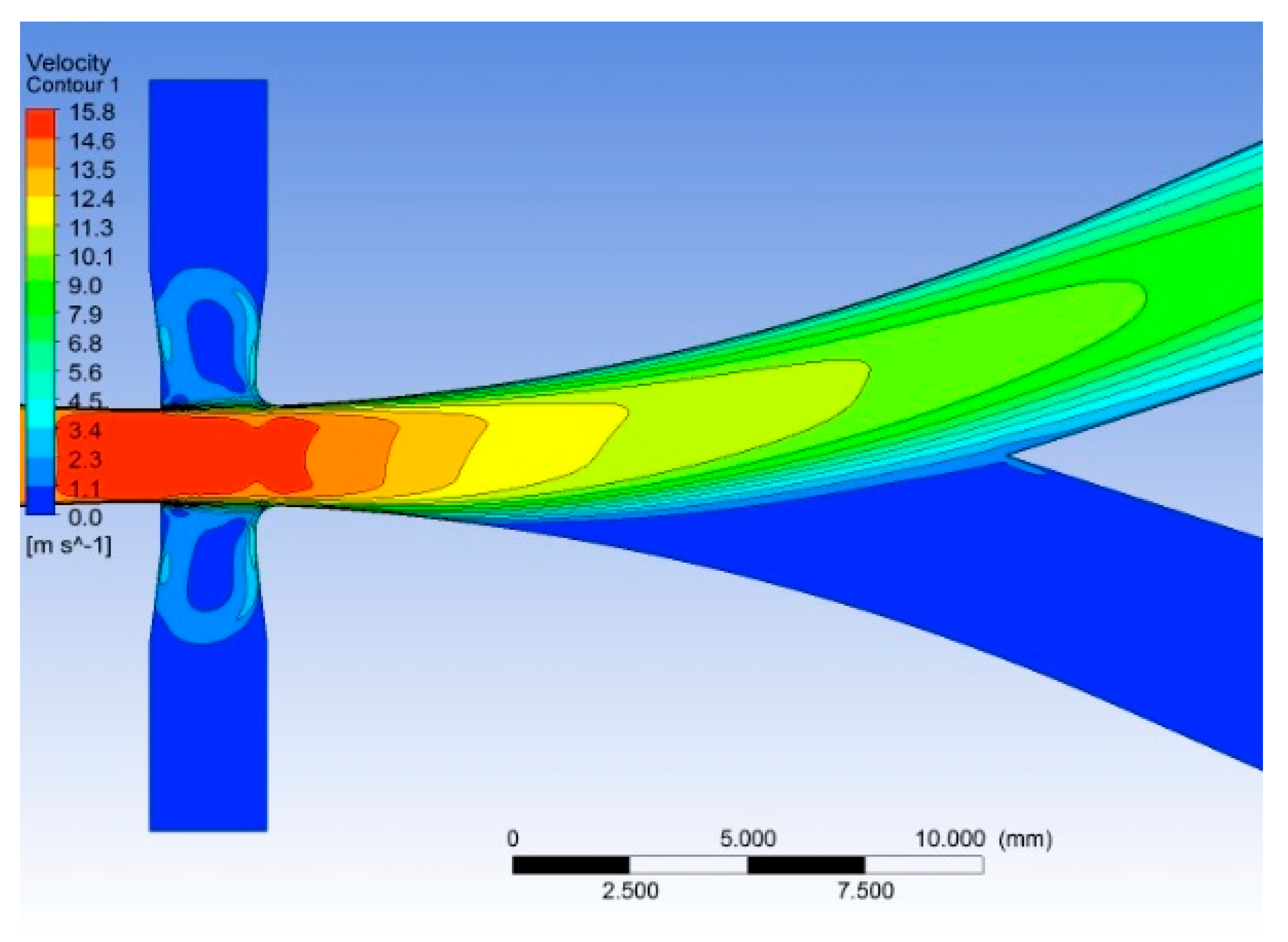
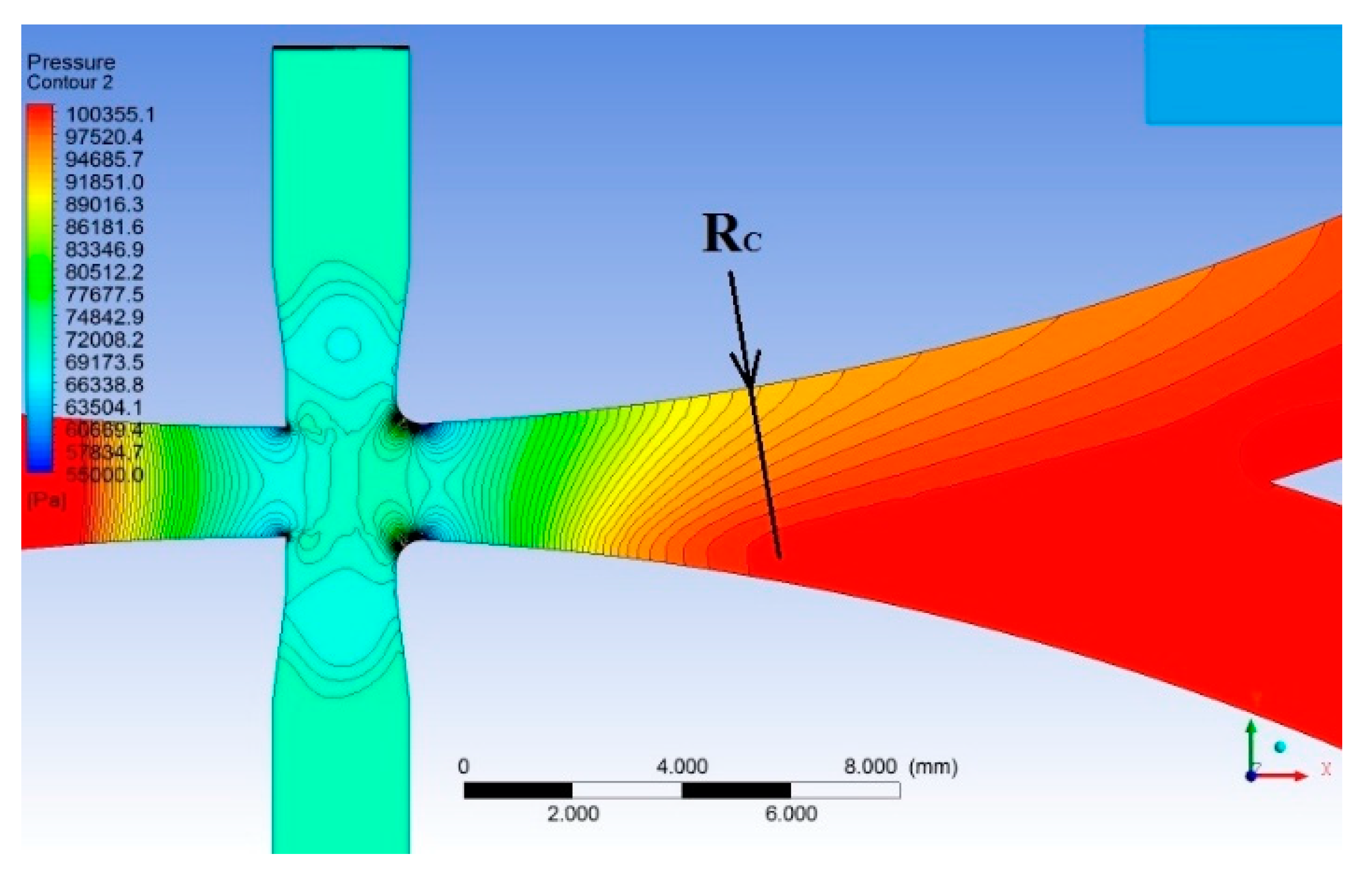
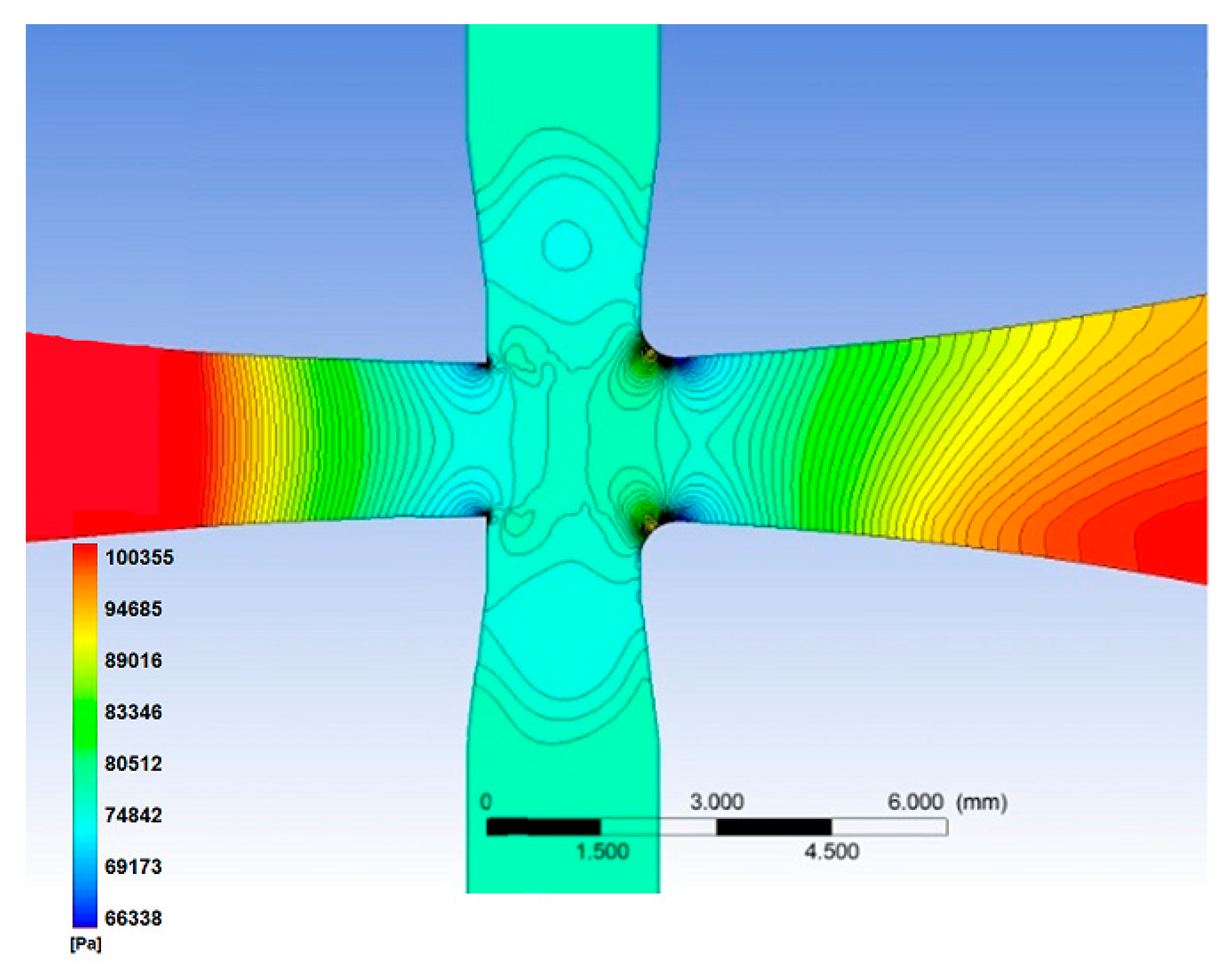
The correct operation of the device has been confirmed. In Figure 10 the wall attachment of the jet is confirmed by the flow velocity contours obtained with an inlet pressure of 1.0 (bar) and both the actuation channels closed. A perfect flow symmetry is obtained in the core region and at the crossing point between inlet and side channels; in this condition the direction of flow deviation can be obtained up or down with the same command signal (pressure perturbation). This aspect is confirmed by the static pressure contours for the same case reported in Figure 11.

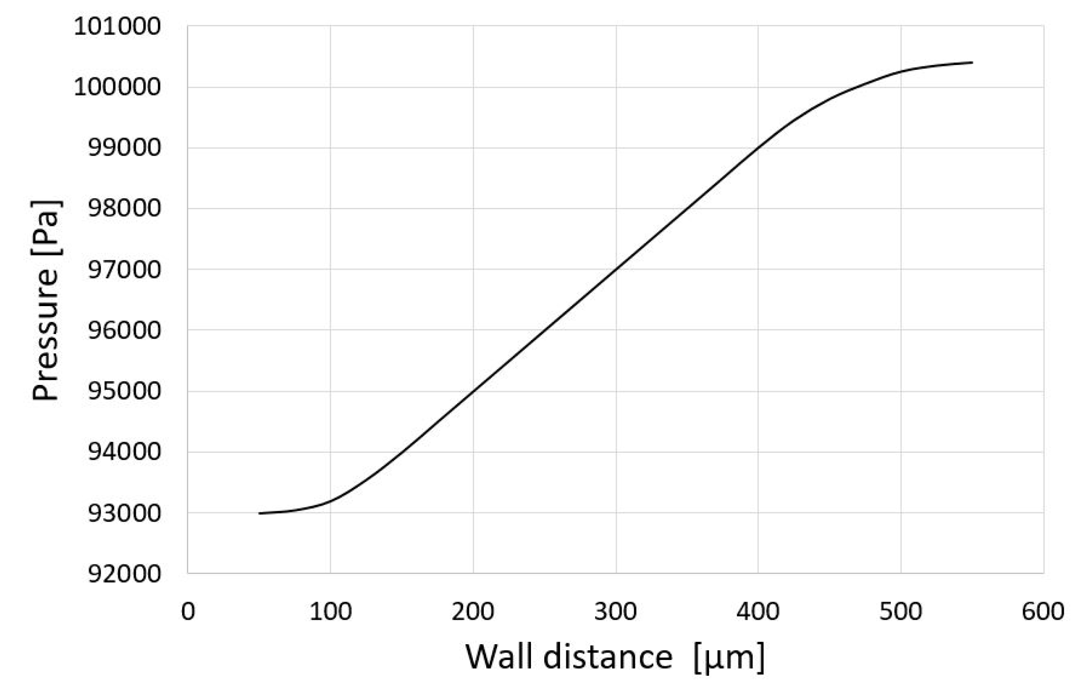
In Figure 12, the pressure distribution along the radial coordinate of the attachment wall is shown. A large zone where linear distribution is obtained and, as expected, the pressure near the wall is lower than outside the jet (atmospheric).

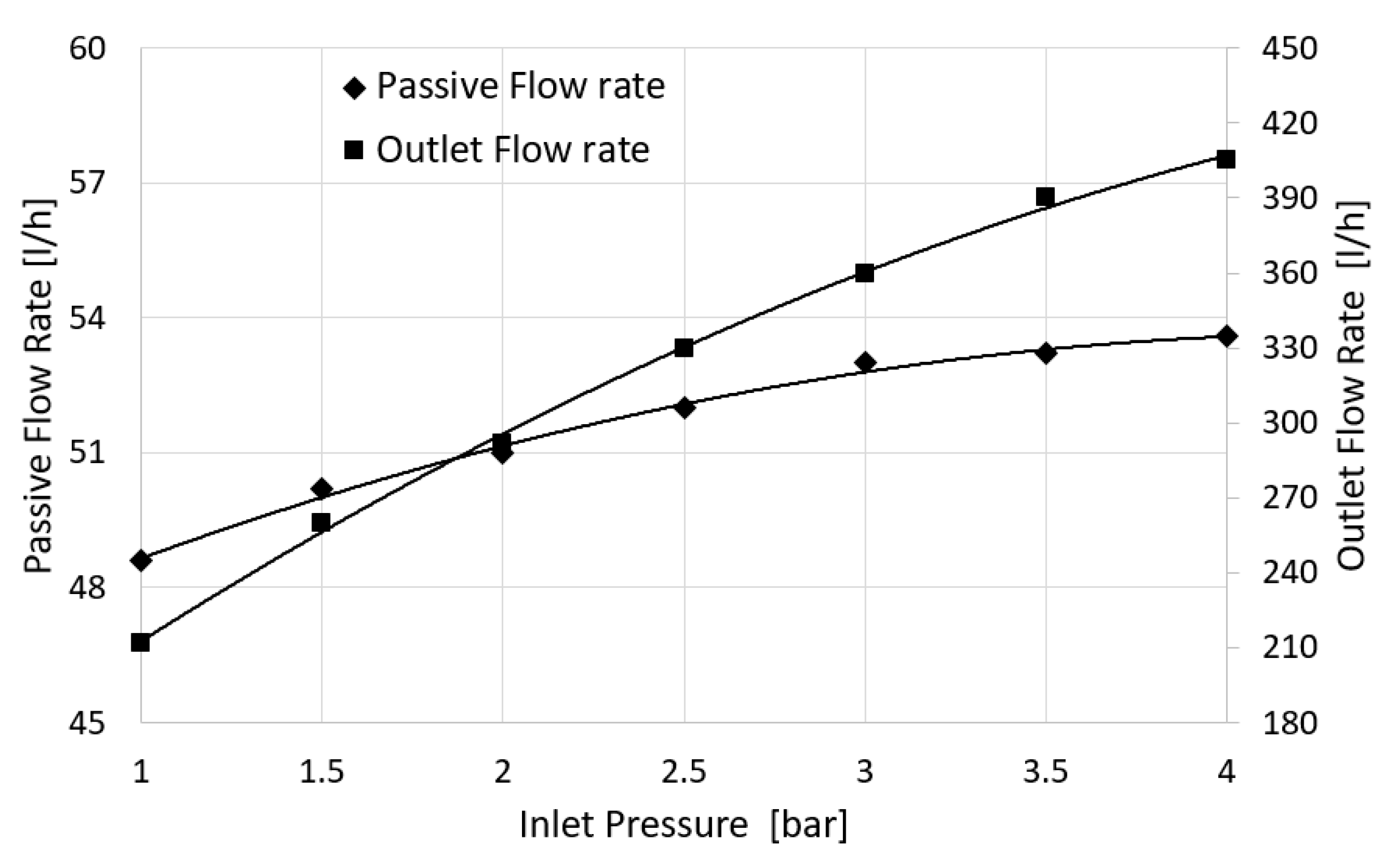
A good accuracy has emerged between the expected and the simulated values for the volumetric flow involved in the ABD steady regime.

Table 3. Volumetric flows comparison: predicted vs. CFD.

Flow	CFD (lph)	Design (lph)	Difference
Inlet	222.76	222.91	+0.067%
Outlet	274.75	274.63	−0.043%
Passive	51.98	51.72	+0.5%

shows the volumetric flow rate for the baseline geometry configuration and an inlet pressure equal to 1 (bar). The difference between the expected values and the CFD results is below 0.5% for the three control sections. The CFD model has been used to obtain the performance curves of the device and to compare them with the reference curves from the theoretical model. 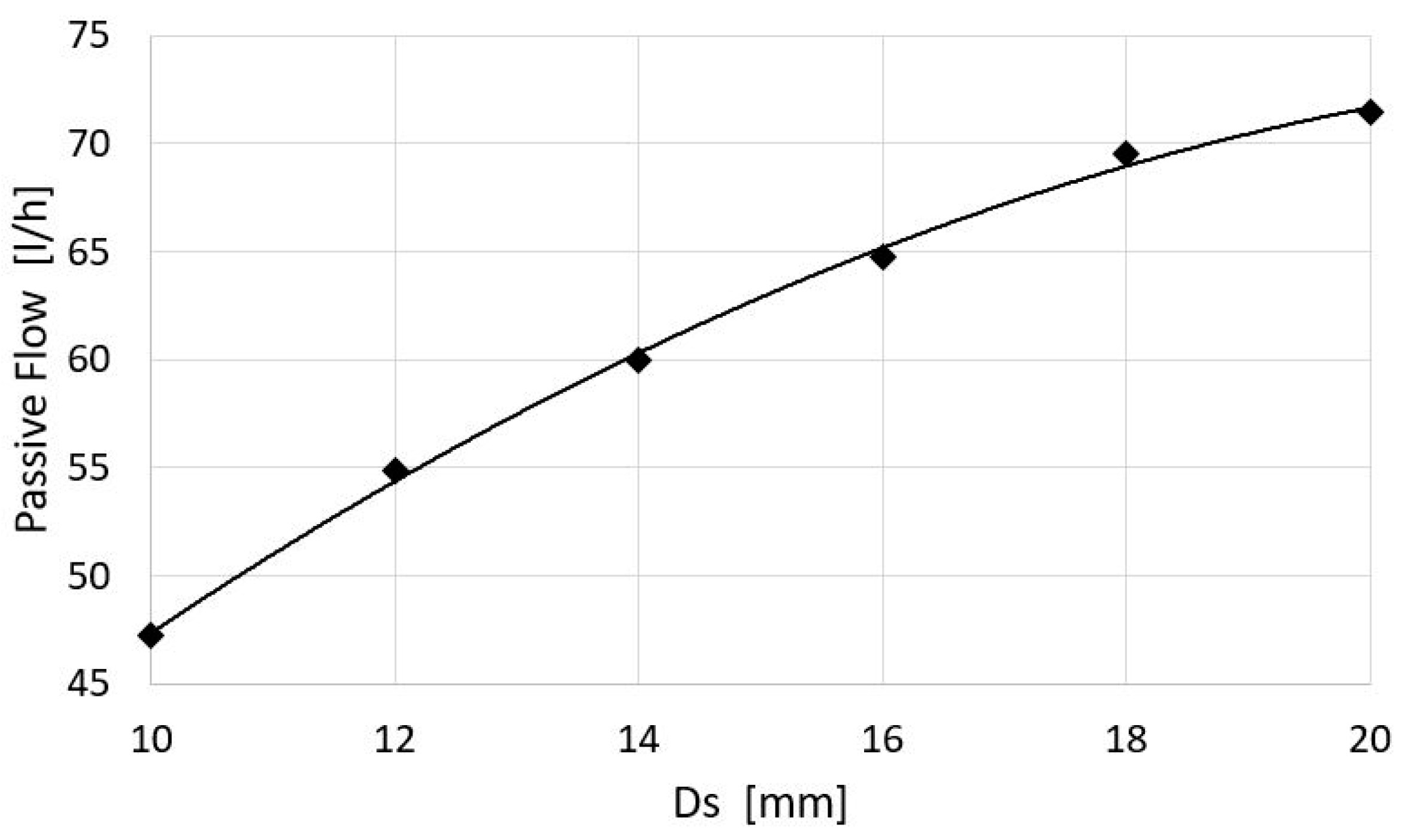A parametric configuration as described in Table 2 has been considered. In Figure 13, the theoretical curve for the passive flow rate with different values of Ds is shown and compared to the CFD analysis (dots); an excellent agreement is obtained.

This can be achieved with the proper choice of the spreading parameter σ that acts as a tuning parameter. Regarding the coefficient Ω, a value of 0.2017 was fixed in the design and a mean value of 0.202 has been obtained with CFD; this is not affected by the inlet flow.

In Figure 14, the passive flow rates from the theoretical model for different geometrical configurations with a change of the septum distance DS are compared to the CFD values (black dots). A good robustness of the theoretical model (Equation (25)) to geometry change is evident from the good matching with the simulated values.

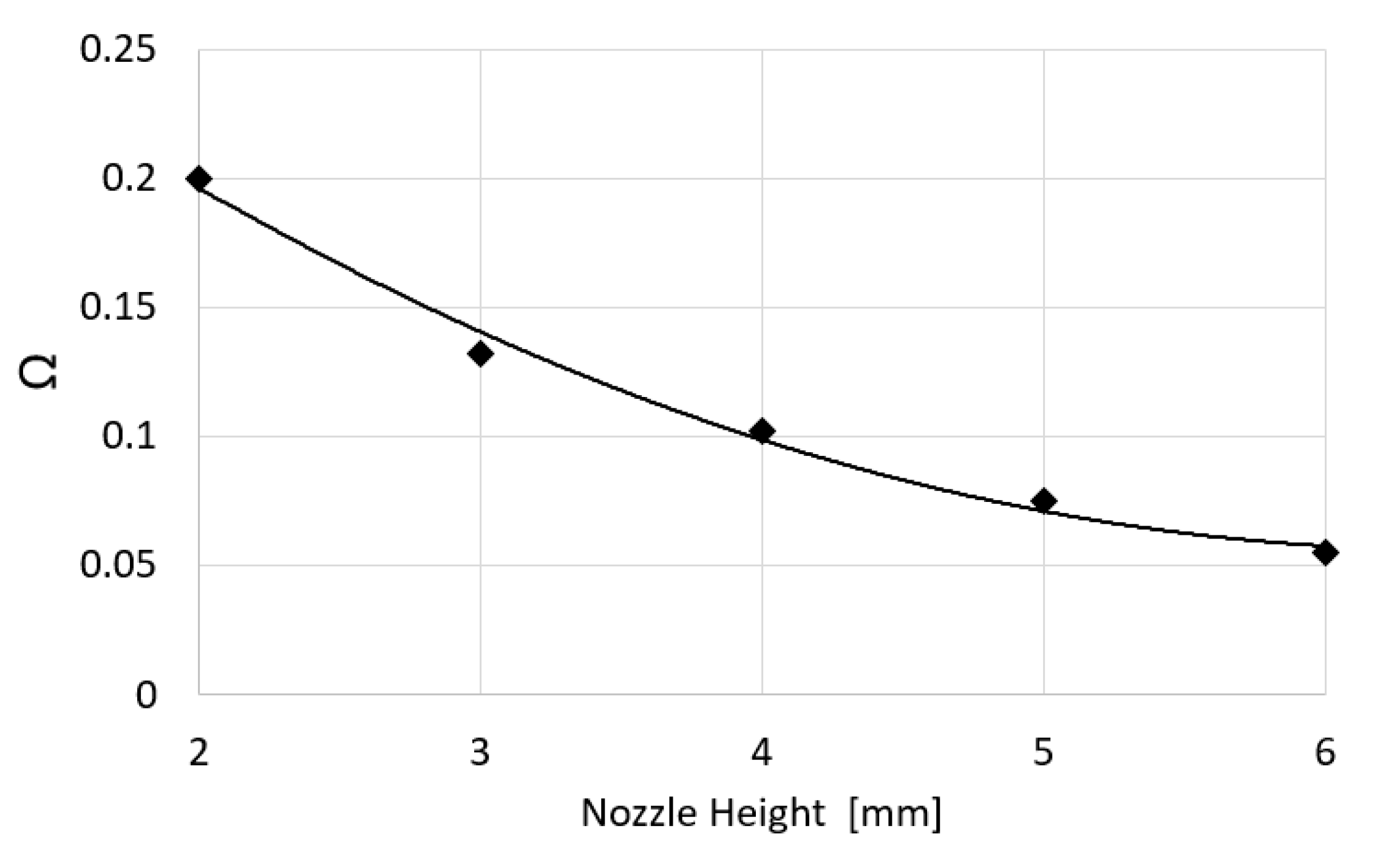
A further comparison and validation of the theoretical model has been done for the relation of the coefficient Ω versus the nozzle height h. In Figure 15, the theoretical curve and the CFD data (dots) are compared. The Ω decreases with growing h because of the inlet section value:

$$S_{in}=h_0\times l=1.5h^2 \Rightarrow {\dot{Q}}_{in}=(S_{in}\times U_{in}) \sim h^2$$

In case of curved flow:

$$S_r \sim \frac{D_s}{h_{jet}}\times l \Rightarrow {\dot{Q}}_r \sim l \Rightarrow {\dot{Q}}_r \sim h$$

A good match between the modeled and simulated values is obtained. The above comparisons confirm the theoretical model as a valid design tool for the device.

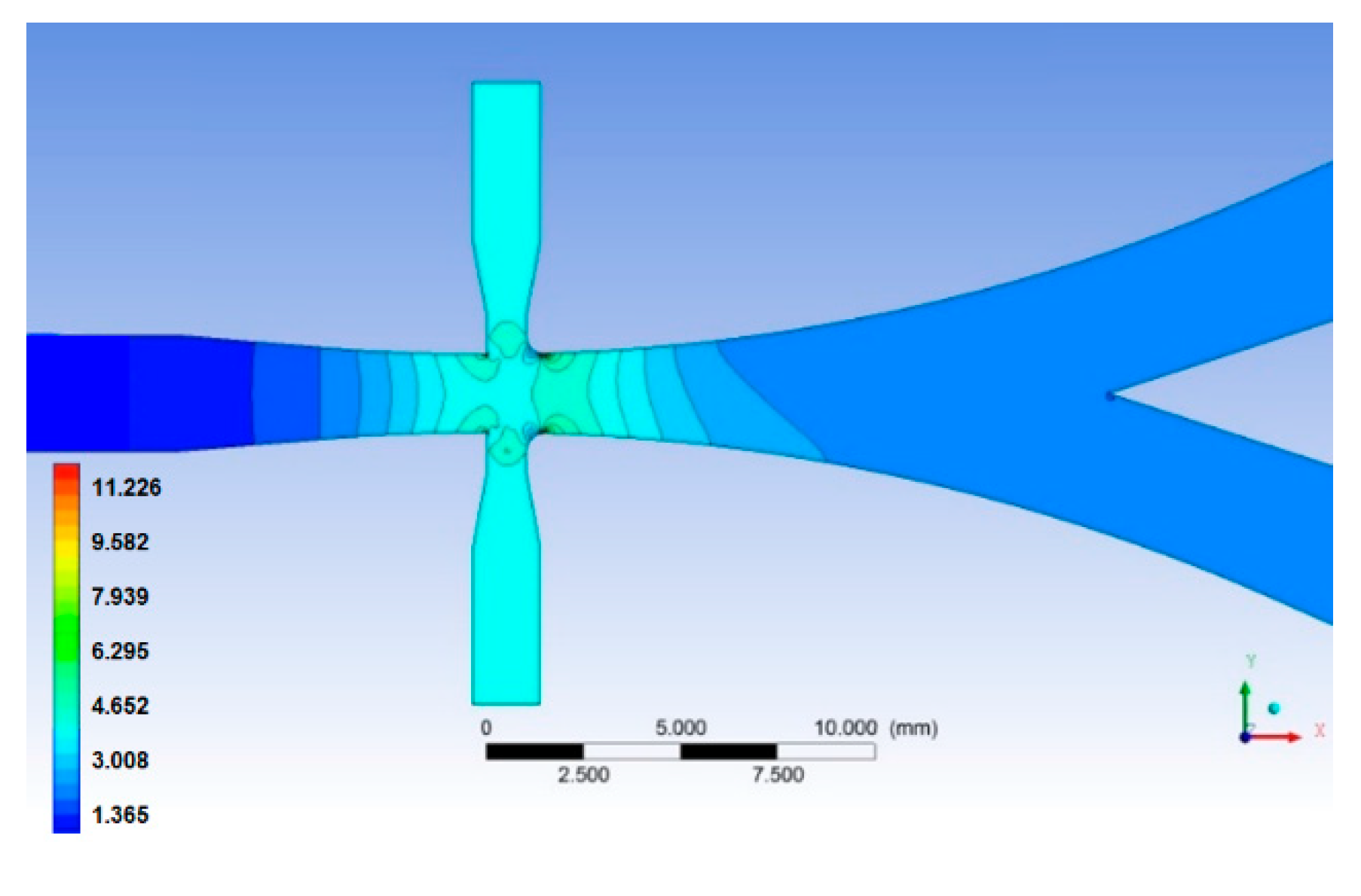
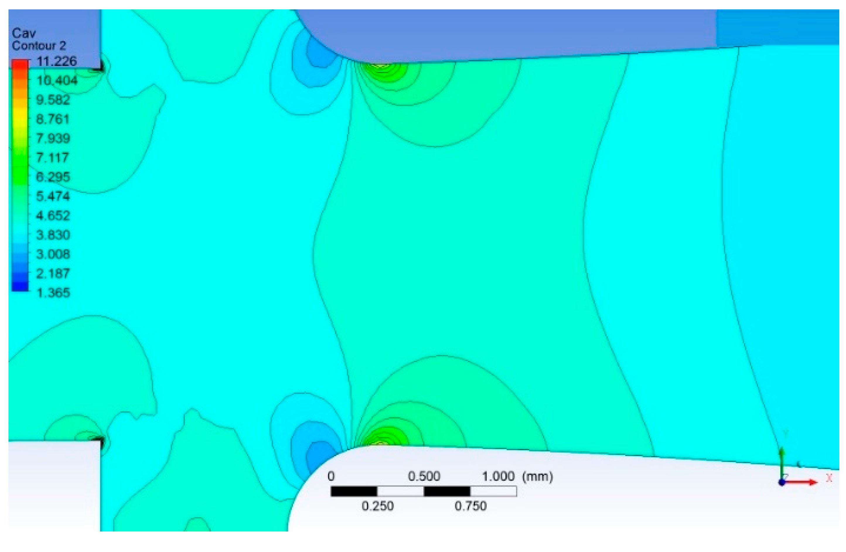
As previously mentioned, the risk of cavitation it is an issue for the fluid dynamics inside the device during operation. The following Cavitation-Risk Coefficient has been introduced:

$$C_{RC}=\left(p_{vap}/p\right)\times 100$$

(45)

The contours of the above function are plotted in order to check for zones of cavitation risk inside the model. If the local pressure is equal or higher than the vapor pressure, then the coefficient goes from 100% to lower values. In practice values around $C_{RC}=100\%$ are expected where there is incipient cavitation; $C_{RC}>100\%$ in regions where cavitation started and $C_{RC}<100\%$ for regions where cavitation is avoided. Figure 16 and Figure 17 report the contour lines for the above coefficient in case of inlet pressure equal to 1.0 (bar) and baseline geometry. For the reference configuration under study, the major risk is located in the Core Region of the ABD at the nozzle outlet section. This is due to the high fluid velocity reached in this section. Nevertheless, as the color scale reports, for this flow condition the risk is under the 12%, which is considered highly acceptable. After a simulation campaign by varying the inlet pressure, even a value of 2.5 (bar) and a maximum velocity of 30 m/s, the cavitation coefficient is below 85%. The risk of cavitation for the ABD configuration is therefore very low in a large range of operating conditions.

5. CFD Unsteady Analysis: The Switching Transient Phase

The Switching Transient Phase (STP) is the transitional phase, during the working regime of the ABD, when the main flow detaches from one curved wall and reattaches to the opposite wall, due to the effect of a pressure perturbation through the actuation port. This phase starts at time τ₀ when the perturbation takes place, and ends at the time τ_final, the instant when the flow is completely reattached and deviated. The operational time interval for the STP is therefore $\Delta {\tau }_{STP}={\tau }_{final}-{\tau }_0$.

It is very difficult to develop a mathematical model for the above time interval due to the complex flow physics associated to flow unsteadiness and turbulence. According to the available literature, with particular reference to the experimental characterization conducted by Tesaret al. [13], the STP time interval is related to:

• jet velocity at the nozzle section Uh;
• discharge channel deviation angle;
• actuation pressure;
• dynamic viscosity.

In case of configurations and devices similar to the present case and working with gases, the time interval is of the order of ${10}^{-3}$ s [14]. In case of water a value of the order of ${10}^{-2}$ s is expected because, even if the velocity of propagation of perturbations is higher due to the incompressibility of water, its density is thousand times higher than a gas like air, so the higher inertia of the fluid stream has a greater influence on the switching time interval. The above reference time has been used to set the time-step of the unsteady CFD analysis accordingly. 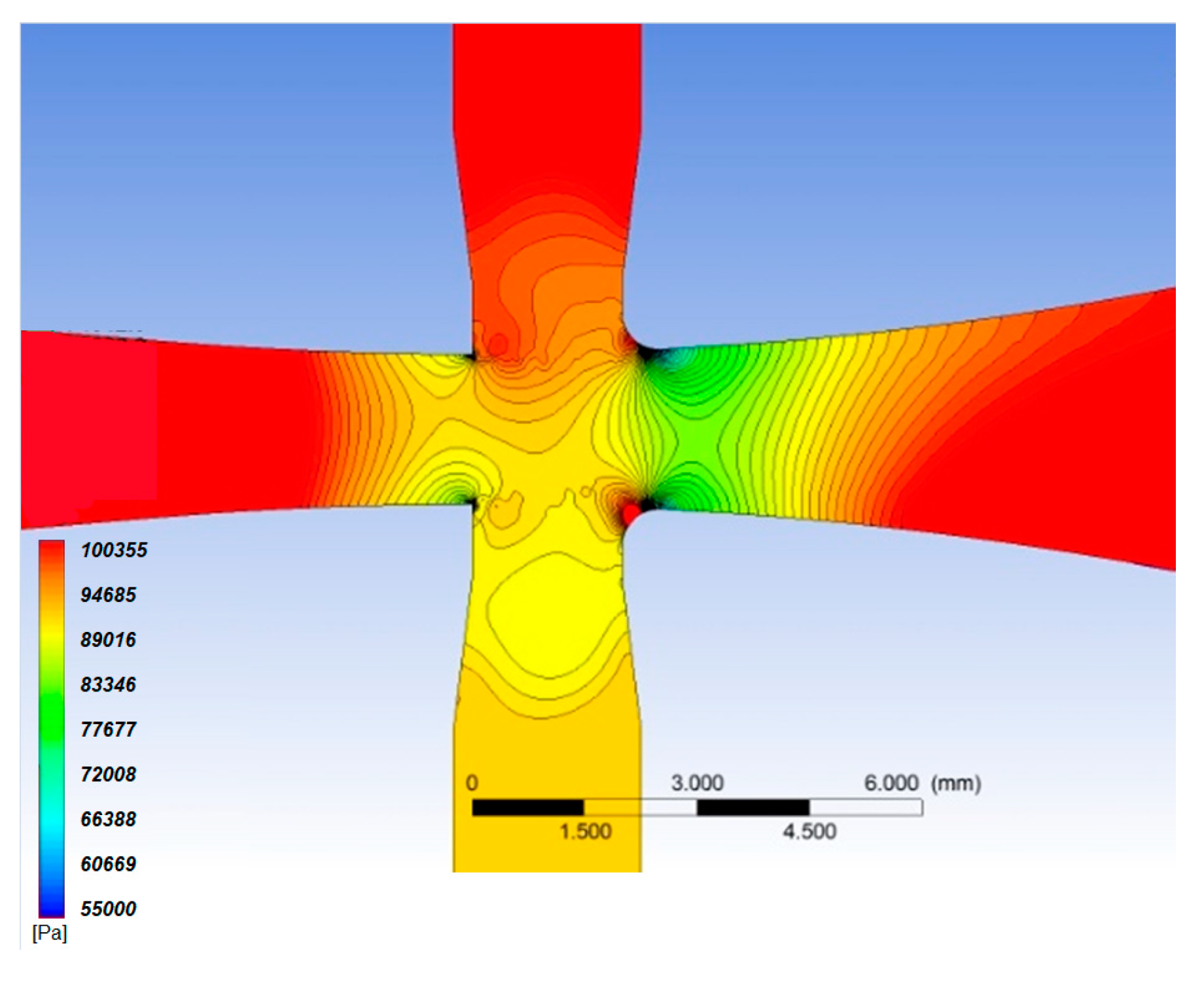In Figure 18 and Figure 19 the pressure contours at the instant immediately before τ₀ and at the time τ₀ (high pressure in the activation channel) are respectively shown. The symmetrical pressure distribution of Figure 18 is dramatically, instantaneously, changed at the time τ₀ corresponding to the opening of the upper actuation channel (Figure 19).

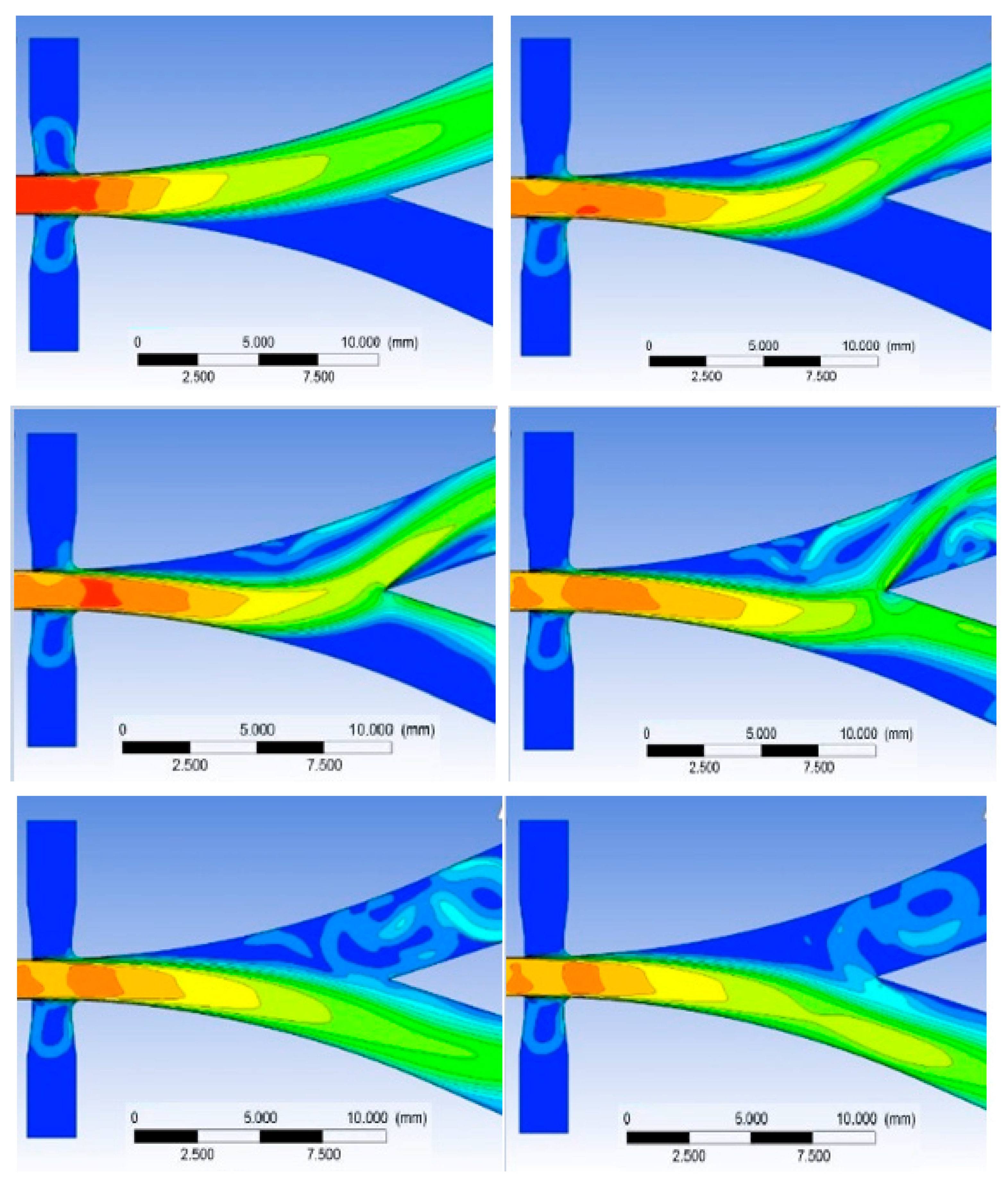
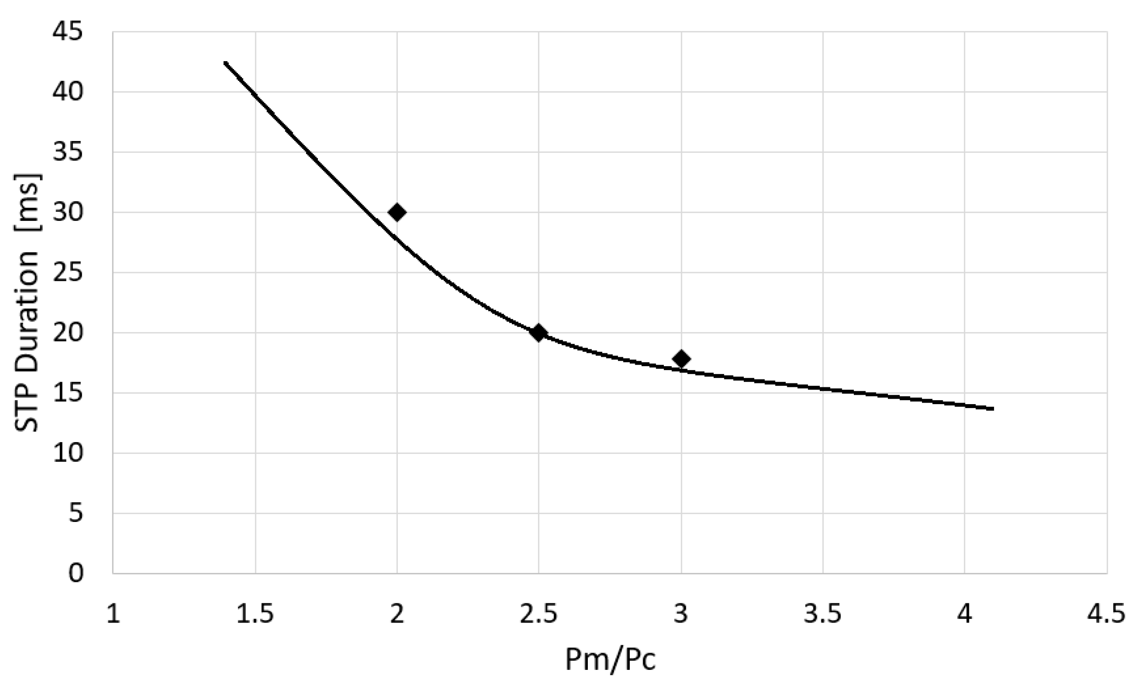
Because the pressure in the core region is much lower than the outlet pressure (Venturi effect), when the actuation ports opens, the suction effect drives the ABD to auto induce an actuation as soon as one of the side ports is opened. In Figure 20, the flow sequence during the STP is shown with the velocity contours and reported with a time interval of 5 × ${10}^{-3}$ s. After a simulation campaign with different operating conditions, it has been observed that, with a given pressure at the actuation port, the STP time interval is directly influenced by the maximum flow speed reached at the nozzle section. Figure 21 reports the $\Delta {\tau }_{STP}$ value with respect to the ratio between inlet pressure Pm and actuation pressure Pc.

The above curve can be used to predict the STP time with a prescribed pressure ratio or to find the actuation pressure, for a given inlet operating pressure, to get a prescribed time interval.

6. Experimental Tests

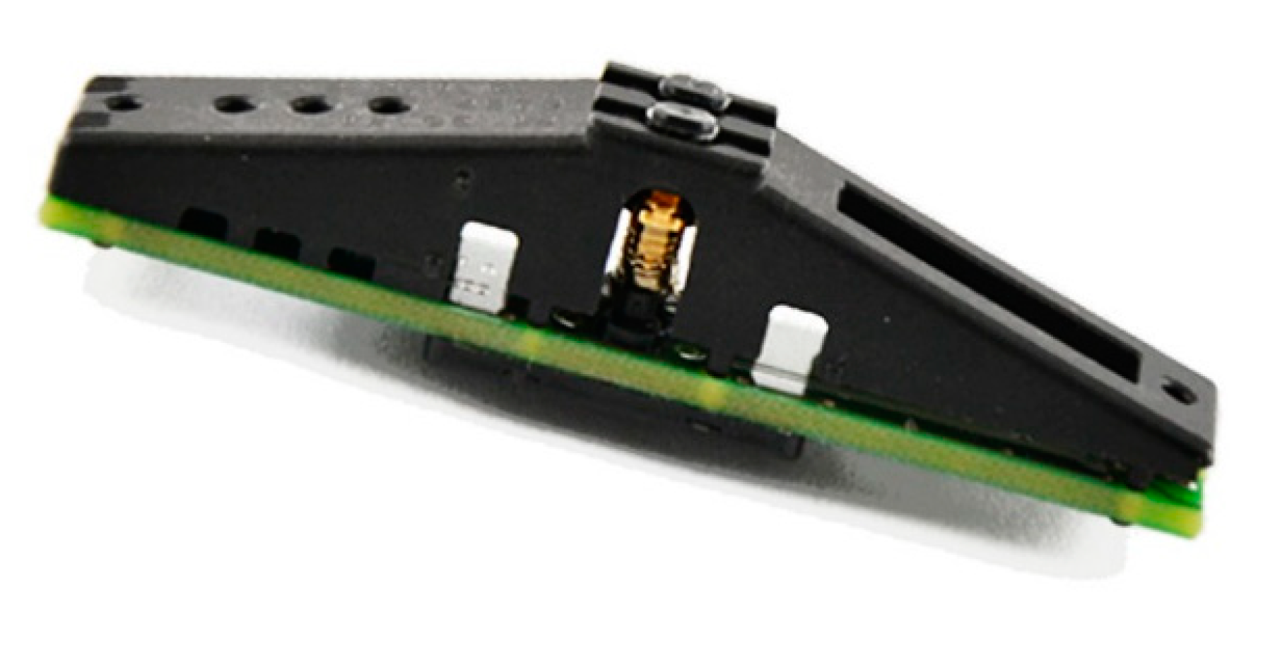
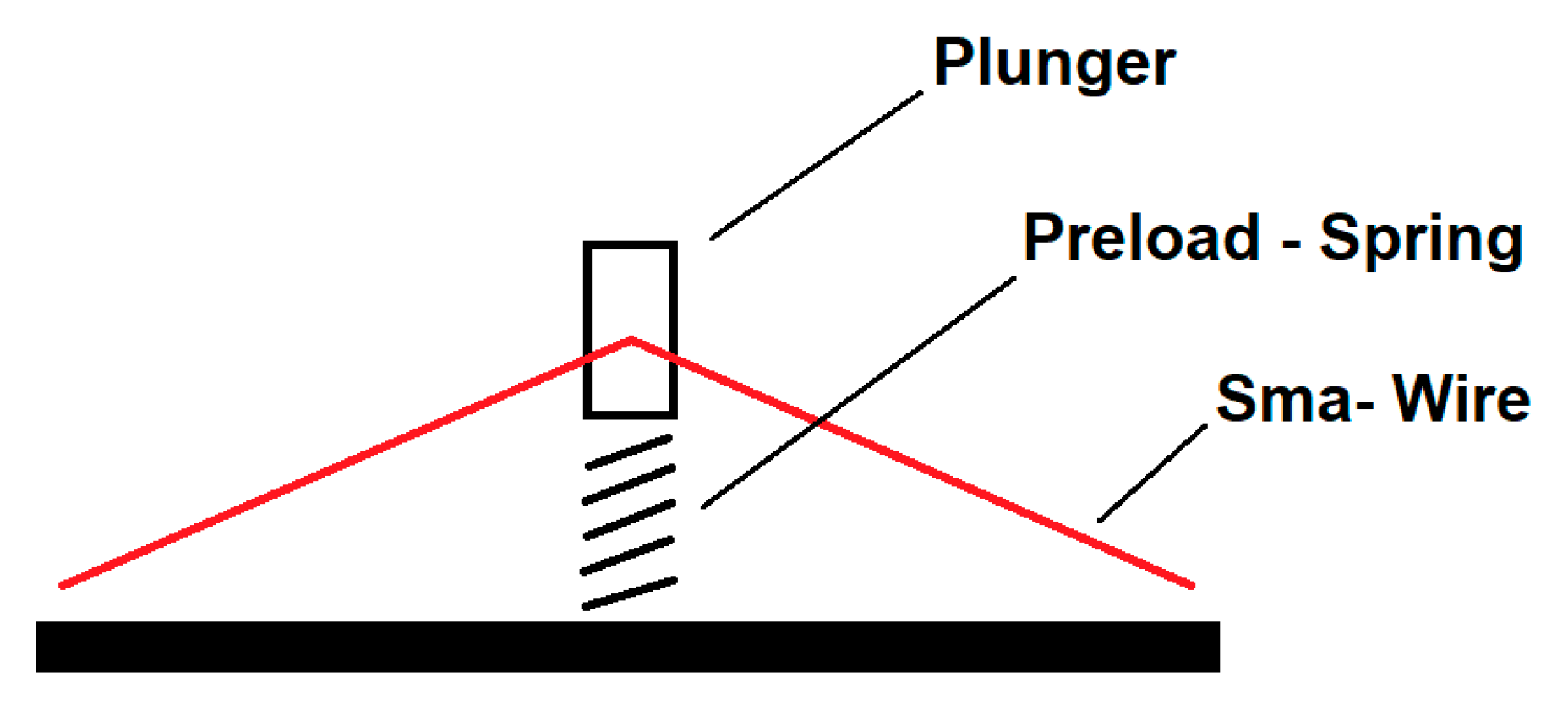
An experimental setup has been developed to check the operation of the fluidic device under different activation signals, as clearly reported by Comes [27]. A smart actuator to control the ABD actuation ports has been used. This device, developed for the automotive market by the Swiss company SAES-Getters, is shown in Figure 22. It consists of two independent plungers, each moved by a wire made of a special alloy of Nichel and Titanium, called Nitonol. Nitinol, also known as SMA (Shape Memory Alloy), is a very peculiar smart material able to gain super-elastic properties thanks to a solid-state transformation due to a moderate temperature change (about 70 °C). The SMA wire is installed to form an arc with its vertex fixed to the plunger (Figure 23). The SMA wire reaches a Martensitic state if heated using electric current and contracts; the arc therefore generates a force able to move the spring, necessary to keep in tension the wire and to pull the plunger down. In the following cooling phase (electric current switched off) the Nitinol wire recovers to the Austenitic phase (with a moderate hysteresis) to the initial length; the plunger goes back controlled by the spring. The Smart Actuator is equipped with rubber-made plungers to have adequate sealing performance. The SMA wires inside the actuator are 75 µm thick; the total amount of electric current is less than 0.7 A. The actuation phase is completed in 0.5 s while the cooling time is about 20% slower. 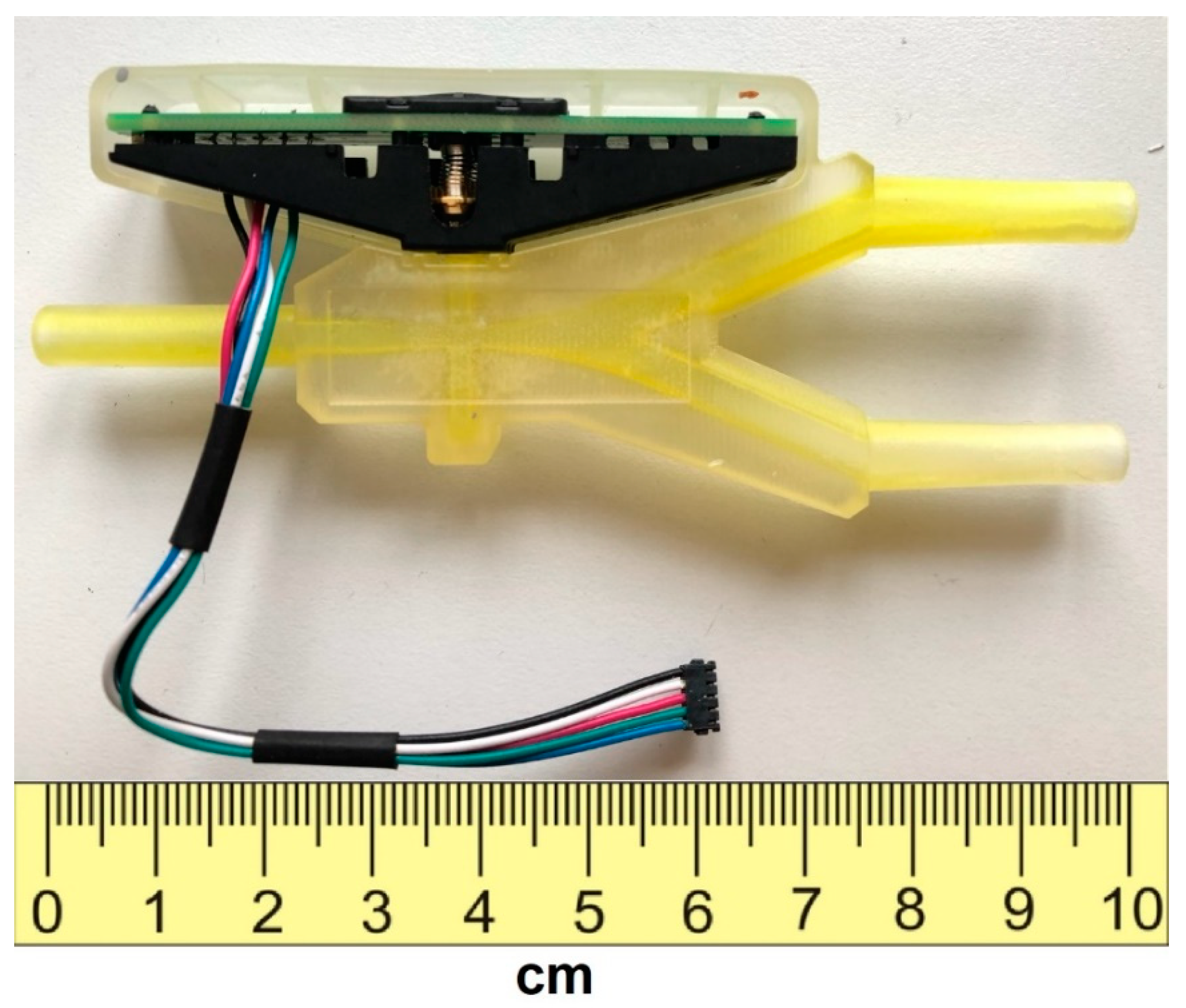Figure 24 shows the ABD prototype, built from additive manufacturing using Polyamide (3D printing), with the Smart Actuator integrated into the casing.

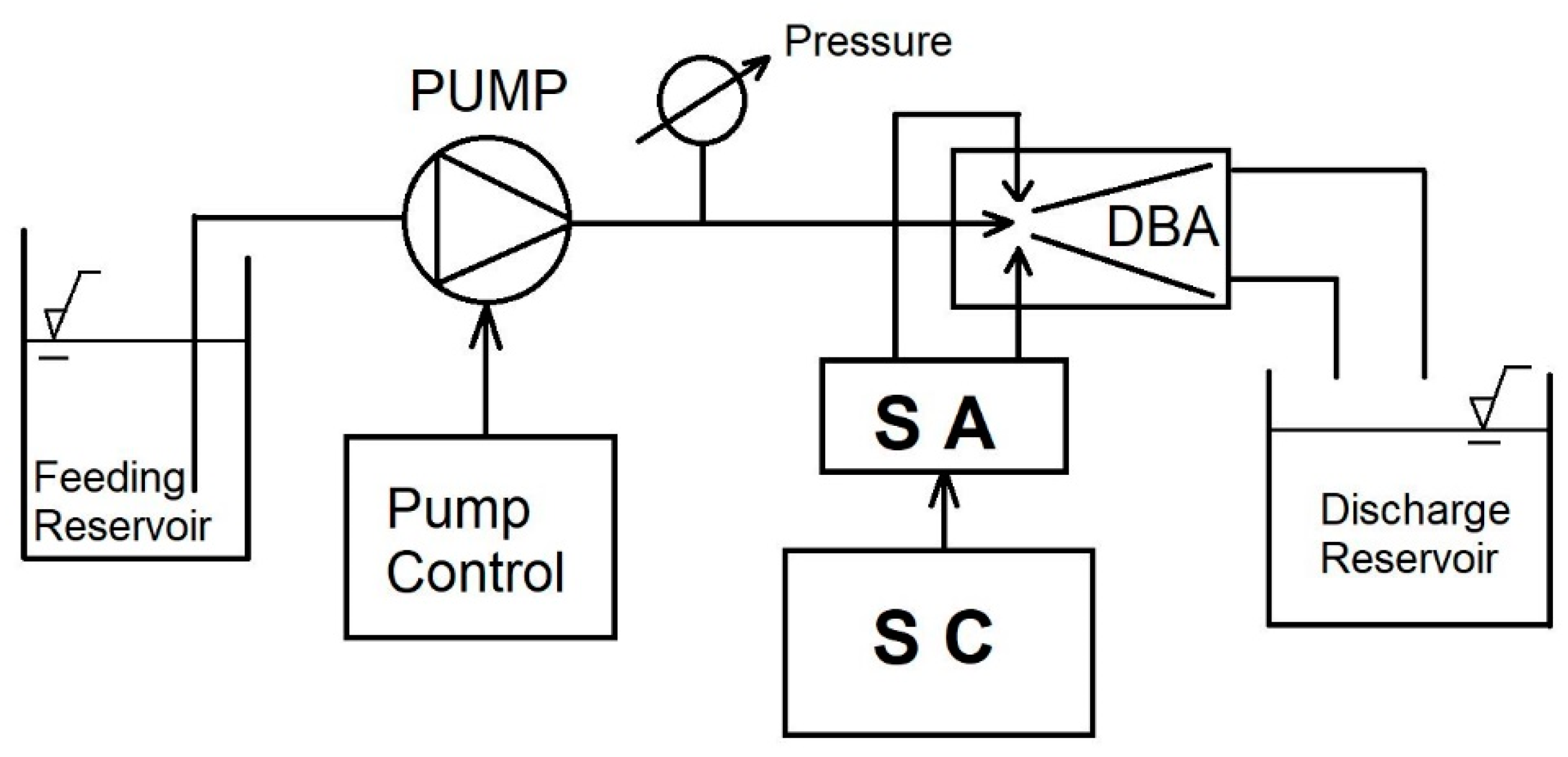
Two hydraulic test circuits have been conceived as shown Figure 25 and Figure 26. A smart actuator (SA) and a pushbutton (SC) control the switching process. In the first setup a gear pump is used to provide the working massflow to the ABD in the range 10–30 (lph), controlled by the pump motor. The pump pressure, in the range 1–2.5 (bar), is controlled using a pressure sensor (PS). 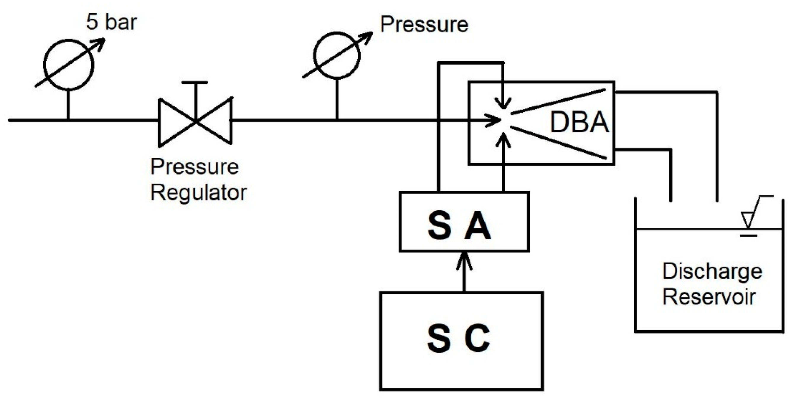The actuator has two plungers with movements electronically controlled: the ABD actuation ports are opened or closed (UP or DOWN in Figure 25). The volumetric flow rate is directly fixed by the rotational speed of the pump unit with a check on the inlet pressure. An alternative configuration circuit is shown in Figure 26. In this circuit a pressure regulator (PR), without mass flow rate control, guarantees the inlet pressure. The above circuits have been conceived because the fluidic device has a different response to fixed inlet flow rate or fixed inlet pressure. It is interesting to investigate the influence of the inlet pressure fluctuations (induced by the pump but not present with the reservoir supply) on the device response. With the circuit in Figure 26 a volumetric flow rate of over 300 (lph) has been obtained, moreover this configuration closely replicates the inlet condition used for the CFD simulations. The apparatus has been tested in the range 1-3 (bar) for inlet pressure (circuit Figure 26) and in the range 10–300 (lph) for inlet volumetric flowrate (circuit Figure 25).

The fluidic device has been extensively tested using the above circuits and tested under fixed inlet flow rate or inlet pressure. The following conclusions and considerations can be drawn. The test campaign with controlled inlet volumetric flow rate has highlighted the following positive issues for the device operation:

• the switching phase is started by simply opening the actuation ports with ambient pressure
• the switching phase is very fast (the order of 3 × 10⁻² s) and clean. The passive channel remains dry with suction of external air;
• the jet adhesion to the wall (Coanda effect) is strong and evident even with low flow rates.
• The following drawbacks have been observed:
• the device response is very sensitive to inlet flow fluctuations
• only low back pressure values (the order of 5% of the inlet pressure) are accepted for proper jet diversion.

When the fluidic device is operated with fixed inlet pressure, the following advantages are observed:

• higher resistance to back pressure;
• low sensitivity to inlet flow perturbations or fluctuations;
• instantaneous starting from dry conditions (device empty—only air).

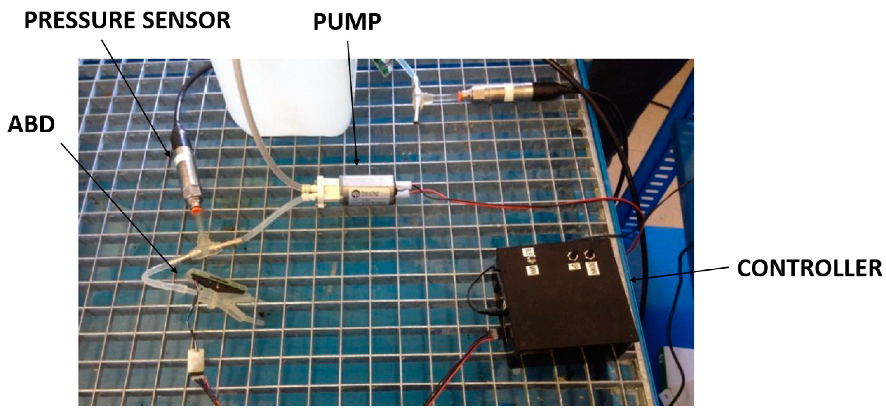
The main disadvantage of the device operation with given inlet pressure is the risk of cavitation. In Figure 27 a picture of the testing circuit (Figure 25) is shown. The ABD, with the actuator integrated in its own casing, results in a very compact device, with size comparable to the pressure transducer. The controller for the actuator consists of a switching panel used to separately control the ABD auxiliary ports. A gear pump is installed.

The test campaign has been useful to highlight the main advantages and drawbacks of the device with different operating strategies. Further tests are planned with the addition of instrumentation for the quantitative monitoring of the system performance with several operating cycles of different modes.

7. Conclusions

The mathematical model developed for the ABD device has been used to design one configuration that has been extensively investigated using CFD and tested in a preliminary experimental campaign. The main targets have been achieved. The theoretical model has been validated using CFD that has also allowed the setup of correlations for design parameters that need to be tuned in the design model. An interesting expertise has been developed for the design of bi-stable fluidic diverters that can be used to develop series of devices with the same operating principle. A relevant performance of these kind of devices is that a significant amount of flow energy can be controlled using a very low amount of energy in the input actuator having a stable and well-defined diverted jet as a result.