Qualitative Effects of Hydraulic Conductivity Distribution on Groundwater Flow in Heterogeneous Soils

Abstract

One of the most significant difficulties in subsurface hydrology is the considerable uncertainty in hydraulic conductivity values in the medium. This stimulates qualitative analysis of the effect of conductivity distribution on the solutions or on some components of the solutions of groundwater flow equations. This work is an attempt to develop a rigorous basis for deciding whether the solutions are monotonous with respect to hydraulic conductivity. Such monotonicity is analogous to the well-known comparison principles with respect to variations of initial data or external supplies. Some example problems are given in this paper, including a problem with a free boundary, in which the monotonous dependence of the solution on the conductivity distribution is proved rigorously. Examples are also given, in which monotonicity assumptions, despite being apparently obvious, are proved to be invalid.

1. Introduction

The use of mathematical models to solve practical problems of subsurface hydrology implies specifying many model parameters. These include the hydraulic properties of soils, the initial data, and the external inflow rates. Such characteristics show a high variability over spatial coordinates. This is especially true for the hydraulic conductivity, as its values can vary by several times or even orders of magnitude within the model domain even in geologically homogeneous media. When these source data cannot be determined with sufficient detail, the researcher, in what regards the majority of inputs, can rely only on data on the likely ranges of their variations. The result is that, as a general matter, a considerable portion of input data in engineering groundwater flow problems can be specified by guess with a high degree of arbitrariness. The chance to guess the correct values of parameters is clearly not high in this case, and the solutions of the problems based on such data will, most likely, be far from those required.

In this context, when solving practical engineering problems, one has to have an idea about the magnitude and the sign of the difference between the model solution with assumed input data and the solution that one would have with true, but unknown, parameter values. Such question will always arise in model calibration or when one tries to evaluate the accuracy and reliability of model calculations. In numerical studies, such problems are commonly solved with the use of sensitivity analysis. This rapidly developing field incorporates the ideas of small-perturbation theory, stochastic analysis, and many other methods. The analysis of the state of the art in this field falls beyond the focus of this study; therefore, we refer the reader to a recent review [1] and research articles [2,3]. It is worth noting that, if the number of unknown variables and the ranges of their possible variations are great, a thorough sensitivity analysis might require exceeding computational resources. This fact can be of importance for engineers dealing with applications if the objective of their work is not to prepare a scientific paper, but to perform a professional task. At the same time, the researchers can avoid such problem in some cases by assuming the characteristics of solutions of flow equations to be monotone functions of model parameters. For example, it is obvious that the position of groundwater table in an unconfined aquifer monotonously depends on the rate of external water inflow, i.e., the greater the inflow, the higher the level. Therefore, in the problems where groundwater table position is to be found and the external inflow rates are input data known with a considerable uncertainty, the rates of external inflow can be assigned maximal possible values (with a margin), thus making the calculated position of groundwater table a reliable upper estimate for the true value. Thus, the monotonicity allows this estimate to be obtained by a single calculation, avoiding the examination of many possible inflow rate values. This idea works well whatever the dimension of the parameter space, including the infinite-dimensional case for continuous-domain problems.

This assumption regarding the monotonous dependence of groundwater table position on external inflow in groundwater flow models is both intuitively obvious and mathematically rigorous. Textbooks on partial differential equations commonly contain such statements in the section devoted to the maximum and comparison principles (see, e.g., [4,5]). The monotonicity of solutions of non-stationary flow problems with respect to initial conditions has also been well studied ([6]); in particular, the rise of the initial groundwater level is followed by its rise in later time moments, other conditions being the same. This allows us to state that the solutions of flow problems with initial data chosen appropriately, i.e., with a margin, can be used as upper or lower estimates for solutions to the same problems with actual distributions of the initial data. Note that the methods used to prove the comparison theorems involve neither numerical approximations of models, nor conventional approaches to sensitivity analysis.

The monotonicity of the dependence of groundwater flow problem solutions on the distribution of the hydraulic conductivity has not been studied by mathematicians. At the same time, the engineering approaches to groundwater flow simulation often involve estimates based on the assumptions that some characteristics of the flow monotonically depend on the values of hydraulic conductivity. In the absence of rigorous mathematical proofs, such assumptions are based on the researcher’s intuition and regarded as obvious. This study gives examples of problems in which such assumptions can be proved rigorously, and, most importantly, counterexamples, in which seemingly obvious monotonicity hypotheses are proved to be erroneous. This is the goal of the paper. The examples and counterexamples presented here are continuous rather than numerical models. The monotonicity is proved with the use of variation methods similar to those commonly used to prove the comparison theorems [5,6].

A key factor in the construction of these counterexamples is the heterogeneity of the medium, as in the case of homogeneous media, the dependence of flow problem solutions on parameters commonly does not contradict intuition and can be easily substantiated. The issues of the qualitative properties of solutions considered in this article are not intended to be a consistent presentation of a complete mathematical theory; they are rather to be considered as an attempt to attract attention to the formulated problem. At the same time, the researchers who are focused on solving practical problems can find this article useful as a caution to be careful with conclusions based on the results of mathematical modeling of groundwater flow processes.

2. Problem Formulation and Results

2.1. The Problem of Water Inflow into an Open Water Body (a Pit)

To vividly demonstrate the problem described in the Introduction, we start with a detailed analysis of a simple example. We consider a stationary two-dimensional problem describing groundwater discharge from a confined aquifer into an open water body. Let the aquifer planar view be a ring-shaped domain $\mathrm{\Omega }$ in a plane with coordinates $x_1$, $x_2$ (Figure 1). In the hydraulic approximation (see, e.g., [7] Chap. X, [8] Chap. 8), the pressure head $u=u(x_1,x_2)$ in the aquifer depends only on the horizontal coordinates and satisfies the equations

$$\nabla ·q=0,q=-T\nabla u$$

(1)

where $\nabla =(\partial /\partial x_1,\partial /x_2)$ is the gradient operator, $q=(q_1,q_2)$ is water flow vector field, and $T=T(x_1,x_2)$ is the transmissivity. The latter parameter is determined by aquifer thickness and the distribution of hydraulic conductivity in it; therefore, it can vary over spatial coordinates. We assume that the inner contour of the ring $C_{int}$ is a boundary of an open water body with a fixed head $u=0$, and the head along the external boundary $C_{ext}$ is known and specified as a function $u=U\left(s\right)>0$, where s is the length along this curve. With the specified boundary conditions, the system of Equation (1) has a unique solution, provided that the distribution of transmissivity $T(x_1,x_2)$ is known.

Given the water flow distribution along boundaries, the total inflow into the water body can be calculated as

$$Q={\int }_{C_{int}}q·nds=-{\int }_{C_{ext}}q·nds$$

where n is the outward normal vector to the boundary of the flow domain $\mathrm{\Omega }$.

If the size of the aquifer is large and its hydraulic conductivity distribution is heterogeneous, the data on the distribution of transmissivity T all over the domain $\mathrm{\Omega }$ are difficult to collect. Generally, a few exploration wells are available to obtain reliable data on the geological structure of the aquifer, but these data can only be used to determine the possible ranges of transmissivity values in different parts of the aquifer. As the solution of Equation (1) cannot be found when parameter $T(x_1,x_2)$ is unknown, a natural step is to try to determine at least the ranges of possible values of the solution, for example, the values of discharge Q, assuming that the limits of possible values of transmissivity $T(x_1,x_2)$ are specified.

The approach based on successively trying all possible distributions of $T(x_1,x_2)$ with solving Equation (1) to obtain estimates for discharge Q is unrealistic. However, if we assume that the discharge Q monotonically increases with increasing transmissivity $T(x_1,x_2)$, then we can avoid the need to try all possible functions $T(x_1,x_2)$. In this case, it will be enough to consider only two distributions with maximal and minimal possible values of T and, solving appropriate problems, to obtain upper and lower estimates for Q. The exact formulation of the relevancy of the above assumption is as follows. Let $T_0(x_1,x_2)$ and $T_1(x_1,x_2)$ be two different distributions of transmissivity with $T_0(x_1,x_2)\le T_1(x_1,x_2)$ all over the flow domain, and $Q^{\left(0\right)}$ and $Q^{\left(1\right)}$ be the corresponding values of the total discharge, calculated with the use of Equation (1). Can we expect that $Q^{\left(0\right)}\le Q^{\left(1\right)}$ in this case?

If we consider a homogeneous aquifer with a constant transmissivity T, then the total discharge Q is proportional to T, as follows from dimensional considerations. In that case, the monotonous dependence of Q on T is obvious and needs no substantiation. The assumption that the dependence is still monotonous in the case of variable coefficients looks so natural and agreeing with engineering intuition that even the question of whether this is always so can astonish some researchers. This makes even more surprising the following statement.

Proposition 1.

If the head at the inflow boundary of the aquifer is constant, i.e., $U\left(s\right)\equiv const>0$, then the dependence of Q on $T(x_1,x_2)$ is monotonous. However, if $U\left(s\right)\ne const$, then, for any transmissivity distribution $T_0(x_1,x_2)$, there exists a distribution $T_1(x_1,x_2)$, such that $T_1(x_1,x_2)\ge T_0(x_1,x_2)$ in all points of domain Ω, but $Q^{\left(1\right)}<Q^{\left(0\right)}$.

This mathematical result means that, in heterogeneous aquifers at $U\left(s\right)\ne const$, correct estimates of the total discharge cannot be constructed based on the monotonicity assumption. The proof of Proposition 1 is given in Section 3.1. Note that the results formulated here keep true in the case of anisotropic medium, when the transmissivity $T(x_1,x_2)$ in Equation (1) is a matrix-valued rather than a scalar function of coordinates. In the case of matrices, the relationship $T_1(x_1,x_2)\ge T_0(x_1,x_2)$ is assumed to mean that all eigenvalues of the difference $T_1-T_0$ are nonnegative.

2.2. The Rate of Groundwater Table Rise in the Process of Flooding from Contour Ditches

Let an unconfined aquifer be located between two parallel open canals and underlain by an impermeable bed. A vertical cross-section $ABCD$ of this aquifer is given in Figure 2. We consider a two-dimensional profile problem of groundwater flow caused by an abrupt and simultaneous level rise in the left and right canals. Suppose that water table in the soil before time $t=0$ lies at a height $h_0$ and coincides with the levels in the canals, while at $t=0+$ the level of both canals instantaneously rises to $H>h_0$ and remains constant for $t>0$. The state of groundwater at $t>0$ and, in particular, the dynamics of its free surface $y=h(t,x)$ are to be determined. In practice, this type of problems arises in land irrigation.

Boussinesq approximation (see, e.g., [7] Chap. X, [8] Chap. 8) is unacceptable for the problem, at least, at the first stage of the process. Therefore, a two-dimensional flow model should be used to describe water flow in the aquifer. In this case, the state of groundwater in the flow domain can be described by the distribution of water head $u=u(t,x,y)$ and flux vector $q=(q_x,q_y)$, satisfying the equations

$$\nabla ·q=0,q=-K\nabla u$$

(2)

where $\nabla =(\partial /\partial x,\partial /\partial y)$, and $K=K(x,y)$ is a symmetrical and positively defined matrix of hydraulic conductivity for inhomogeneous and anisotropic medium. The domain above the flow zone is assumed dry, i.e., the residual water content there is not greater than the threshold above which water motion becomes possible. If aquifer recharge is negligible, then the conditions at the free boundary, separating the dry and wet zones and coinciding with the plot of the function $y=h(t,x)$ to be determined, read

$$u(t,x,y)=h(t,x)\mathrm{and}{q}_y=m\frac{\partial h}{\partial t}+q_x\frac{\partial h}{\partial x}\mathrm{at}y=h(t,x),$$

(3)

where $m=m(x,y)$ is a specified distribution of effective porosity coefficient. The aquifer bed is assumed horizontal and impermeable, i.e., $q_y(t,x,y)=0$ at $y=0$. At the boundaries of the flow zone with the left and right open canals, we specify constant head values at $t>0$:

$$u(t,x,y)=H\mathrm{on}AD\mathrm{and} \mathrm{on}BC\mathrm{at}y<H.$$

(4)

Problem formulation is completed by the initial condition $h(0,x)=h_0$.

The relationships in Equations (2)–(4) correspond to the so-called strong formulation of the problem of groundwater flow with a free surface. In this formulation, the existence of a solution is not guaranteed. A solution existence theorem is given in [9], limited to a rectangular cross-section and homogeneous medium. As shown by examples in previous studies [10,11], the solution may not exist in the case of homogeneous medium. To ensure the solvability, the problem in Equations (2)–(4) can be presented in another form, which the authors of [12,13] called weak. The solvability in weak sense of a stationary problem for a dam and other similar free-boundary problems is discussed in detail in [10,14]. In the weak formulation, the solution is described by another set of functions, and the study of the dependence of these solutions on hydraulic conductivity distribution becomes much more complicated. Therefore, here, we limit our analysis to a strong formulation of the problem, assuming its solution to exist.

If $K(x,y)=kI$ and $k=const>0$, i.e., the medium is homogeneous and isotropic, dimensional analysis shows that the unknown groundwater table $h=h(t,x)$ in the problem under consideration depends monotonically on the constant hydraulic conductivity k. This could suggest an assumption that this monotonicity holds for heterogeneous medium as well, i.e., the greater the hydraulic conductivity in a medium, the faster the recovery of groundwater table during inundation. An exact formulation of this hypothesis is as follows: if $K_0(x,y)$ and $K_1(x,y)$ are two different distributions of the hydraulic conductivity tensor in the medium such that $K_0(x,y)\le K_1(x,y)$ everywhere, and $h^{\left(0\right)}(t,x)$ and $h^{\left(1\right)}(t,x)$ are the corresponding solutions of the problem in Equations (2)–(4), then the inequality $h^{\left(0\right)}(t,x)\le h^{\left(1\right)}(t,x)$ will hold for any t and x. The main result of this section is the proof that this natural assumption is not quite correct. For this purpose, we give a counterexample in which the inequality $h^{\left(0\right)}(t,x)\le h^{\left(1\right)}(t,x)$ will be true not for all but for large enough values of time t, while at the initial stages of the process, we have $h^{\left(0\right)}(t,x)>h^{\left(1\right)}(t,x)$.

To construct the counterexample, we use a two-layer aquifer system given in Figure 3. The domain $ABCD$ is a rectangle, the bottom and top parts of which are beds with hydraulic conductivities $k_{+}$ and $k_{-}$, respectively, with $k_{+}>k_{-}$. The distribution of the corresponding isotropic hydraulic conductivity tensor has the form: $K_0(x,y)=k_{+}I$ at $y<H_1$ and $K_0(x,y)=k_{-}I$ at $y>H_1$, where $H_1$ is the thickness of the bottom bed. The second medium will be a homogenous structure with a hydraulic conductivity tensor $K_1(x,y)\equiv k_{+}I$. Now, in any point of the rectangle $ABCD$, we have $K_0(x,y)\le K_1(x,y)$. Figure 4 shows numerical plots of the levels $h^{\left(0\right)}(t,x)$ and $h^{\left(1\right)}(t,x)$ as functions of time in the central point $x=L/2$ between the canals. This result shows that $h^{\left(0\right)}(t,x)>h^{\left(1\right)}(t,x)$ at the initial stage of the process. This refutes the assumption of monotonicity of the water table level with respect to hydraulic conductivity. The calculations were made with the following parameter values: $L=108$ m, $H=8.4$ m, $h_0=5$ m, $H_1=4.5$ m, $k_{+}=1$ m/day, $k_{-}=0.01$ m/day, and $m=0.2$.

The effect of faster level rise in the case of an overlying low-permeability bed, as shown in Figure 4, is highly sensitive to parameter values. This effect manifests itself when the parameters satisfy the conditions $h_0>H_1$, $H<<L$, $k_{-}<<k_{+}$, and $k_{-}/k_{+}\sim {(H/L)}^2$. The physical mechanisms underlying this effect are as follows.

When the difference between the hydraulic conductivities $k_{-}$ and $k_{+}$ is not very large, for example, when ${(H/L)}^2<<k_{-}/k_{+}<1$, the process under consideration can be described with Dupuit–Boussinesq approximation. In this case, the head in the flow zone is assumed constant over the vertical, i.e., $u(t,x,y)\equiv h(t,x)$. It can be shown that, with such one-dimensional approximation, the level rise in the two-layer structure will not be faster than that in the homogenous one. However, if ${(H/L)}^2\sim k_{-}/k_{+}<<1$, Dupuit–Boussinesq approximation is inapplicable because, in this case, the head becomes constant along the vertical only in the more permeable bottom layer, rather than all over the vertical. Engineering applications in such situations commonly rely on another one-dimensional approximation based on Girinskii–Myatiev hypothesis [15,16]. In particular, Manukyan [17] developed this approach for problems of peatland rewetting for areas with appropriate geological structure of the medium. In the Girinskii–Myatiev approximation, it is assumed that the head in the low-permeability layer can be approximated by a linear function of coordinate y. Now, to describe the flow, two sought variables are needed, namely, the groundwater table in the top layer $h=h(t,x)$ and the head in the bottom layer $u=u(t,x)$. They can be found from the following one-dimensional equations

$$k_{+}H\frac{{\partial }^{2}u}{\partial x^2}+k_{-}\frac{h-u}{h-H_1}=0,m\frac{\partial h}{\partial t}+k_{-}\frac{h-u}{h-H_1}=0$$

(5)

with the boundary and initial conditions

$$u(t,0)=u(t,L)=H,h(0,x)=h_0.$$

With these conditions substituted into Equation (5) at $t=0$, one can explicitly calculate the rate of level rise at the initial moment $\partial h(0,x)/\partial t$, which is strictly positive over the interval $0<x<L$. An analogous calculation of the same value for a homogeneous structure with the use of the original Equations (2)–(4) or their simplified Dupuit–Boussinesq version leads to the equality $\partial h(0,x)/\partial t\equiv 0$. Therefore, at the initial stage of the process, the values of $h^{\left(0\right)}(t,x)$ in the two-layer aquifer lie above the level $h^{\left(1\right)}(t,x)$ in the homogeneous medium. In the case of a higher contrast between the permeability of the top and bottom layers, i.e., at $k_{-}/k_{+}<<{(H/L)}^2$, the rate of head rise in the bottom layer increases (at $k_{-}=0$, the value of $u(t,x)$ will instantaneously attain at $t=0+$ its maximal possible value $u=H$), while the increase rate of the level $h(t,x)$, in virtue of Equation (5), conversely, drops, to become zero at $k_{-}=0$. Therefore, the time interval within which the plot $h^{\left(0\right)}(t,L/2)$ lies above the plot $h^{\left(1\right)}(t,L/2)$ in Figure 4 decreases and the effect of faster level rise becomes insignificant.

At greater values of time t, in the particular case considered above, the plot of function $y=h^{\left(1\right)}(t,L/2)$ in Figure 4 lies higher than the plot of $y=h^{\left(0\right)}(t,L/2)$. This property holds in the general situation with an arbitrary distribution of hydraulic conductivity in the flow domain $ABCD$. The exact formulation of this statement is the following.

Proposition 2.

As soon as $K_0(x,y)<K_1(x,y)$ everywhere in the flow domain $ABCD$, the inequality $h^{\left(1\right)}(t,x)>h^{\left(0\right)}(t,x)$ will hold for the solutions to the problem in Equations (2)–(4) at sufficiently large values of time t.

Therefore, the dependence of the rate of groundwater table rise on hydraulic conductivity during inundation becomes monotonous only after a long enough time. In this, weaker, sense, the intuitively evident rule “the greater the conductivity, the faster water level stabilization” is correct. The proof of Proposition 2 is given in Section 3.2.

3. Mathematical Proofs

3.1. The Proof of Proposition 1

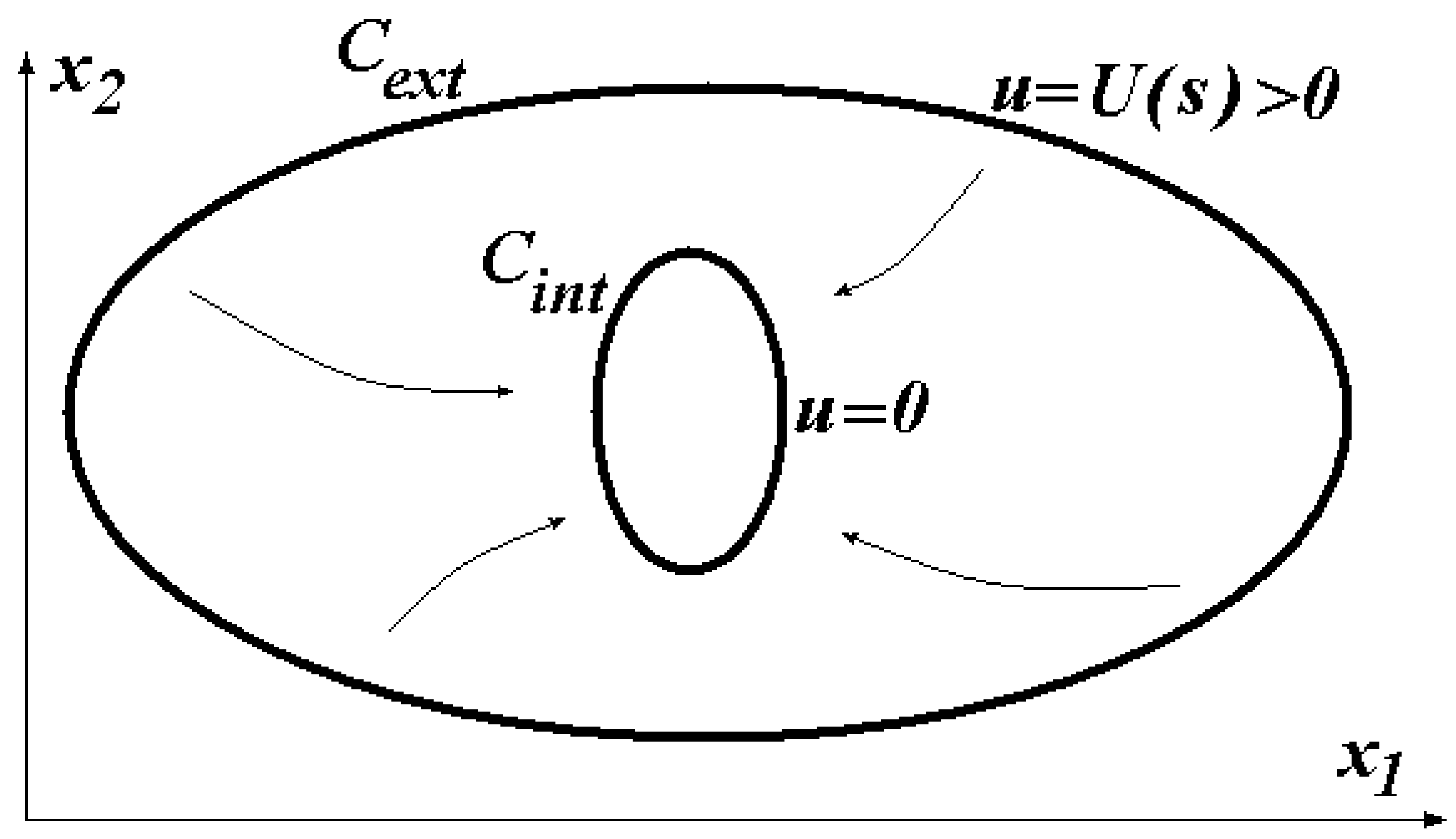
We give a brief proof of the statements formulated in Section 2.1 regarding the discharge from a confined aquifer into an open water body. We consider an anisotropic case with the distributions of transmissivity $T_0(x_1,x_2)$ and $T_1(x_1,x_2)$ assumed to be tensors, for which $T_0(x_1,x_2)\le T_1(x_1,x_2)$ everywhere in the domain $\mathrm{\Omega }$ shown in Figure 1. We denote the nonnegative difference between these tensors by $M(x_1,x_2)=T_1(x_1,x_2)-T_0(x_1,x_2)$. For an auxiliary parameter $\tau$, $0\le \tau \le 1$, we define a one-dimensional family of tensors $T_{\tau }(x_1,x_2)=T_0(x_1,x_2)+\tau M(x_1,x_2)$. At $\tau =0$ and $\tau =1$, the tensor $T_{\tau }(x_1,x_2)$ coincides with $T_0(x_1,x_2)$ and $T_1(x_1,x_2)$, respectively. The solution to the problem in Equation (1) with tensor $T_{\tau }(x_1,x_2)$ as a matrix of coefficients is denoted by $u=u^{\left(\tau \right)}(x_1,x_2)$ and the corresponding discharge value by $Q=Q^{\left(\tau \right)}$. Thus, the family of heads $u^{\left(\tau \right)}(x_1,x_2)$ satisfies the equations

$$q^{\left(\tau \right)}=-T_{\tau }(x_1,x_2)\nabla u^{\left(\tau \right)}(x_1,x_2),\nabla ·q^{\left(\tau \right)}=0\mathrm{in}\mathrm{\Omega },$$

(6)

$$u^{\left(\tau \right)}(x_1,x_2)=0\mathrm{on}{C}_{int},u^{\left(\tau \right)}(x_1,x_2)=U\left(s\right)\mathrm{on}{C}_{ext}.$$

(7)

Owing to the incompressibility condition, we have for the discharge value

$$Q^{\left(\tau \right)}={\int }_{C_{int}}{q}^{\left(\tau \right)}·nds=-{\int }_{C_{ext}}{q}^{\left(\tau \right)}·nds$$

(8)

where n is the outer normal to the boundary of domain $\mathrm{\Omega }$.

Let us consider a problem, analogous to Equations (6) and (7), with a unit Dirichlet condition on the outer contour $C_{ext}$ of domain $\mathrm{\Omega }$. Its solution $v^{\left(\tau \right)}(x_1,x_2)$ satisfies the equations

$$\nabla ·T_{\tau }(x_1,x_2)\nabla v^{\left(\tau \right)}(x_1,x_2)=0,$$

(9)

$$v^{\left(\tau \right)}(x_1,x_2)=0\mathrm{on}{C}_{int},v^{\left(\tau \right)}(x_1,x_2)=1\mathrm{on}{C}_{ext}.$$

(10)

Multiplying the second part of Equation (6) by $v^{\left(\tau \right)}(x_1,x_2)$ and integrating the product over the domain $\mathrm{\Omega }$ with Equations (8) and (10) taken into account, we obtain the following expression for the discharge:

$$\int {\int }_{\mathrm{\Omega }}{T}_{\tau }\nabla u^{\left(\tau \right)}·\nabla v^{\left(\tau \right)}d{x}_{1}d{x}_2=-{\int }_{C_{ext}}{q}^{\left(\tau \right)}·nds=Q^{\left(\tau \right)}.$$

(11)

Finally, the differentiation of this expression with respect to parameter $\tau$ yields the equality

$$\frac{d}{d\tau }{Q}^{\left(\tau \right)}=\int {\int }_{\mathrm{\Omega }}M\nabla u^{\left(\tau \right)}·\nabla v^{\left(\tau \right)}d{x}_{1}d{x}_2$$

(12)

because $d{T}_{\tau }/d\tau =M$, and the terms with derivatives of functions $u^{\left(\tau \right)}$ and $v^{\left(\tau \right)}$ with respect to $\tau$ under the double integral in the left part of Equation (11) vanish after integration by parts in virtue of Equations (6), (7), (9) and (10).

If $U\left(s\right)\equiv U_0=const>0$, then functions $u^{\left(\tau \right)}$ and $v^{\left(\tau \right)}$ are proportional and $\nabla u^{\left(\tau \right)}(x_1,x_2)=U_0\nabla v^{\left(\tau \right)}(x_1,x_2)$ in virtue of the linearity of the problems in Equations (6), (7), (9) and (10). Now, the equality in Equation (12) yields $d{Q}^{\left(\tau \right)}/d\tau \ge 0$, because the tensor $M(x_1,x_2)$ is nonnegative. Therefore, in this case, we have $Q^{\left(0\right)}\le Q^{\left(1\right)}$, i.e., the discharge is monotonic with respect to transmissivity coefficients.

If, conversely, $U\left(s\right)\ne const$, the solutions of the problems in Equations (6), (7), (9) and (10) are not proportional, whatever the value of $\tau$, and the gradients of those solutions, $\nabla u^{\left(\tau \right)}$ and $\nabla v^{\left(\tau \right)}$, are nonzero and nonparallel on a set of points $(x_1,x_2)$ with a nonzero measure. This holds true, at least for small neighborhoods of the segments of the outer contour $C_{ext}$ of domain $\mathrm{\Omega }$, where $dU/ds\ne 0$, because, in these segments, the vector $\nabla v^{\left(\tau \right)}$ is perpendicular to the boundary, while the vector $\nabla u^{\left(\tau \right)}$ is not. For a fixed value of $\tau$, for example, for $\tau =0$, in all such points a positively defined matrix $M(x_1,x_2)$ can be chosen, such that $M\nabla u^{\left(\tau \right)}·\nabla v^{\left(\tau \right)}<0$, while in other points we can set $M(x_1,x_2)=0$. Now, the inequality $d{Q}^{\left(\tau \right)}/d\tau <0$ at $\tau =0$ will follow from Equation (12). Therefore, at sufficiently small values of parameter $\tau$, the inequality $Q^{\left(0\right)}>Q^{\left(\tau \right)}$ will hold, while $T_0(x_1,x_2)\le T_{\tau }(x_1,x_2)$. This proves that the dependence of discharge Q on transmissivity coefficients is non-monotone in the general case.

If we limit ourselves to isotrophic distributions of transmissivity coefficients, i.e., assume the distributions $T_0(x_1,x_2)$, $T_1(x_1,x_2)$, and $M(x_1,x_2)$ to be scalar functions rather than tensors, then the above reasoning about the absence of monotonicity at $U\left(s\right)\ne const$ will require some supplement. Indeed, if the vectors $\nabla u^{\left(\tau \right)}$ and $\nabla v^{\left(\tau \right)}$, though not parallel, form an acute angle with one another everywhere in $\mathrm{\Omega }$, then it would be impossible to choose a nonnegative scalar function $M(x_1,x_2)$, such that the integral in Equation (12) be negative. This obstacle can be overcome by using the ideas of the homogenization theory of elliptic operators (see [18]).

The main result of this theory is that, if the distribution of coefficients $T(x_1,x_2)$ in Equation (1) has a fine structure with a small characteristic spatial scale (e.g., periodic in both variables with a period $\epsilon <<1$), then the solutions of boundary-value problems at $\epsilon \to 0$ will be close to the solutions of analogous problems with some effective distribution $T_{eff}$, not depending on $\epsilon$. In this case, the limiting distribution $T_{eff}$ can be anisotropic, even if the coefficients in the original problems at any fixed $\epsilon >0$ are isotropic. Based on this fact, the absence of monotonicity can be proved in two steps. In the first step, a nonnegative tensor distribution $M(x_1,x_2)$ is to be chosen such that the right-hand part of Equation (12) is negative at $\tau =0$. This distribution can be anisotropic; therefore, the transmissivity tensor $T_{\tau }(x_1,x_2)=T_0(x_1,x_2)+\tau M(x_1,x_2)$, for which the inequality $Q^{\left(0\right)}>Q^{\left(\tau \right)}$ holds for small values of $\tau$, may also be anisotropic.

In the second step, we fix the value of parameter $\tau >0$ for which $Q^{\left(0\right)}>Q^{\left(\tau \right)}$, and introduce a two-component composite medium consisting of two different isotropic media with transmissivities $T_0(x_1,x_2)$ and $T_0(x_1,x_2)+M^{\prime }(x_1,x_2)$ where $M^{\prime }(x_1,x_2)$ is a nonnegative scalar function to be found. To describe the distribution of both components within the aquifer, we consider a function $T(x_1,x_2,y_1,y_2)$ which is 1-periodic with respect to $y_1$ and $y_2$ and, for any fixed $x_1,x_2$, takes only two values, namely $T_0(x_1,x_2)$ and $T_0(x_1,x_2)+M^{\prime }(x_1,x_2)$. Let us take the transmissivity distribution of the above mentioned composite in the form $T^{\left(\epsilon \right)}(x_1,x_2)=T(x_1,x_2,x_1/\epsilon ,x_2/\epsilon )$ where $\epsilon >0$ is a small parameter. At any point $(x_1,x_2)$ of the aquifer, the arguments $x_1/\epsilon ,x_2/\epsilon$ are so-called fast variables. They are responsible for the micro-geometry of the composite in the $\epsilon$-neighbourhood of this point. The transmissivities of both components and the geometric parameters of their distribution within periodicity cells are not assumed uniform overall the flow domain. The first pair of arguments in the expression for the function $T(x_1,x_2,y_1,y_2)$ serves to describe slow variations of these macroscopic parameters within the aquifer. In approaches to the homogenization theory, such small-scaled composite structures are called locally periodic. In contrast with strictly periodic composites, the effective transmissivity tensor $T_{eff}(x_1,x_2)$ for them inherits the slow variations of macroscopic properties and depends on $x_1,x_2$. The value of the effective tensor is determined by the microstructure of the composite, i.e. by the particular form of the function $T(x_1,x_2,y_1,y_2)$, which is not specified yet.

Let us denote by $Q_{\epsilon }$ and $Q_{eff}$ the flow rates for the composite and effective aquifers, respectively. Then, in accordance with the homogenization theory, $Q_{\epsilon }$ converges to $Q_{eff}$ as $\epsilon \to 0$. If, occasionally, the distribution of effective transmissivity $T_{eff}(x_1,x_2)$ coincides with the distribution of $T_{\tau }(x_1,x_2)$, then $Q_{eff}=Q^{\left(\tau \right)}<Q^{\left(0\right)}$. In this case, the inequality $Q_{\epsilon }<Q^{\left(0\right)}$ will be valid for sufficiently small values of $\epsilon$. Since the composite medium is isotropic, it could be taken in place of the desired counterexample. Thus, it remans to construct a local geometry of the composite and find a nonnegative function $M^{\prime }(x_1,x_2)$ providing the prescribed values of the effective transmissivity $T_{eff}(x_1,x_2)=T_{\tau }(x_1,x_2)$ for any $x_1$ and $x_2$. This is a typical inverse problem of the homogenization theory. In the case of two-component composites, it is thoroughly studied. There are different ways to provide desirable designs of the composites. One of them is given in [19], and references for the others can be found there. Since the microstructure with the required properties is not unique, there is no reason to give here a precise description of a particular example of solution in explicit form. Right now, it is important that the microstructures with the required properties exist. This completes the proof of Proposition 1.

3.2. The Proof of Proposition 2

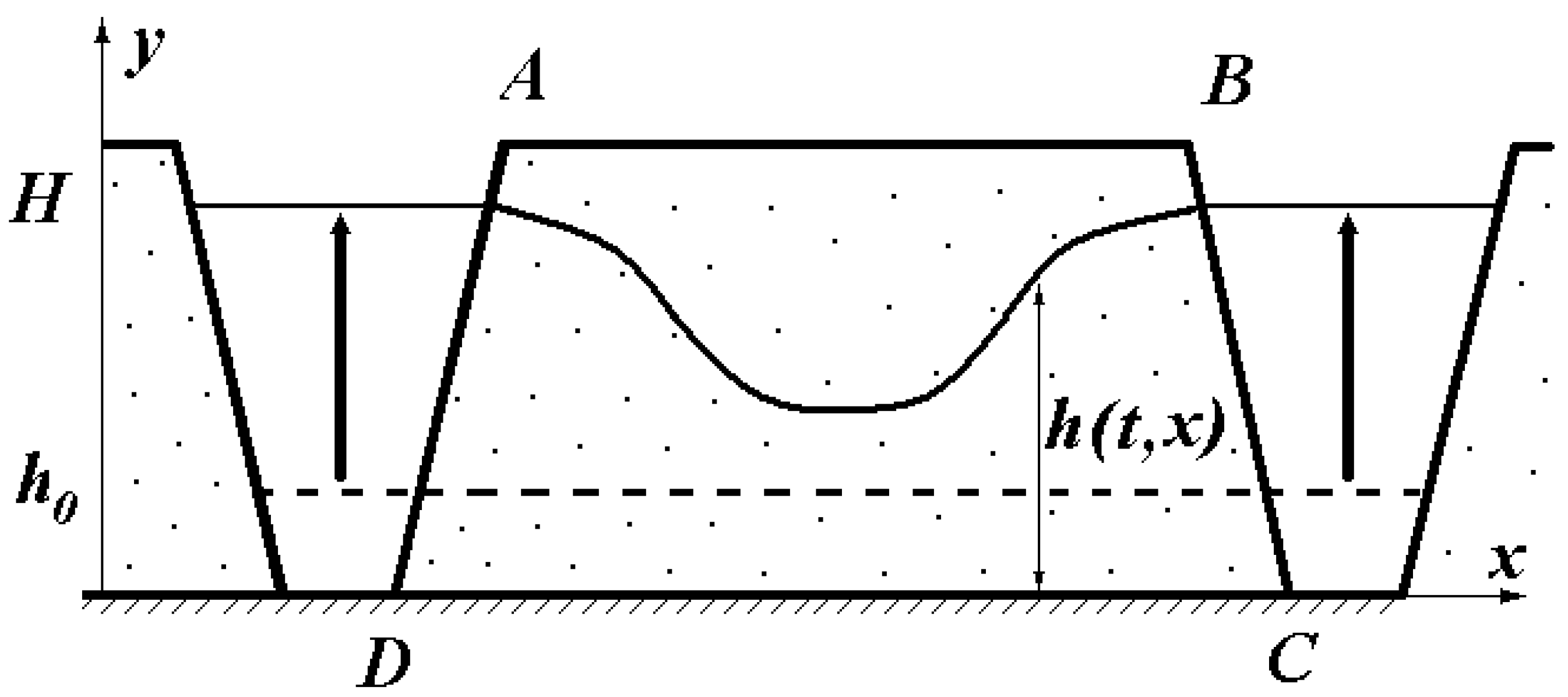
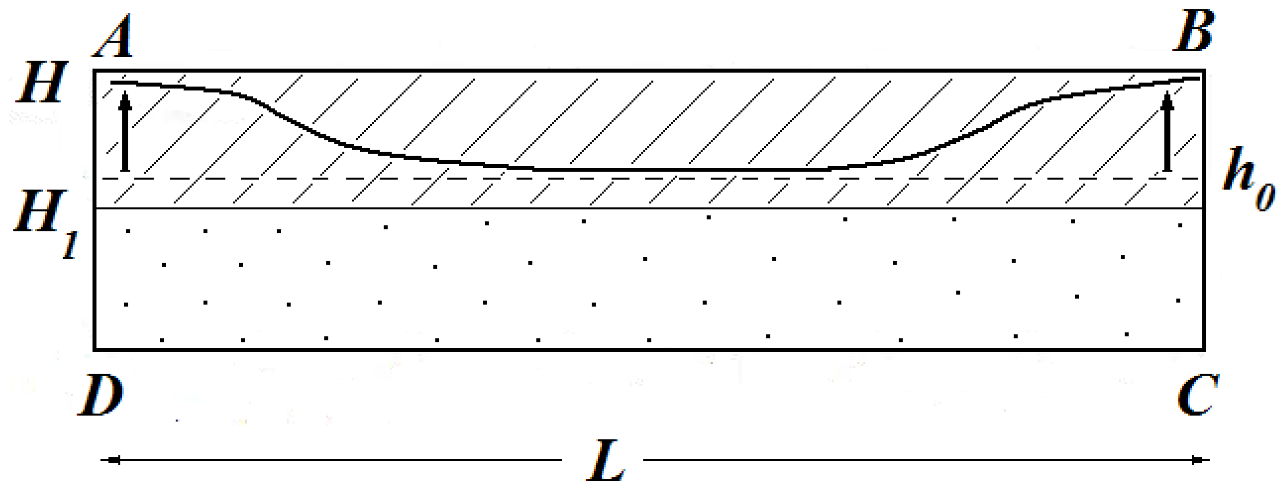
Here, we give a proof of the statement claimed in Section 2.2 that the solution $h(t,x)$ to the inundation problem in Equations (2)–(4) with an arbitrary distribution of hydraulic conductivity $K(x,y)$ in the domain $ABCD$ is monotonous with respect to K for sufficiently large t. Clearly, at large times, the solution approaches equilibrium, in which $h\equiv H$ and $u\equiv H$. Near the equilibrium state, we introduce new sought variables, $V(t,x)=H-h(t,x)$ and $U(t,x,y)=u(t,x,y)-H$, and linearize the problem in Equations (2)–(4) with respect to them. In the linearized problem, the upper boundary of the flow domain is fixed and coincides with the horizontal segment of the line $y=H$ between its intersection points with the lateral boundaries of $ABCD$. In the new variables, the problem can be written as

$$q=-K(x,y)\nabla U,\nabla ·q=0\mathrm{for}0<y<H$$

(13)

with boundary conditions

$$U(t,x,y)=0\mathrm{on}AC\mathrm{and}BC\mathrm{at}0<y<H,$$

(14)

$$U(t,x,H)=-V(t,x),$$

(15)

$$q_y=0\mathrm{at}y=0,$$

(16)

$$m(x,H)\frac{\partial V}{\partial t}=-q_y\mathrm{at}y=H.$$

(17)

Given the function $V(t,x)$ on the upper boundary of the linearized flow domain, the mixed-type boundary conditions in Equations (14)–(16) are sufficient to solve linear Equation (13). The existence and uniqueness of such solution is guaranteed for any function $V(t,x)$ which is continuous with respect to x and takes zero values at the ends of the upper boundary of the flow domain. This solution is linearly dependent on $V(t,x)$. Accordingly, the vertical component of the flow $q_y$ at the upper boundary of the domain can be uniquely determined by $V(t,x)$. Thus, a linear nonlocal operator $V\to A\left(V\right)$ is defined, transforming an arbitrary function $V=V(t,x)$ into a function $q_y(t,x,H)$ via the solution of the boundary value problem in Equations (13)–(16). In the mathematical literature, this operator is called after Lyapunov. Now, the remaining Equation (17) becomes $m\partial V/\partial t=-A\left(V\right)$.

As $q_y(t,x,H)$ depends on time only via function $V(t,x)$, the linear operator $A(·)$ does not depend on time. Therefore, the non-stationary Equation (17) can be solved by Fourier method, by expanding its solution as a series in the eigenfunctions of the spectral problem

$$\lambda mV=A\left(V\right).$$

(18)

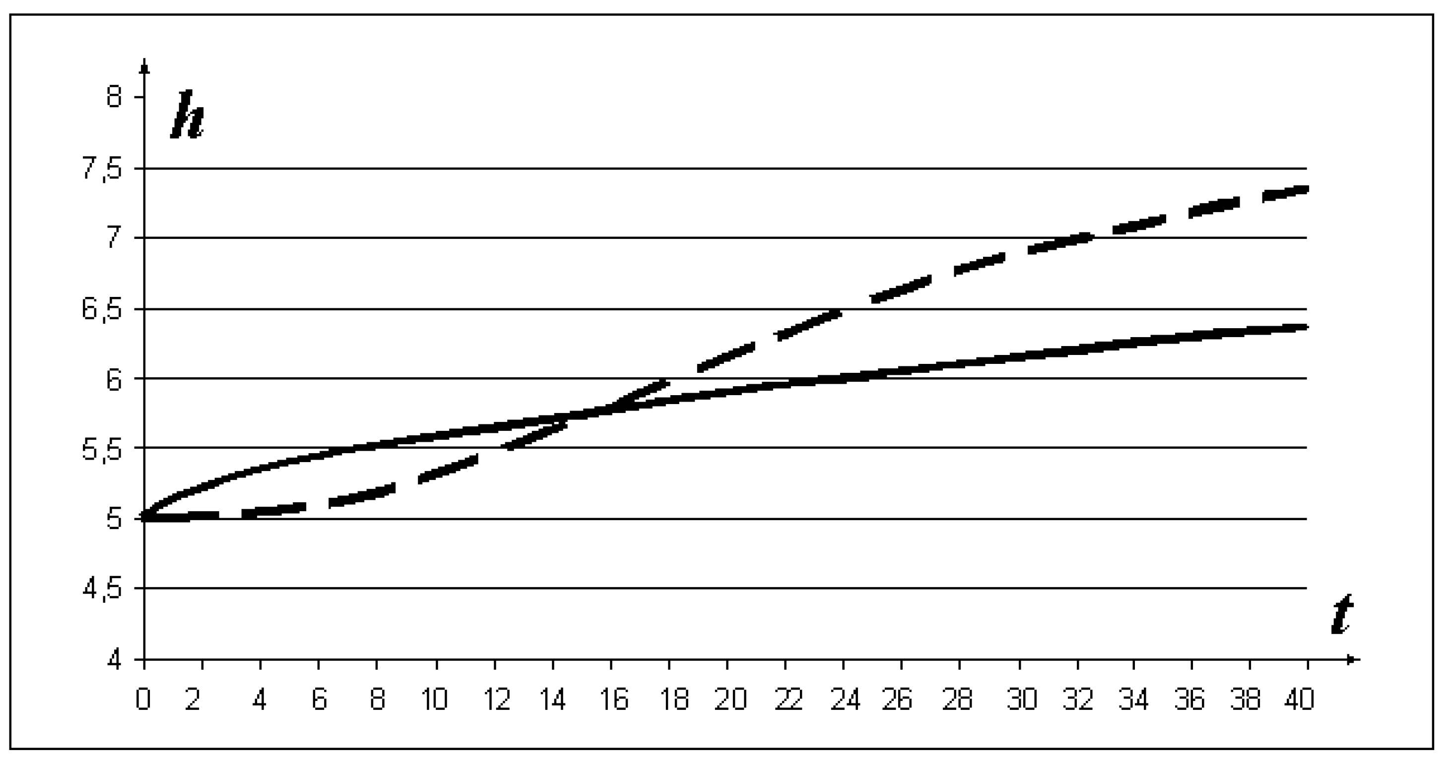
The properties of Lyapunov operator spectrum are well known (see, eg., [20]). This operator is self-adjoint, and the problem in Equation (18) has a countable set of real eigenvalues $\lambda ={\lambda }_N$, $N=1,2,\dots$, $0<{\lambda }_1\le {\lambda }_2\le {\lambda }_3\le \dots$, and corresponding eigenfunctions $V=V_N\left(x\right)$, which form a basis in the space of square integrable functions. Therefore, the solution of Equation (17) can be given as

$$V(t,x)=H-h(t,x)=\sum _{N=1}^{\infty }{C}_N{e}^{-{\lambda }_{N}t}{V}_N\left(x\right)$$

(19)

where $C_N$ are some constants, determined by the initial conditions. All terms of this series exponentially tend to zero at $t\to \infty$, although with different rates. Clearly, at large time, the main contribution to $V(t,x)$ is due to the longest-living among these terms, which corresponds to the least ${\lambda }_N$. The first eigenvalue ${\lambda }_1$ of the Lyapunov operator is known to be simple, so ${\lambda }_1<{\lambda }_2$, and the corresponding eigenfunction has a constant sign all over the interval of x. Therefore, $C_1\ne 0$, because the level of $y=h(t,x)$ at any time moment lies below the value of H.

In the case of arbitrary distribution of parameters, the least eigenvalue ${\lambda }_1$ cannot be calculated, although some variational estimates can be obtained for it. For the least eigenvalue of the self-adjoint operator and the corresponding eigenfuction, the Rayleigh principle holds in the following form:

$${\lambda }_1=\underset{V}{min}\left(\int A(V)Vdx\right){\left(\int m(x,H)V^2(x)dx\right)}^{-1}$$

(20)

where integrals are calculated along the horizontal segment of the line $y=H$ between its intersection points with the lateral boundaries of domain $ABCD$, and the minimum is taken over all functions $V\left(x\right)$ from the domain of definition of operator $A(·)$, which are not identically zero. The minimum is attained at $V=V_1\left(x\right)$. A variation formulation also exists for the two-dimensional problem in Equations (13)–(16) in the flow domain. In accordance with Dirichlet principle, its solution minimizes the expression

$$I(U)=\int \int K\nabla U·\nabla Udxdy$$

over all functions $U=U(x,y)$ with square integrable gradient, which satisfy the boundary conditions in Equations (14) and (15). The remaining boundary condition on the aquiclude in Equation (16) and Equation (13) are satisfied in the flow domain for the function that minimizes this expression, and these conditions are necessary for the existence of extremum. In the minimum, i.e., for the solution of the problem in Equations (13)–(16), the expression for $I\left(U\right)$ can be reduced by integration by parts to become

$$\int {\left(K\nabla U\right)}_y{U|}_{y=H}dx=\int A\left(V\right)Vdx$$

because $U=-V$ and ${(K\nabla U)}_y=-q_y$ at $y=H$. As a result, the Rayleigh principle (Equation (20)) takes the form

$${\lambda }_1=\underset{U}{min}\left(\int \int K\nabla U·\nabla Udxdy\right){\left(\int m(x,H)U^2(x,H)dx\right)}^{-1}$$

where the minimum is taken over all functions $U=U(x,y)$ that satisfy the boundary conditions in Equation (14) on the lateral sides of the flow domain and are not identically zero.

The obtained expression is convenient to construct estimates for the eigenvalue ${\lambda }_1$ and, therefore, for the principal term of the asymptotic at $t\to \infty$ of the solution $h=h(t,x)$ to the problem of level recovery in Equations (2)–(4), as this expression monotonically depends on the distribution of the tensor of hydraulic conductivity $K(x,y)$. Indeed, for any fixed function $U=U(x,y)$, the greater is right-hand part of this expression, the greater is $K(x,y)$. Therefore, the minimal value ${\lambda }_1$ of this expression over all possible functions $U(x,y)$ has the appropriate monotonicity properties. If $K_0(x,y)$ and $K_1(x,y)$ are two different distributions of the hydraulic conductivity tensor, and $K_0(x,y)<K_1(x,y)$, then the last variation equality yields the relationship ${\lambda }_1^{\left(0\right)}<{\lambda }_1^{\left(1\right)}$ for the respective eigenvalues. Now, from the presentation of the solution in Fourier series (Equation (19)), we have the inequality $h^{\left(0\right)}(t,x)<h^{\left(1\right)}(t,x)$ for sufficiently large t, which was to be proved.

4. Conclusions

The rigorous analysis of two groundwater flow problems has shown that the dependence of the solutions on the permeability distribution in porous media can be quite different from intuitively obvious expectations. It has been proved that, in the problem of groundwater inflow into an open reservoir, the rule “the greater the hydraulic conductivity, the greater the inflow” holds true only in particular cases, for example, for homogeneous aquifers. In general, the engineering estimates that are based on this rule require more careful argumentation. In addition, it has been demonstrated that the rate of groundwater level response to changes in boundary conditions may depend non-monotonically on hydraulic conductivity. For instance, at the initial stage of the inundation process, the free boundary may rise faster in a medium with lower conductivity.

On the other hand, in many cases, the dependence of solutions on permeability turns out to be in a good qualitative agreement with intuitive assumptions. However, a rigorous mathematical justification of these assumptions can be non-trivial. In particular, for the problem of groundwater inflow into an open reservoir, it is shown that the rate of inflow is monotone with respect to transmissivity distribution if the groundwater head at the external boundary of the flow domain is constant. In addition, it is proved that, for the inundation problem in a heterogeneous aquifer, the heuristic rule “the greater the soil permeability, the faster the water level rise” holds true for the long-time behavior of the solution.

References

1. Rajabi, M.M.; Ataie-Ashtiani, B.; Simmons, C.T. Model-data interaction in groundwater studies: Review of methods, applications and future directions. J. Hydrol. 2018, 567, 457–477. [Google Scholar] [CrossRef]
2. Sobol, I.M. Global sensitivity indices for nonlinear mathematical models and their Monte Carlo estimates. Math. Comput. Simul. 2001, 55, 271–280. [Google Scholar] [CrossRef]
3. Fajraoui, N.; Fahs, M.; Younes, A.; Sudret, B. Analyzing natural convection in porous enclosure with polynomial chaos expansions: Effect of thermal dispersion, anisotropic permeability and heterogeneity. Int. J. Heat Mass Transf. 2017, 115, 205–224. [Google Scholar] [CrossRef]
4. Krasnoselskii, M.F. Positive Solutions of Operator Equations; Nordhoff: Groningen, The Netherlands, 1964. [Google Scholar]
5. Duvaut, G.; Lions, J.-L. Les Inéquations en Méchanique et en Physique; DUNOD: Paris, France, 1972. [Google Scholar]
6. Friedman, A. Partial Differential Equations of Parabolic Type; Prentice-Hall: Englewood Cliffs, NJ, USA, 1964. [Google Scholar]
7. Polubarinova-Koch, P.Y. Theory of Ground Water Movement; Princeton University Press: Princeton, NJ, USA, 1962. [Google Scholar]
8. Bear, J.; Zaslavsky, D.; Irmay, S. Physical Principles of Water Percolation and Seepage; UNESCO: Paris, France, 1968. [Google Scholar]
9. Torelli, A. On a free boundary value problem connected with a non steady filtration phenomenon. Ann. Sc. Norm. Super. Pisa-Cl. Sci. 1977, 4, 33–59. [Google Scholar]
10. Chipot, M. Variational Inequalities and Flow through Porous Media; Springer: New York, NY, USA, 1984. [Google Scholar]
11. Belyaev, A.I.; Yushmanov, I.O. A variational principle for problems of steady-state groundwater flow with free surface. Fluid Dyn. 2015, 50, 543–557. [Google Scholar] [CrossRef]
12. Brézis, H.; Kinderlehrer, D.; Stampacchia, G. Sur une nouvelle formulation du problème d’éqoulement à travers une digue. C. R. Acad. Sci. Paris Ser. A 1978, 287, 711–714. [Google Scholar]
13. Alt, H.W. Strömungen durch inhomogene poröse Medien mit freiem Rand. J. Reine Angew. Math. 1979, 305, 89–115. [Google Scholar]
14. Beliaev, A.Y. Solvability of free boundary problems for steady groundwater flow. Eur. J. Appl. Math. 2015, 26, 821–847. [Google Scholar] [CrossRef]
15. Girinskii, N.K. Some problems in groundwater dynamics. Hydrogeol. Geotech. Eng. Coll. Pap. VSEGINGEO 1947, 9, 27–32. (In Russian) [Google Scholar]
16. Myatiev, A.N. Confined aquifer system and wells. Izv. Akad. Nauk SSSR Otd. Tekh. Nauk 1947, 9, 1069–1088. (In Russian) [Google Scholar]
17. Manukyan, D.A. Hydrodynamic substantiation of a double-regulation system of water regime in peat bogs. In Proc. Intern. Conf. "Development Problems of Amelioration and Water Management and Ways to Their Solution. Part II “Integrated Development of Landscapes”; Moscow State University Prirodoustr.: Moscow, Russia, 2011; pp. 66–74. (In Russian) [Google Scholar]
18. Jikov, V.V.; Kozlov, S.M.; Oleinik, O.A. Homogenization of Differential Equations and Integral Functionals; Springer: Berlin, Germany, 1994. [Google Scholar]
19. Belyaev, A.Y.; Kozlov, S.M. Hierarchical structures and estimates for homogenized coefficients. Russ. J. Math. Phys. 1992, 1, 5–18. [Google Scholar]
20. Sadovnichii, V.A.; Chechkina, A.G. On estimate of eigenfunctions of the Steklov-type problem with a small parameter in the case of a limit spectrum degeneration. Ufa Math. J. 2011, 3, 122–134. [Google Scholar]
Figure 1. Illustration to the problem of groundwater discharge from a confined aquifer into an open water body.
Fluids 03 00102 g001
Figure 2. Cross-section of the flow domain in the problem of water rise in an unconfined aquifer.
Fluids 03 00102 g002
Figure 3. Cross-section of the flow domain in the problem of inundation of a layered aquifer system.
Fluids 03 00102 g003
Figure 4. Recovery dynamics of groundwater level (h, m) in the central point between canals over time (t, day) in media with a homogeneous (dashed curve) and a heterogeneous (solid curve) structure.
Fluids 03 00102 g004