A Hybrid Analytics Paradigm Combining Physics-Based Modeling and Data-Driven Modeling to Accelerate Incompressible Flow Solvers

Abstract

Numerical solution of the incompressible Navier–Stokes equations poses a significant computational challenge due to the solenoidal velocity field constraint. In most computational modeling frameworks, this divergence-free constraint requires the solution of a Poisson equation at every step of the underlying time integration algorithm, which constitutes the major component of the computational expense. In this study, we propose a hybrid analytics procedure combining a data-driven approach with a physics-based simulation technique to accelerate the computation of incompressible flows. In our approach, proper orthogonal basis functions are generated to be used in solving the Poisson equation in a reduced order space. Since the time integration of the advection–diffusion equation part of the physics-based model is computationally inexpensive in a typical incompressible flow solver, it is retained in the full order space to represent the dynamics more accurately. Encoder and decoder interface conditions are provided by incorporating the elliptic constraint along with the data exchange between the full order and reduced order spaces. We investigate the feasibility of the proposed method by solving the Taylor–Green vortex decaying problem, and it is found that a remarkable speed-up can be achieved while retaining a similar accuracy with respect to the full order model.

1. Introduction

In the latest age of digitalization, industries demand technologies and algorithms that would make near real-time predictions, control and monitoring in the context of Digital Twin a possibility. A Digital Twin [1] may be defined as: the virtual representation of a physical object or system across its lifecycle, using real-time data and other sources to enable understanding, learning, reasoning, and dynamic recalibration for improved decision-making. Until recently, purely data-driven artificial intelligence and machine learning algorithms were looked upon as the most attractive enabling technologies for Digital Twins. However, owing to their blackbox nature, they have not yet found whole-hearted acceptance within the engineering community specially in critical applications. This has led to the development of a new field of research called the “Hybrid Analytics” that combines the interpretability, robust foundation and understanding of a physics-based modeling approach with the accuracy, computational efficiency, and automatic pattern-identification capabilities of advanced data-driven machine learning and artificial intelligence algorithms. The current work is an effort to demonstrate one way of conducting hybrid analytics involving a combination of an unsupervised machine learning algorithm called the proper orthogonal decomposition and a set of physics-based governing equations describing incompressible flows, of either gases or liquids, including a wide range of subjects in basic scientific and engineering research such as wind energy, hydrodynamics, heat and mass transfer, aerodynamics or biological fluid mechanics [2,3,4,5,6].

Incompressible flows are fluid flows in which density changes do not affect the flow physics, i.e., the effect of pressure on density is negligible [7]. Although the filtering of such acoustics modes simplifies the underlying physics, there are some computational difficulties in solving the incompressible flow equations since they become parabolic-elliptic in their nature. Therefore, there have been many successful algorithms proposed to advance incompressible flow computations, and computational study of incompressible flow is still an active research field [8,9,10]. One basic approach for solving incompressible flow problems is known as artificial compressibility or the density-based method, where the computation is performed using a compressible form of Navier–Stokes equations [11,12]. This approach usually requires using a smaller time step to satisfy the Courant–Friedrichs–Lewy (CFL) criterion for explicit time integration procedures. For example, if the average flow field Mach number is $0.05$, then the time step for the density-based incompressible flow solver has to be approximately 20 times smaller than other flow solvers that use a primitive incompressible flow formulation.

Another widely used approach is the pressure-based method where the density is treated as constant in the entire flow domain. The challenging part in the modeling of the incompressible flows using a pressure-based approach is to find an appropriate equation to calculate a pressure field since the equation of state can not be used if the density is considered as a constant [13]. As a result, a Poisson equation is used to find the pressure field (or augmented pressure-like field) and the pressure–velocity coupling is done by satisfying the continuity equation or mass conservation. A large variety of solution techniques are developed based on the pressure-based method framework such as a projection algorithm for the primitive variable formulation [14,15], the vorticity-stream function formulation [16,17], the explicit pressure Poisson equation solution technique (compact schemes [18], non-compact schemes [19], staggered grid arrangements [20], collocated grid arrangements [21], momentum interpolation techniques [22]), the implicit pressure Poisson equation solution technique (sequential methods [23], operator splitting methods [24], fractional step methods [25,26], marker and cell methods [27], SIMPLE methods [28], Pressure-Implicit with Splitting of Operators (PISO) methods [29]), etc. Solving the pressure Poisson equation is also computationally costly since it is the most time-consuming part of the solver as well as having to be solved multiple times in each time step if a multi-stage solver is used. In the present study, we use the vorticity-stream function formulation approach for our physics-based full order modeling simulations to put forth a hybrid analytic framework combining this full order model with a data-driven technique.

Due to increasing demand on computational efficiency for simulating complex and large-scale dynamical systems, and limitation of computational resources to obtain high-fidelity simulations, there has been a substantial effort aimed at generating lower dimensional systems with a similar range of accuracy and validity. Model order reduction or reduced order modeling (ROM) is such a framework that replaces the large dimensional system with a lower dimensional one having a significant reduction in computational costs [30,31,32,33,34]. An overview of some of the widely used ROM techniques can be found in [35]. There is also a growing interest in developing machine learning methods for model order reduction in fluids [36,37,38,39,40,41,42,43]. In our study, we have used the proper orthogonal decomposition (POD) framework coupled with the Galerkin projection, which is considered an efficient approach to generate ROMs for nonlinear systems [44,45,46]. The POD approach has been applied in a large number of problems involving fluids over the past few decades [47,48,49] where the most energetic modes (POD modes) of a given dataset are extracted to generate a reduced order system [50]. Other insignificant modes are excluded assuming that the selected POD modes capture the dominant characteristics of the system. The dataset to obtain POD basis functions can be generated from a high-fidelity experiment or numerical simulation of a large dimensional system. In addition, the POD modes can be generated based on the dataset obtained by an initial simulation or experimental data. However, similar to the other data-driven methodologies, POD modes cannot capture any physics outside of the given dataset. In our study, we have developed a POD-based ROM approach to accelerate the Poisson solver part of the pressure-based incompressible flow solvers.

Apart from the model order reduction approach, there are a considerable number of approaches that have been proposed to accelerate the incompressible flow solvers. For example, the coarse-grid projection (CGP) method reduces the number of grid points of the elliptic solver, which is the most time-consuming part of the problem to accelerate the flow simulation [51]. The CGP framework was initially proposed by Lentine et al. [52] for real-time visual simulation of computer games. Later, more developments have been made on this CGP methodology through several studies over the years [53,54,55]. Another common approach to decrease the computational expense of incompressible flow solvers is the implementation of robust multigrid (MG) solvers [56,57,58,59,60]. For an orthogonal coordinate grid system or certain ideal problems on equally-spaced grids, a fast Fourier transform (FFT)-based fast Poisson solver (FPS) is considered the fastest algorithm for solving Poisson equations [61]. We refer Ref.[53] to get a comparative analysis on the computational efficiency of these Poisson solvers along with the traditional iterative solvers. Furthermore, with the advancement of computational resources through graphics processing units (GPU), the incompressible flow simulations can be accelerated [62,63]. Indeed, these GPU based approaches can be easily incorporated in our proposed approach due to the parallelism simplicity of the advection–diffusion part.

The main objective of this paper is to develop a novel hybrid analytics approach combining physics-based models with the data-driven reduced order models, which will contribute a firm unified foundation for the computational modeling and simulation of incompressible flow problems. Solving the elliptical equation in most of the pressure-based solvers is the main contributor of the overall computational cost when such incompressible flows are simulated. Even though there are a number of elliptic equation algorithms developed with a goal to accelerate the incompressible flow simulations, the numerical solution of the Poisson equation is still the most time-consuming part with respect to the advection–diffusion update [64,65,66]. Moreover, some of these advanced approaches are too complicated to implement in a generalized way, and also limited to certain conditions. In our hybrid analytics ROM (HA-ROM), we compute the Poisson equation in reduced order space to accelerate the flow simulation and solve the non-stiff advective-diffusive part in full order space to retain the accuracy. An encoder and decoder approach is utilized for the data exchange between the full order space and reduced order space. By implementing the hybrid analytics framework, significant savings in computational time are found with little compromise in the accuracy of the solutions since the computations in reduced order space lose some negligible amount of accuracy. Furthermore, it is found that the hybrid analytic framework not only accelerates the incompressible flow solver, but also reduces much of the computational complexities in solving Poisson equation by precomputing the basis function and ROM coefficient before the start of online computation. To assess the idea, we consider two simple numerical test cases and compare the obtained hybrid analytics solution with the full-order simulation solution as well as with the analytical solution.

The rest of the paper is structured as follows. Section 2 provides the mathematical models including the governing equations for incompressible flow in terms of the primitive variables fractional step and vorticity-stream function formulations. The proposed hybrid analytics approach is introduced and illustrated in Section 3 along with a detailed description of physics-based modeling and data-driven modeling. The respective flow solver algorithms are also presented and described in the subsections. In Section 4, the hybrid analytics framework is applied to the numerical test problems and our results are presented for solving the Taylor–Green vortex decaying problem. The results are also compared with the analytical solution and the full order model solution in this section. Finally, the summary of the other sections is presented as well as the conclusions drawn based on the results in Section 5.

2. Mathematical Modeling of Incompressible Flows

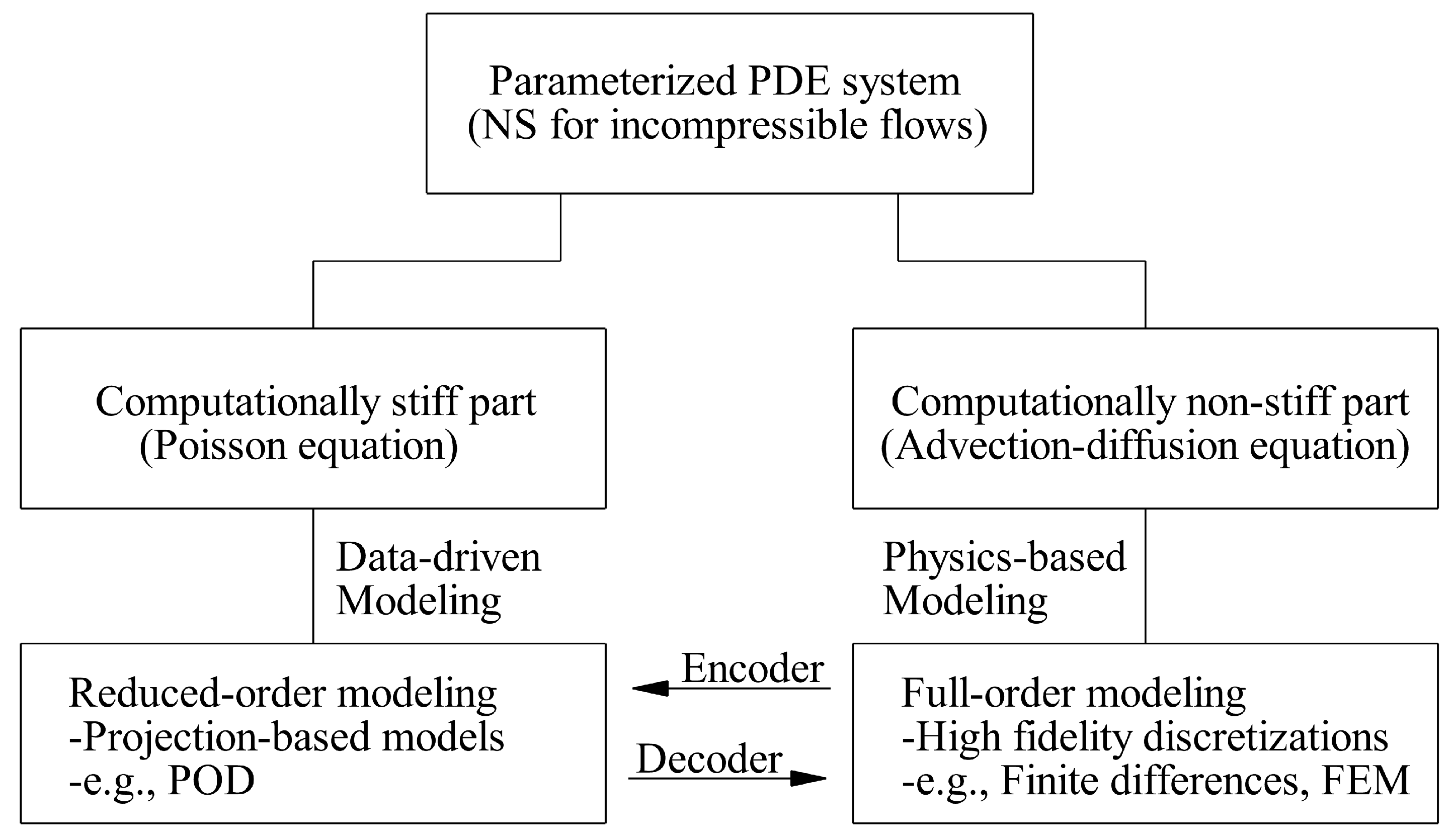
The governing equations for unsteady two-dimensional incompressible flows in terms of primitive variables, velocity $\mathbf{u}$ and pressure p can be written in a dimensionless form as

$$\begin{array}{cc}\hfill & \nabla ·\mathbf{u}=0,\hfill \end{array}$$

(1)

$$\begin{array}{c}\frac{\partial \mathbf{u}}{\partial t}+\mathbf{u}·\nabla \mathbf{u}=-\nabla p+\frac{1}{Re}{\nabla }^2\mathbf{u},\hfill \end{array}$$

(2)

where $Re$ is the Reynolds number and p is the non-dimensional pressure variable. To illustrate the physics-based modeling, we have used the fractional step method, also referred to as a time-splitting or projection method [67,68,69]. This is an implicit approach to ensure divergence free evolution of velocity field for incompressible Navier–Stokes equations. In this approach, the solution procedure of momentum equation is split into the predictor step, pressure correction step and the projection step. The first step is called the predictor step, in which the advection–diffusion equation is solved to estimate the velocity field. The advection–diffusion equation can be obtained by excluding the pressure gradient term from the momentum equation and can be expressed as

$$\begin{array}{c}\hfill \frac{\partial \tilde{\mathbf{u}}}{\partial t}+\tilde{\mathbf{u}}·\nabla \tilde{\mathbf{u}}=\frac{1}{Re}{\nabla }^2\tilde{\mathbf{u}}.\end{array}$$

(3)

The second step is the pressure correction step where a pressure Poisson equation is solved. The pressure Poisson equation is formed using the intermediate velocity field $\tilde{\mathbf{u}}$ obtained by solving the advection–diffusion equation and can be written as follows:

$$\begin{array}{c}\hfill {\nabla }^{2}p=\frac{1}{\Delta t}(\nabla ·\tilde{\mathbf{u}}).\end{array}$$

(4)

Finally, $\tilde{\mathbf{u}}$ is projected onto the divergence-free space in the projection step to obtain the corrected velocity field using the following equation:

$$\begin{array}{c}\hfill \mathbf{u}=\tilde{\mathbf{u}}-\Delta t(\nabla p).\end{array}$$

(5)

A state-of-the-art algorithm for a predictor–corrector type of fractional step method can be found in Ref. [70]. On the other hand, the vorticity-stream function formulation can also be used to solve the incompressible flow problems that eliminates the projection inaccuracies observed in the fractional step formulation using primitive variables [14]. In terms of the hybrid analytics framework proposed in this study, we can consider either a vorticity-stream function method or primitive equation fractional step method since both of them require solutions of an elliptic equation with each time step. For two-dimensional flows, it is more beneficial to use vorticity-stream function formulation in a sense that it is free of odd–even decoupling (checkerboard patterning issue) while satisfying the mass conservation by eliminating the pressure from governing equations as well as the number of equations to be solved being reduced [71]. By taking the curl of the momentum equations of the Navier–Stokes equation, the dimensionless form of the governing equations can be written as

$$\begin{array}{ccc}\frac{\partial \mathit{\omega }}{\partial t}+\mathbf{u}·\nabla \mathit{\omega }=\mathit{\omega }·\nabla \mathbf{u}+\frac{1}{Re}{\nabla }^2\mathit{\omega },& \mathrm{and}& {\nabla }^2\mathbf{u}=-\nabla \times \mathit{\omega }\end{array}$$

(6)

where $\mathit{\omega }$ is the kinematic vorticity field, defined as

$$\begin{array}{c}\hfill \mathit{\omega }=\nabla \times \mathbf{u}.\end{array}$$

(7)

For two-dimensional flow in the x-y plane, i.e., $\mathit{\omega }=(0\widehat{i},0\widehat{j},\omega \widehat{k})$, the z component of the vorticity field becomes

$$\begin{array}{c}\hfill \omega =\frac{\partial v}{\partial x}-\frac{\partial u}{\partial y}.\end{array}$$

(8)

The flow velocity components can be found from the stream function $\psi$ using the following definition:

$$\begin{array}{c}\hfill \mathbf{u}=\nabla \times \psi \widehat{k}.\end{array}$$

(9)

In Cartesian coordinates,

$$\begin{array}{c}\hfill u=\frac{\partial \psi }{\partial y},v=-\frac{\partial \psi }{\partial x}.\end{array}$$

(10)

The kinematic equation connecting the vorticity and stream function can be found by substituting the velocity components in terms of stream function in Equation (8), which forms the following Poisson equation:

$$\begin{array}{c}\hfill {\nabla }^2\psi =-\omega .\end{array}$$

(11)

Putting the definitions of velocity components in terms of stream function and vorticity from Equations (8) and (10), respectively, in Equation (6), we get

$$\begin{array}{c}\hfill \frac{\partial \omega }{\partial t}+J(\omega ,\psi )=\frac{1}{Re}\left(\frac{{\partial }^2\omega }{\partial x^2}+\frac{{\partial }^2\omega }{\partial y^2}\right),\end{array}$$

(12)

where $J(\omega ,\psi )$ is the nonlinear Jacobian, defined as

$$\begin{array}{c}\hfill J(\omega ,\psi )=\frac{\partial \psi }{\partial y}\frac{\partial \omega }{\partial x}-\frac{\partial \psi }{\partial x}\frac{\partial \omega }{\partial y}.\end{array}$$

(13)

In our study, we have used the vorticity-stream function formulation to illustrate the idea because of its advantages over the primitive variables formulation for two-dimensional flows. The numerical modeling of the above formulation will be discussed in Section 3.1.

3. Hybrid Analytics

The proposed hybrid analytics approach can be applied to any parameterized partial differential equation (PDE) system (in our case, two-dimensional Navier–Stokes equations for incompressible flows) which combines a full order treatment for the computationally non-stiff part of the problem with an optimized reduced order treatment for the stiff time-consuming part to generate a more efficient and robust solution. In general, the Poisson equation solver is the computationally stiff part of an incompressible flow solver, i.e., it occupies the majority percentage of the overall computational costs, whereas the advection–diffusion solver is the computationally non-stiff part. For example, the computational cost of the Poisson equation part in a Gauss–Seidel iteration based incompressible flow solver is $O\left(N^2\right)$ and the computational cost of the advection–diffusion part is $O\left(N\right)$. Here, N is the total number of the degrees of freedom in a two-dimensional system. Even though there are some optimal Poisson solvers available to accelerate the overall flow simulation (e.g., $O\left(N\log N\right)$ for FPS), it is found that the computational cost is still higher for the Poisson equation solver [53]. In a hybrid analytics framework of an incompressible flow solver, we compute the elliptic Poisson equation in the reduced order space using any ROM architecture (like POD) so that the ROM coefficients and POD basis functions can be precomputed before the time iteration starts. As a result, the only thing that needs to be updated in the Poisson equation at each time step is the modal coefficients of the ROM. The details about the reduced order modeling framework will be presented in Section 3.2. On the other hand, we need the updated vorticity field data from full order model (FOM) to compute the modal coefficients in reduced order space, and then the updated modal coefficients data are sent to the full order space to update the stream function field. This data transfer between full order space and reduced order space is done by an encoder and decoder approach. The proposed hybrid analytics reduced order modeling approach to accelerate incompressible flow solvers will be detailed in Section 3.3. As shown in Figure 1, our hybrid analytics framework can be summarized as follows:

• Identify computationally stiff and non-stiff parts of the problem,
• Build a data-driven model to solve the stiff part efficiently,
• Establish encoder and decoder approaches for data transfer between the stiff and non-stiff sub-problems.

3.1. Physics-Based Modeling

We do all the computations in full order space for the physics-based modeling. The spatial discretization of the partial differential equations (PDEs) given by Equation (12) leads to a system of coupled ordinary differential equations (ODEs) in the following simplified form:

$$\begin{array}{c}\hfill \frac{d{\omega }_{i,j}}{dt}=R_{i,j},\end{array}$$

(14)

where R denotes the discrete expression of spatial derivative operator including the nonlinear convective terms and the linear diffusive terms. We use the finite difference approximation to discretize the Equation (14) as

$$\begin{array}{c}\hfill {\omega }_{i,j}^{n+1}={\omega }_{i,j}^n+\Delta t{R}_{i,j}^n.\end{array}$$

(15)

Here, the right-hand side can be expressed by $R_{i,j}^n=-J({\omega }_{i,j}^n,{\psi }_{i,j}^n)+\frac{1}{Re}{\nabla }^2{\omega }_{i,j}^n$ for the Euler scheme. To avoid computational instabilities arising from nonlinear interactions, we use second-order skew-symmetric, energy and enstrophy conserving Arakawa scheme for the nonlinear Jacobian [17]. The Jacobian defined in Equation (13) can be expressed as

$$\begin{array}{c}\hfill J({\omega }_{i,j},{\psi }_{i,j})=\frac{1}{3}(J_1({\omega }_{i,j},{\psi }_{i,j})+J_2({\omega }_{i,j},{\psi }_{i,j})+J_3({\omega }_{i,j},{\psi }_{i,j})),\end{array}$$

(16)

where

$$\begin{array}{cc}\hfill J_1({\omega }_{i,j},{\psi }_{i,j})=& \frac{1}{4\Delta x\Delta y}[({\omega }_{i+1,j}-{\omega }_{i-1,j})({\psi }_{i,j+1}-{\psi }_{i,j-1})\hfill \\ & -({\omega }_{i,j+1}-{\omega }_{i,j-1})({\psi }_{i+1,j}-{\psi }_{i-1,j})],\hfill \end{array}$$

(17)

$$\begin{array}{cc}\hfill J_2({\omega }_{i,j},{\psi }_{i,j})=& \frac{1}{4\Delta x\Delta y}[{\omega }_{i+1,j}({\psi }_{i+1,j+1}-{\psi }_{i+1,j-1})-{\omega }_{i-1,j}({\psi }_{i-1,j+1}-{\psi }_{i-1,j-1})\hfill \\ & -{\omega }_{i,j+1}({\psi }_{i+1,j+1}-{\psi }_{i-1,j+1})-{\omega }_{i,j-1}({\psi }_{i+1,j-1}-{\psi }_{i-1,j-1})],\hfill \end{array}$$

(18)

$$\begin{array}{cc}\hfill J_3({\omega }_{i,j},{\psi }_{i,j})=& \frac{1}{4\Delta x\Delta y}[{\omega }_{i+1,j+1}({\psi }_{i,j+1}-{\psi }_{i+1,j})-{\omega }_{i-1,j-1}({\psi }_{i-1,j}-{\psi }_{i,j-1})\hfill \\ & -{\omega }_{i-1,j+1}({\psi }_{i,j+1}-{\psi }_{i-1,j})-{\omega }_{i+1,j-1}({\psi }_{i+1,j}-{\psi }_{i,j-1})].\hfill \end{array}$$

(19)

Here, $\Delta x$ and $\Delta y$ are the step size in x- and y-directions, respectively. We refer to Ref. [46] to find the detailed derivation of higher order Arakawa schemes. We also noted that we can simply use $J({\omega }_{i,j},{\psi }_{i,j})=J_1({\omega }_{i,j},{\psi }_{i,j})$ in our study, since the utilization of the energy conserving Arakawa scheme wouldn’t be that critical for solving the Taylor–Green vortex decaying problem presented in Section 4.2. For the time advancement in Equation (14), we have employed an optimal third-order-accurate total variation diminishing Runge–Kutta (TVDRK3) scheme [72]. The TVDRK3 scheme has been commonly used for the solution of hyperbolic conservation laws with the presence of nonlinearities [73,74]. Starting from the given vorticity field, ${\omega }^{\left(n\right)}$, at the current time step, the steps to compute the vorticity at the next time step, ${\omega }^{(n+1)}$, are given in the algorithm below:

$$\begin{array}{cc}\hfill {\nabla }^2{\psi }^{\left(n\right)}& =-{\omega }^{\left(n\right)},\hfill \end{array}$$

(20)

$$\begin{array}{c}\hfill R^{\left(n\right)}=-J({\omega }^{\left(n\right)},{\psi }^{\left(n\right)})+\frac{1}{Re}{\nabla }^2{\omega }^{\left(n\right)},\end{array}$$

(21)

$$\begin{array}{c}\hfill {\omega }^{\left(1\right)}={\omega }^{\left(n\right)}+\Delta t{R}^{\left(n\right)},\end{array}$$

(22)

$$\begin{array}{c}\hfill {\nabla }^2{\psi }^{\left(1\right)}=-{\omega }^{\left(1\right)},\end{array}$$

(23)

$$\begin{array}{c}\hfill R^{\left(1\right)}=-J({\omega }^{\left(1\right)},{\psi }^{\left(1\right)})+\frac{1}{Re}{\nabla }^2{\omega }^{\left(1\right)},\end{array}$$

(24)

$$\begin{array}{c}\hfill {\omega }^{\left(2\right)}=\frac{3}{4}{\omega }^{\left(n\right)}+\frac{1}{4}{\omega }^{\left(1\right)}+\frac{1}{4}\Delta t{R}^{\left(1\right)},\end{array}$$

(25)

$$\begin{array}{c}\hfill {\nabla }^2{\psi }^{\left(2\right)}=-{\omega }^{\left(2\right)},\end{array}$$

(26)

$$\begin{array}{c}\hfill R^{\left(2\right)}=-J({\omega }^{\left(2\right)},{\psi }^{\left(2\right)})+\frac{1}{Re}{\nabla }^2{\omega }^{\left(2\right)},\end{array}$$

(27)

$$\begin{array}{c}\hfill {\omega }^{(n+1)}=\frac{1}{3}{\omega }^{\left(n\right)}+\frac{2}{3}{\omega }^{\left(2\right)}+\frac{2}{3}\Delta t{R}^{\left(2\right)}.\end{array}$$

(28)

The elliptic Poisson equation given by Equation (11) needs to be solved three times at every time step in the above formulation to update the vorticity field. In general, the common and simple iterative type of solvers (e.g., Richardson–Jacobi, alternating direction implicit (ADI), Gauss–Seidel (GS) or successive over relaxation (SOR)) are used to solve the Poisson equation, which can be upgraded to accelerate the performance using advanced numerical algorithms. In the current study, we have considered the Euler pseudo-time iteration approach during the computation of Poisson equation in our numerical test cases to present the idea without much computational complexities. This approach has also been used in the literature due to its straightforward extension while designing high-order computational schemes for incompressible flows [75]. To illustrate the pseudo-time iteration approach, we can write Equation (11) as

$$\begin{array}{c}\hfill \frac{\partial \psi }{\partial \tau }={\nabla }^2\psi +\omega ,\end{array}$$

(29)

where $\tau$ is the pseudo-time. The pseudo-time step will be advanced until $\frac{\partial \psi }{\partial \tau }\approx 0$ that means until the steady-state solution of $\psi$ is obtained. The discrete form of Equation (29) can be written as

$$\begin{array}{c}\hfill {\psi }_{i,j}^{m+1}={\psi }_{i,j}^m+\Delta \tau \left(r_{i,j}^m\right),\end{array}$$

(30)

where residual term

$$\begin{array}{c}\hfill r_{i,j}=\frac{{\psi }_{i+1,j}-2{\psi }_{i,j}+{\psi }_{i-1,j}}{\Delta x^2}+\frac{{\psi }_{i,j+1}-2{\psi }_{i,j}+{\psi }_{i,j-1}}{\Delta y^2}+{\omega }_{i,j}.\end{array}$$

(31)

Here, $\Delta x$ and $\Delta y$ are the grid spacing in x- and y-directions, respectively. From the von Neumann numerical stability criterion, the maximum pseudo-time increment $\Delta {\tau }_{max}$ can be found as

$$\begin{array}{c}\hfill \Delta {\tau }_{max}=\frac{1}{2(\frac{1}{\Delta x^2}+\frac{1}{\Delta y^2})}.\end{array}$$

(32)

Putting the $\Delta {\tau }_{max}$ in Equation (30), we get

$$\begin{array}{c}\hfill {\psi }_{i,j}^{m+1}={\psi }_{i,j}^m+\frac{1}{2\left(\frac{1}{\Delta x^2}+\frac{1}{\Delta y^2}\right)}\left(\frac{{\psi }_{i+1,j}^m-2{\psi }_{i,j}^m+{\psi }_{i-1,j}^m}{\Delta x^2}+\frac{{\psi }_{i,j+1}^m-2{\psi }_{i,j}^m+{\psi }_{i,j-1}^m}{\Delta y^2}+{\omega }_{i,j}\right).\end{array}$$

(33)

In our study, we use maximum available $\Delta \tau$ and equal grid spacing, i.e., $\Delta x=\Delta y=h$ which yields a scheme similar to the Richardson–Jacobi iterative method. We can write the following discrete Poisson equation for the Richardson–Jacobi iterative method using the second-order finite difference method for equal grid spacing:

$$\begin{array}{c}\hfill {\psi }_{i,j}^{m+1}=\frac{1}{4}({\psi }_{i+1,j}^m+{\psi }_{i-1,j}^m+{\psi }_{i,j+1}^m+{\psi }_{i,j-1}^m+h^2{\omega }_{i,j}).\end{array}$$

(34)

Putting $\Delta x=\Delta y=h$ in Equation (33), we get

$$\begin{array}{c}\hfill {\psi }_{i,j}^{m+1}={\psi }_{i,j}^k+\frac{1}{4}({\psi }_{i+1,j}^m+{\psi }_{i-1,j}^m+{\psi }_{i,j+1}^m+{\psi }_{i,j-1}^m-4{\psi }_{i,j}^m+h^2{\omega }_{i,j}).\end{array}$$

(35)

If we simplify Equation (35) further, we will find Equation (34) i.e., the Richardson–Jacobi equation.

3.2. Data-Driven Modeling

We have used a standard projection methodology in the data-driven modeling approach where a reduced order modeling framework is developed based on the stored sample solution of FOM in a data matrix, known as snapshots [76,77]. We utilize the POD model reduction framework, which is widely used in science and engineering applications with large dimensional systems of nonlinear ODEs or PDEs. The purpose behind the reduced order modeling approach is to reduce as well as represent a large dimensional system into a low-dimensional one by extracting the most energetic data sets or modes. This technique has a significant benefit in reducing the computational cost since the calculation is done in the reduced order space. The full order physics-based model is solved to generate and record the data snapshots for basis construction. The rest of the computations are built on these datasets. Hence, we denote this approach as a data-driven modeling approach. In our study, we solve the pressure Poisson equation given by the Equation (11) in reduced order space where we should compute $\psi$ from given $\omega$. To compute the POD basis functions, we first obtain Q number of snapshots for stream function field, $\psi$, by solving Equation (29) in full order space using a physics-based model. At pseudo-time $\tau ={\tau }_q$, the stream function field $\psi (x,y)$ can be denoted as $\psi (x,y,{\tau }_q)$ for $q=1,2,\dots ,Q$. A correlation matrix can be constructed from these snapshots data by

$$\begin{array}{c}\hfill {\alpha }_{ij}={\int }_{\Omega }\psi (x,y,{\tau }_i)\psi (x,y,{\tau }_j)dxdyx,y\in \Omega ,\end{array}$$

(36)

where $\Omega$ is the two-dimensional domain, and i and j refer to the snapshot indices. We can define the inner product of two functions $f=f(x,y)$ and $g=g(x,y)$ as

$$\begin{array}{c}\hfill \langle f,g\rangle ={\int }_{\Omega }f(x,y)g(x,y)dxdy,\end{array}$$

(37)

which yields ${\alpha }_{ij}=\langle \psi (x,y,{\tau }_i),\psi (x,y,{\tau }_j)\rangle$ from Equation (36). Here, the data correlation matrix $\mathbf{A}=\left[{\alpha }_{ij}\right]$ is a non-negative, symmetric $Q\times Q$ square matrix, also known as Hermitian matrix. If we define the diagonal eigenvalue matrix $\mathbf{\Lambda }=\mathrm{diag}[{\lambda }_1,\dots ,{\lambda }_Q]$ and a right eigenvector matrix $\mathbf{\Gamma }=[{\gamma }_1,\dots ,{\gamma }_Q]$ whose columns are eigenvectors of $\mathbf{A}$, we can solve the following eigenvalue problem to obtain the optimal POD basis functions [78],

$$\begin{array}{c}\hfill \mathbf{A}\mathbf{\Gamma }=\mathbf{\Gamma }\mathbf{\Lambda }.\end{array}$$

(38)

In general, most of the subroutines for solving Equation (38) give $\mathbf{\Gamma }$ with all of the eigenvectors normalized to unity. The orthogonal POD basis functions for the vorticity field can be calculated by

$$\begin{array}{c}\hfill {\varphi }_i(x,y)=\frac{1}{\sqrt{{\lambda }_i}}\sum _{q=1}^Q{\gamma }_i^q\psi (x,y,{\tau }_q),\end{array}$$

(39)

where ${\lambda }_i$ is the $i^{th}$ eigenvalue, ${\gamma }_i^q$ is the $q^{th}$ component of the $i^{th}$ eigenvector, and ${\varphi }_i(x,y)$ is the $i^{th}$ POD mode. We must note that the eigenvalues should be stored in descending order for practical purposes, i.e., ${\lambda }_1\ge {\lambda }_2\ge \dots \ge {\lambda }_Q$ and the eigenvectors must be normalized in such a way that the basis functions satisfy the following orthogonality condition:

$$\langle {\varphi }_i,{\varphi }_k\rangle =\left\{\begin{array}{c}\hfill 1,i=k;\\ \hfill 0,i\ne k.\end{array}\right.$$

(40)

Now, we can represent the stream function variable $\psi (x,y,\tau )$ into POD modes by doing the separation of variables as

$$\begin{array}{c}\hfill \psi (x,y,\tau )=\sum _{i=1}^R{a}_i\left(\tau \right){\varphi }_i(x,y),\end{array}$$

(41)

where $a_i$ is the time-dependent (pseudo) modal coefficients and R is the total number of retained modes by truncating the total Q bases where $R<<Q$. These R largest energy containing modes correspond to the largest eigenvalues (${\lambda }_1,{\lambda }_2,\dots ,{\lambda }_R$). We get the following equation by putting the value of $\psi (x,y,\tau )$ in Equation (29):

$$\begin{array}{c}\hfill \frac{\partial }{\partial \tau }\left[\sum _{i=1}^R{a}_i\left(\tau \right){\varphi }_i(x,y)\right]={\nabla }^2\left[\sum _{i=1}^R{a}_i\left(\tau \right){\varphi }_i(x,y)\right]+\omega .\end{array}$$

(42)

To obtain the standard ROM, we perform an orthogonal Galerkin projection by multiplying Equation (42) by the POD basis functions, ${\varphi }_k$ and integrating over the domain $\Omega$ [79]. The resulting dynamical system for $a_k$ can be expressed as

$$\begin{array}{c}\hfill \frac{d{a}_k}{d\tau }=\sum _{i=1}^R{a}_i{L}_i^k+f_k,k=1,2,3,\dots ,R,\end{array}$$

(43)

where

$$\begin{array}{cc}\hfill L_i^k& =\langle {\nabla }^2{\varphi }_i,{\varphi }_k\rangle ,\hfill \end{array}$$

(44)

$$\begin{array}{cc}\hfill f_k& =\langle \omega ,{\varphi }_k\rangle .\hfill \end{array}$$

(45)

The system given by Equation (43) consists of R coupled ordinary differential equations for modal coefficients, $a_k$, which can be solved numerically by any suitable time integration scheme. In addition, the POD basis functions, ${\varphi }_k$ and ROM coefficients, $L_i^k$ can be precomputed from the snapshot data, which makes the system more efficient. The initial guess for the modal coefficients can be obtained by the stream function at a known stage, which will be described in Section 3.3. It is observed that the first few POD modes can capture most of the system’s dynamics using a standard ROM for a periodic boundary condition [80]. Still, there are possibilities of inaccuracy in the solution due to neglecting the contributions of the higher POD modes. To avoid these instabilities, stabilization schemes can be used to improve the performance of the ROM framework [81,82,83,84,85,86,87,88]. In the POD-ROM framework, there are a number of times we compute the inner products of two quantities. In this study, we have computed the inner products by taking the integral of the product over the domain $\Omega$ using the dual integration method for Simpson’s $1/3$rd rule [89]. To illustrate the integration technique, we can consider $u(x,y)=f(x,y)g(x,y)$ so that it can be written

$$\begin{array}{c}\hfill \langle f,g\rangle ={\int }_{\Omega }u(x,y)dxdy=\frac{\Delta y}{3}\sum _{j=0}^{N_{y/2}-1}\left({\widehat{u}}_{2j}+4{\widehat{u}}_{2j+1}+{\widehat{u}}_{2j+2}\right),\end{array}$$

(46)

where

$$\begin{array}{c}\hfill {\widehat{u}}_j=\frac{\Delta x}{3}\sum _{i=0}^{N_{x/2}-1}(u_{2i,j}+4u_{2i+1,j}+u_{2i+2,j})\mathrm{for}j=0,1,\dots ,N_y.\end{array}$$

(47)

Here, $N_x$ and $N_y$ are the even number grid points in both x and y directions, respectively.

3.3. Hybrid Analytics ROM (HA-ROM) to Accelerate Incompressible Flow Solvers

With a goal to reduce the computational cost associated with Poisson solver, we compute the Poisson equation in a reduced order space for HA-ROM framework. It reduces the overall computational cost significantly in each time step by precomputing the POD basis functions and ROM coefficients. The rest of non-stiff parts of the incompressible flow solver can be calculated in the full order space since they do not contribute much in overall computational cost. In addition, we can retain the computational accuracy by computing the advection–diffusion equations in full order space since there is always some loss of accuracy in model order reduction. For the Poisson equation, the gain in computational cost is found considerably higher than the loss of accuracy, which will be shown in Section 4. In our novel HA-ROM framework, we link the data transfer between the stiff and non-stiff sub-problems by establishing an encoder/decoder approach based on the inner product projection. At first, we do the offline analysis by precomputing the POD basis functions for stream function field and ROM coefficients in a similar way as discussed in Section 3.2. During online computation, we solve the advection–diffusion equation from given vorticity and stream function fields at the nth time step in a similar way as illustrated in Section 3.1, which gives the updated vorticity field in full order space. Then, we have to solve the Poisson equation to find the updated stream function field, which has to be done in reduced order space for the HA-ROM framework. For that purpose, we transfer the updated vorticity and precomputed basis functions to reduced order space in the encoder step. Then, we solve the ROM of the Poisson equation using a pseudo-time iteration method to get the updated modal coefficients. To complete the ROM dynamic system, we need an initial guess for the modal coefficients, which can be calculated by doing the inner product of the stream function at a known stage and precomputed POD basis functions. In the decoder step, we transfer updated modal coefficients data from reduced order space to full order space to update the stream function field. In summary, we solve the problem in HA-ROM framework by using the method described in Section 3.1 where the Poisson equations are solved in reduced order space using ROM described in Section 3.2 and the data exchange is done by an encoder and decoder formulation. The HA-ROM framework can be expressed by the following algorithm:

• Offline analysis:

  (i)

  Obtain a set of basis functions ${\varphi }_k$ for $k=1,2,3,\dots ,R$ representing dynamics of the problem and satisfying the boundary conditions for the stream function.

  (ii)

  Precompute ROM coefficients $L_i^k$ for the Poisson equation model as

  $$L_i^k=\langle {\nabla }^2{\varphi }_i,{\varphi }_k\rangle .$$

  (48)

• Online computation:

  (a)

  FOM update: given ${\omega }^n$ and ${\psi }^n$ fields, solve the advection–diffusion equation (i.e., computationally non-stiff part) and update the vorticity field:

  $${\omega }^{n+1}=\mathfrak{F}({\omega }^n,{\psi }^n),$$

  (49)

  where $\mathfrak{F}$ refers to the numerical discretization operators given by Equations (22), (25) and (28). Before proceeding to the next computational step, the Poisson equation has to be solved (i.e., stiff part) to obtain the stream function.

  (b)

  Encoder (ROM ← FOM): transfer data from the full order space to the reduced order space by using the following projection:

  $$f_k=\langle {\omega }^{n+1},{\varphi }_k\rangle$$

  (50)

  and compute an initial guess for the modal coefficients using the stream function at a known stage

  $$a_k{|}_{\tau =0}=\langle {\psi }^n,{\varphi }_k\rangle .$$

  (51)

  (c)

  ROM: solve the reduced order model of the Poisson equation until reaching a steady-state solution for $a_k=a_k^{\left(M\right)}$

  $$\frac{d{a}_k}{d\tau }=f_k+\sum _{i=1}^R{L}_i^k{a}_i\mathrm{for}k=1,2,3,...,R.$$

  (52)

  Since we are interested in a steady-state solution, the Euler scheme can be used:

  $$\begin{array}{c}{a}_k^{(m=0)}=a_k{|}_{\tau =0},\hfill \\ \mathrm{do}\mathrm{whie}\left(\left|\right|a_k^{\left(m\right)}-a_k^{(m-1)}\left|\right|\le ϵ\right),\hfill \end{array}$$

  (53)

  $$\begin{array}{c}{a}_k^{\left(m\right)}=a_k^{(m-1)}+\Delta \tau \left(f_k+\sum _{i=1}^R{L}_i^k{a}_i^{(m-1)}\right),\hfill \\ \mathrm{end},\hfill \end{array}$$

  (54)

  $$\begin{array}{c}{a}_k^{\left(M\right)}=a_k^{\left(m\right)},\hfill \end{array}$$

  (55)

  where we consider $\Delta \tau =\Delta t$ in our simulations. However, it should be noted that larger $\Delta \tau$ can be used since the ROM equation is not limited to the numerical stability criterion of the discretized equation. Here, we specify a stopping criterion for the residual using the definition of the Euclidean norm as $\left|\right|a_k^{\left(m\right)}-a_k^{(m-1)}\left|\right|\le ϵ={10}^{-6}$.

  (d)

  Decoder (ROM → FOM): transfer data from the reduced order space to the full order space by using the following definition:

  $${\psi }^{n+1}=\sum _{k=1}^R{a}_k^{\left(M\right)}{\varphi }_k.$$

  (56)

  (e)

  Continue to step (a).

4. Results

In this section, we investigate the proposed HA-ROM model by solving a simple canonical elliptical problem and the Taylor–Green vortex (TGV) decaying problem. At first, the performance of the ROM framework is tested by solving a two-dimensional Poisson equation with homogeneous boundary conditions. Later, we use this ROM based Poisson solver in our HA-ROM framework to illustrate the feasibility of the model for solving the two-dimensional TGV case. Although these examples concern very basic flow situations where only one or two POD modes dominate and are therefore necessary, its extension to fully three-dimensional flows (e.g., simulations of the three-dimensional TGV [90], turbulent channel [91] or cross flows [92,93,94]) is conceptually straightforward, a topic we intend to investigate in our future studies. The benchmark two-dimensional TGV test problem with periodic boundary condition is chosen here because of its simplicity in order to illustrate the hybrid analytics approach. Moreover, the two-dimensional TGV problem has a known exact analytic solution of the unsteady, incompressible Navier–Stokes equations (i.e., due to the lack of the vortex stretching mechanism), which can be used to validate the results obtained from the HA-ROM model. We also compare our result with the full order finite difference solution to get a comparative idea about the performance of the HA-ROM model. To measure the accuracy and predictive performance of the models, we have utilized two different norms in this study. They are the infinity or maximum norm $L^{\infty }$:

$$\begin{array}{c}\hfill L^{\infty }={\left|\right|e\left|\right|}^{\infty }=max\left|e_{i,j}\right|\end{array}$$

(57)

and the root mean square or Euclidean norm $L^2$:

$$\begin{array}{c}\hfill L^2={\left|\right|e\left|\right|}^2=\sqrt{\frac{1}{N_x{N}_y}\sum _{i=1}^{N_x}\sum _{j=1}^{N_y}{e}_{i,j}^2},\end{array}$$

(58)

where, for the vorticity-stream function formulation, the error, i.e., the difference between the computed and exact solution is:

$$\begin{array}{c}\hfill e_{i,j}=|{\omega }_{i,j}^{Model}-{\omega }_{i,j}^{Exact}|.\end{array}$$

(59)

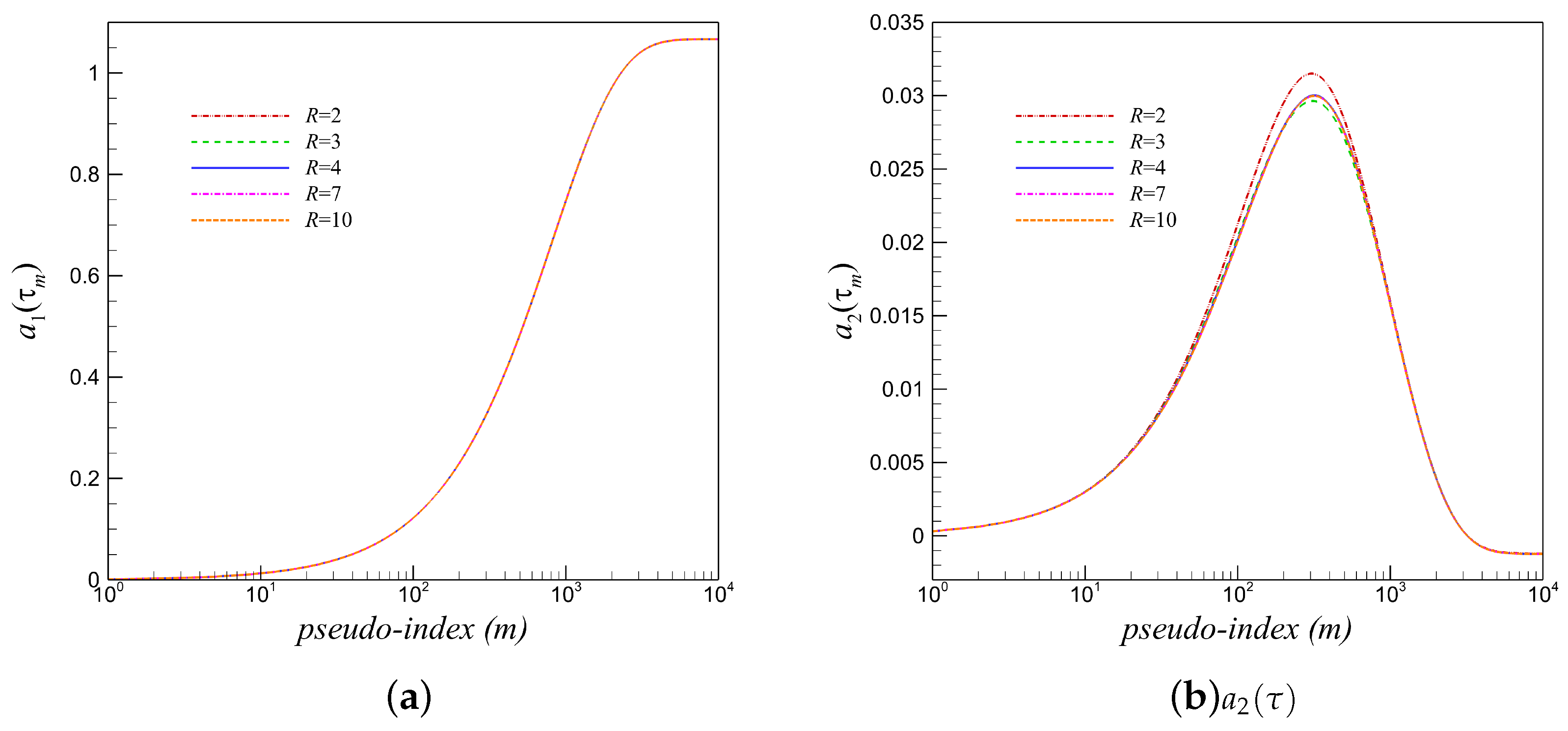
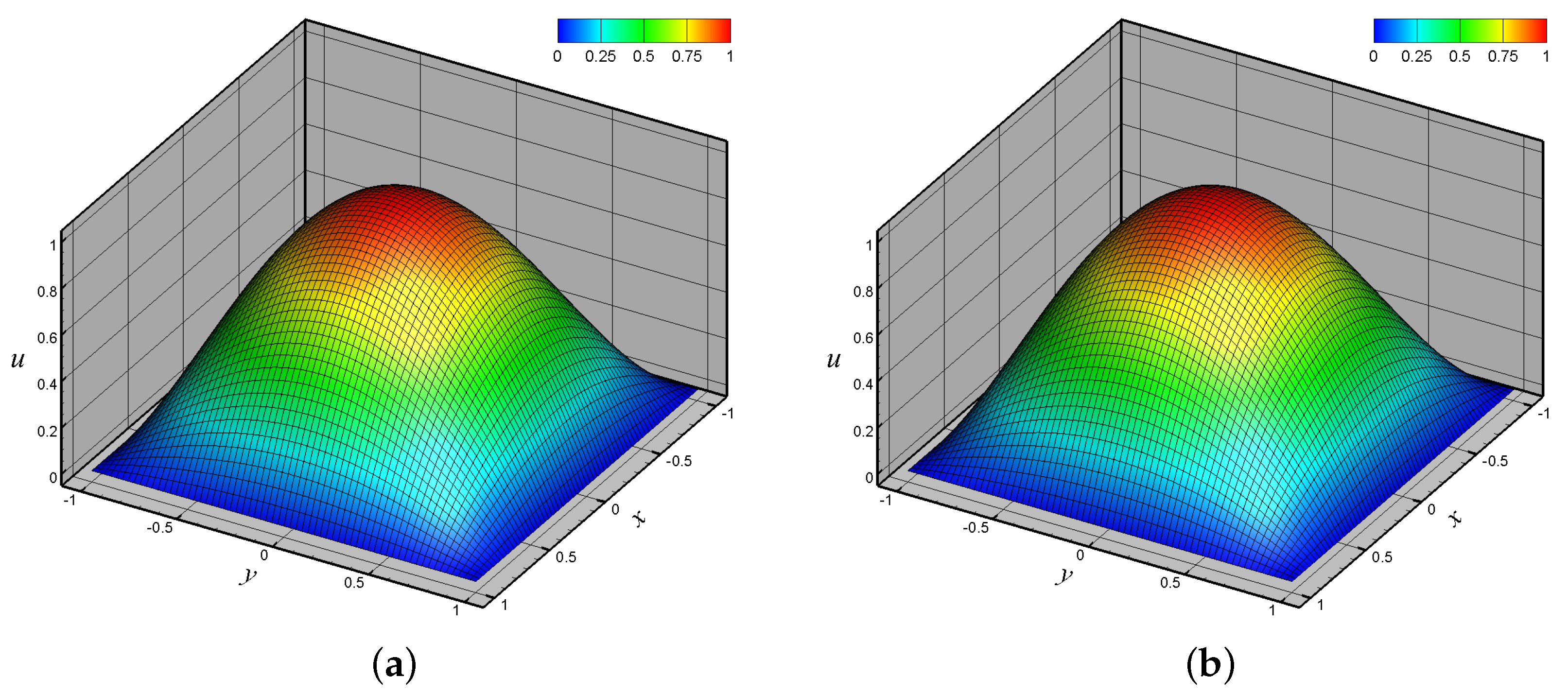
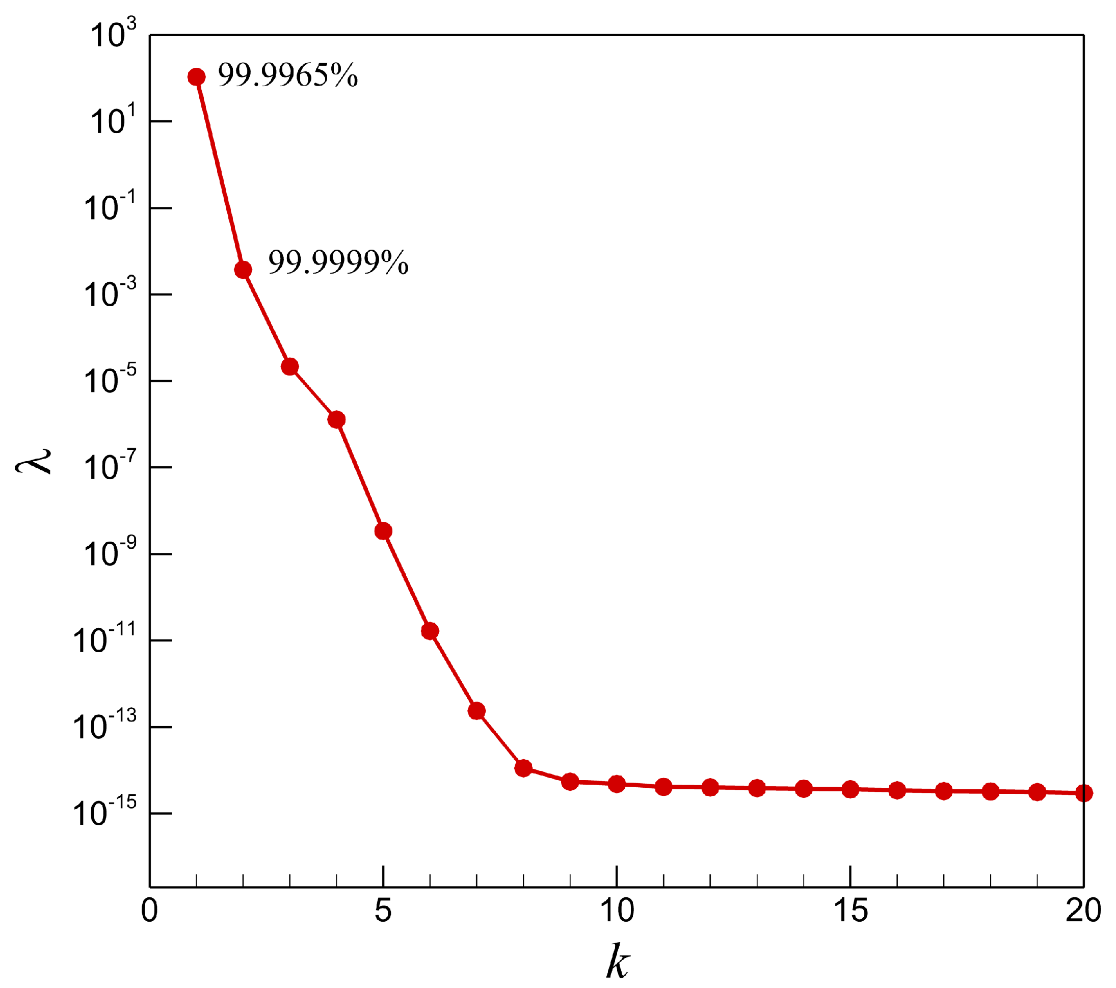
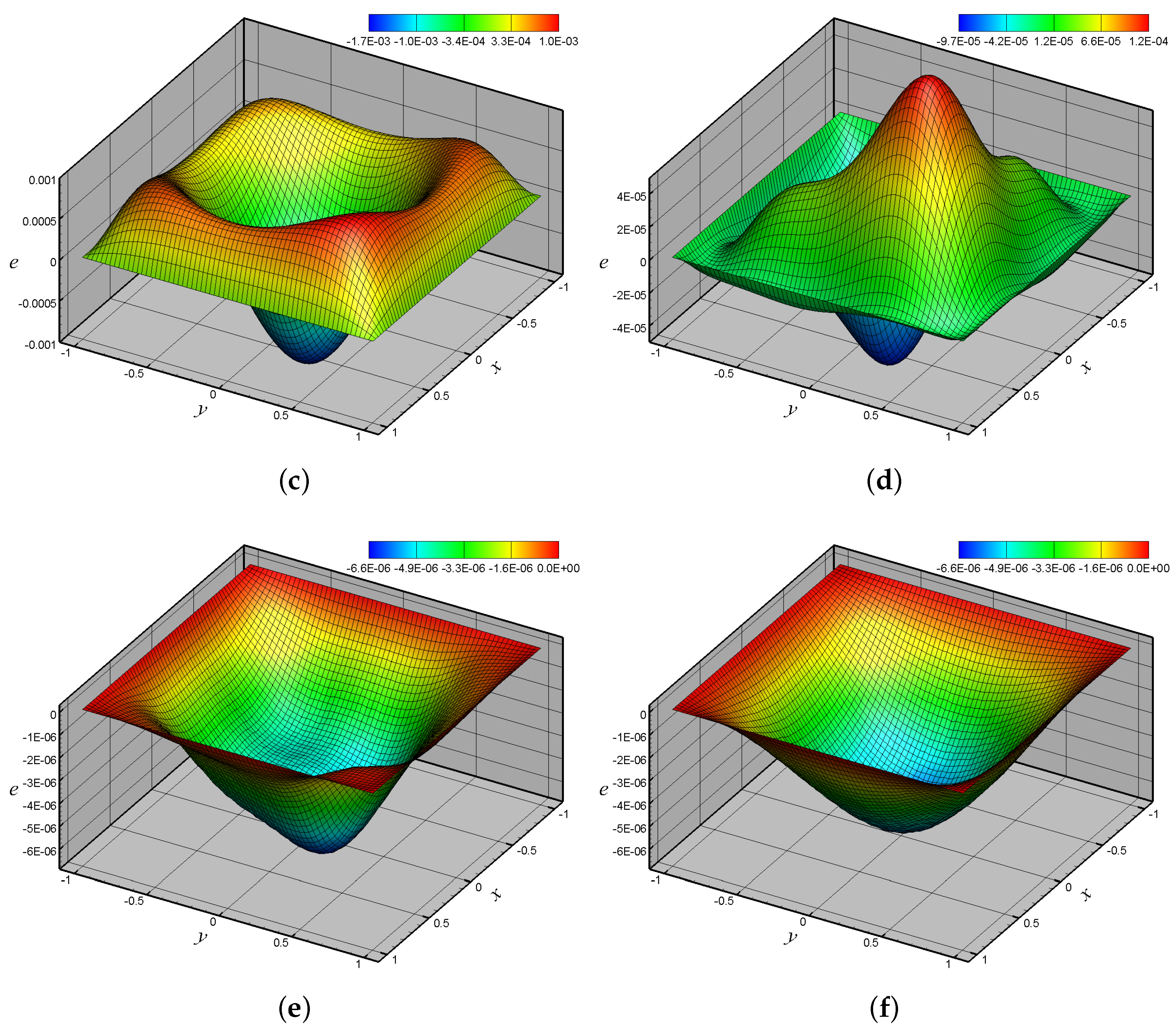
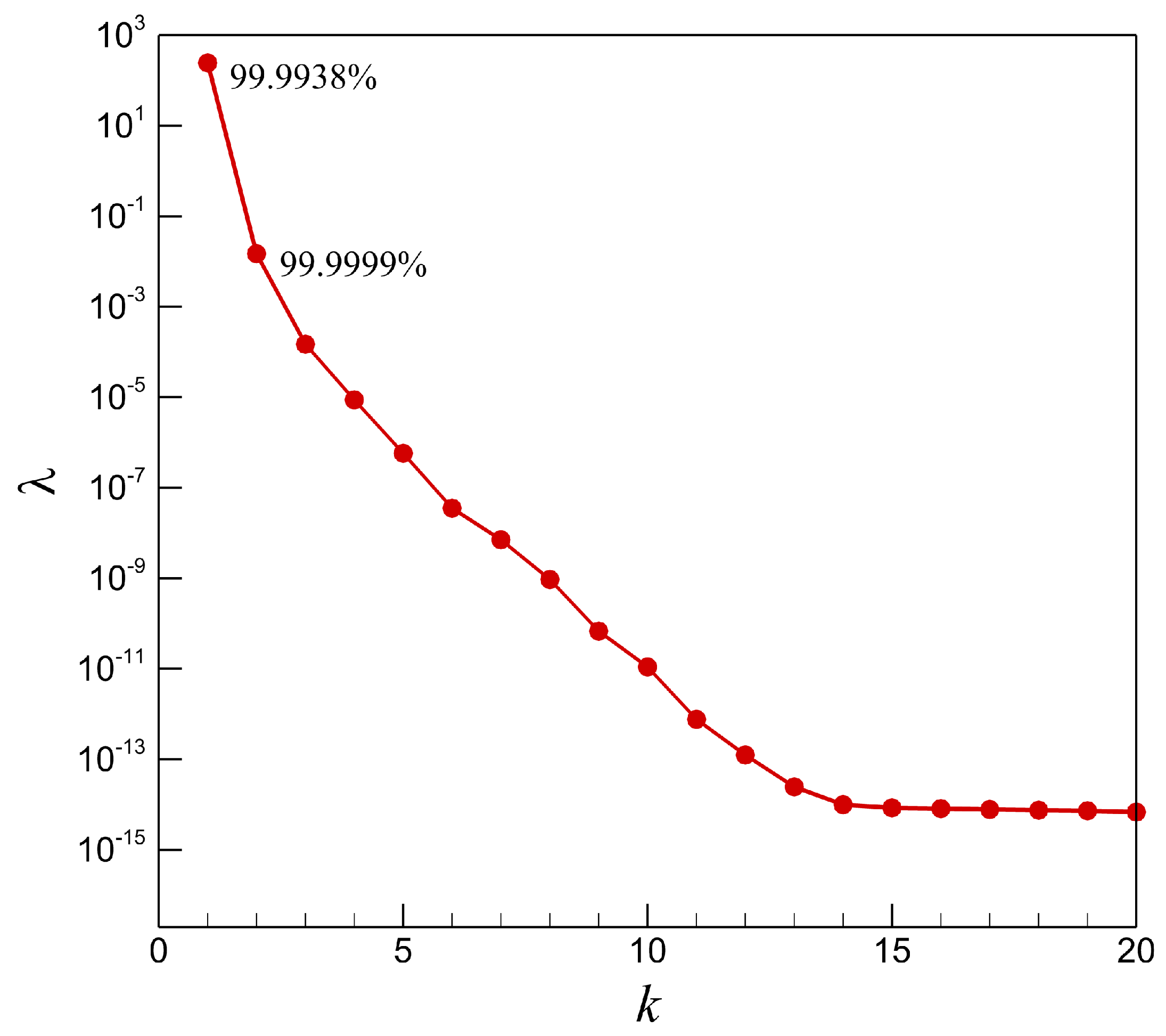
4.1. Reduced Order Modeling Results for a Canonical Elliptic Problem

To validate the Poisson solver in reduced order space, we consider a simple generalized Poisson equation for u field in the Cartesian unit square domain $(x,y)\in {[-1,+1]}^2$ given by

$$\begin{array}{c}\hfill \frac{{\partial }^{2}u}{\partial x^2}+\frac{{\partial }^{2}u}{\partial y^2}=f(x,y),\end{array}$$

(60)

where $f(x,y)=-2(2-x^2-y^2)$ with the Dirichlet boundary condition everywhere on the boundary and the exact solution of the Equation (60) is:

$$\begin{array}{c}\hfill u^{exact}=(x^2-1)(y^2-1).\end{array}$$

(61)

We generate 100 snapshots by solving Equation (60) in full order space by taking ${64}^2$ grid resolution. Then, the POD data correlation matrix is constructed using these 100 snapshots. Figure 2 shows the distribution of eigenvalues of the correlation matrix of u field data with respect to POD index where the figure represents the accumulation of energies in the form of eigenvalue magnitudes. Some corresponding basis functions are plotted in Figure 3. It can be clearly seen that the first mode captures most of the system’s kinetic energy ($99.99\%$). It indicates that this system is very suitable for model order reduction since the energy is concentrated in a very small number of modes. As a result, we can easily exclude other less significant modes to convert it into a low dimensional system. The relaxation histories against the number of iterations of the first two modal coefficients are presented for different POD modes in Figure 4, which means the history of the convergence to steady-state for the modal coefficients. Since we plot in logarithmic scale, it can be easily seen that the change of coefficients in pseudo iterations becomes negligible after 5000 relaxation steps. The number of relaxation iterations can be substantially reduced by choosing a smaller $\Delta \tau$. However, the solution of the Poisson equation in our ROM setting adds a negligibly small computational cost since R is very small. The relaxation history plots also show that the increase of POD modes does not affect the system at all for first modal coefficient rather increasing more modes cause some inaccuracies as observed for the second modal coefficient. This is reasonable since the first mode contains $99.99\%$ of the energy, which is considered a sufficient total kinetic energy for the optimal number of modes in most of the POD studies [95]. In Figure 5, plots (a) and (b) are presented to show a comparative representation between FOM and ROM (for $R=1$). We can say that only one POD mode, i.e., $R=1$ of ROM is generating an almost identical solution to the FOM solution, whereas ROM is taking much less CPU time than the FOM model. By looking at the plots in (c)–(f), it is obvious that errors are slowly increasing with the increase of the number of POD modes. The error for the u field is calculated using Equations (57)–(59). The source of this error can be the over-estimation of true physics in higher modes [95] since it is shown by Iollo et al. [45] that the high frequencies are filtered out when only a few POD modes are retained. For this reason, the higher modes can contain the unwanted frequencies that can be the source of inaccuracies once the optimal mode is found [96]. To further illustrate the quantitative analysis and predictive performance of the ROM model for this particular problem, we tabulated the infinity norm and Euclidean norm for POD modes up to 10 modes in

Table 1. A quantitative analysis and predictive performance of the reduced order modeling (ROM) framework for the canonical elliptic problem solving the Poisson equation.

Poisson Problem (${64}^2$)
ROM Model	$\left|\right|{\mathit{u}}^{\mathit{ROM}}-{\mathit{u}}^{\mathit{Exact}}{\left|\right|}^{\infty }$	$\left|\right|{\mathit{u}}^{\mathit{ROM}}-{\mathit{u}}^{\mathit{Exact}}{\left|\right|}^{\mathbf{2}}$
$R=1$	1.69 × 10${}^{-3}$	6.32 × 10${}^{-4}$
$R=2$	1.20 × 10${}^{-4}$	4.51 × 10${}^{-5}$
$R=3$	3.43 × 10${}^{-5}$	1.21 × 10${}^{-5}$
$R=4$	6.54 × 10${}^{-6}$	3.12 × 10${}^{-6}$
$R=5$	6.26 × 10${}^{-6}$	3.10 × 10${}^{-6}$
$R=7$	6.20 × 10${}^{-6}$	3.10 × 10${}^{-6}$
$R=10$	6.19 × 10${}^{-6}$	3.10 × 10${}^{-6}$

. As we can see, the error magnitudes are bounded and small even if we use a higher number of modes. Even though the error is decreasing with the increment of R, the order of error magnitude is almost constant after $R=4$, which again supports the claim that the higher order modes don’t contribute to the dynamics for this particular problem.

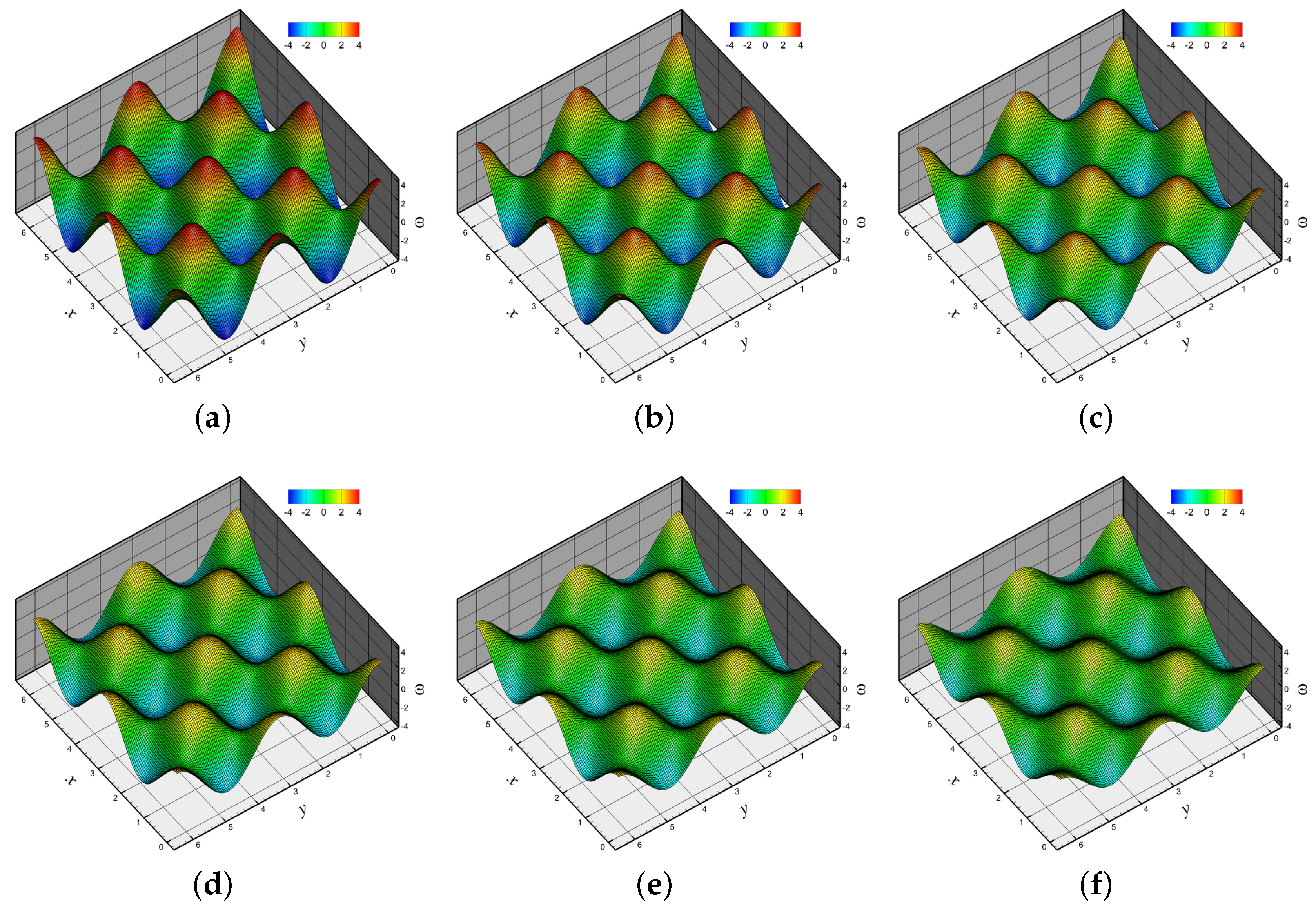
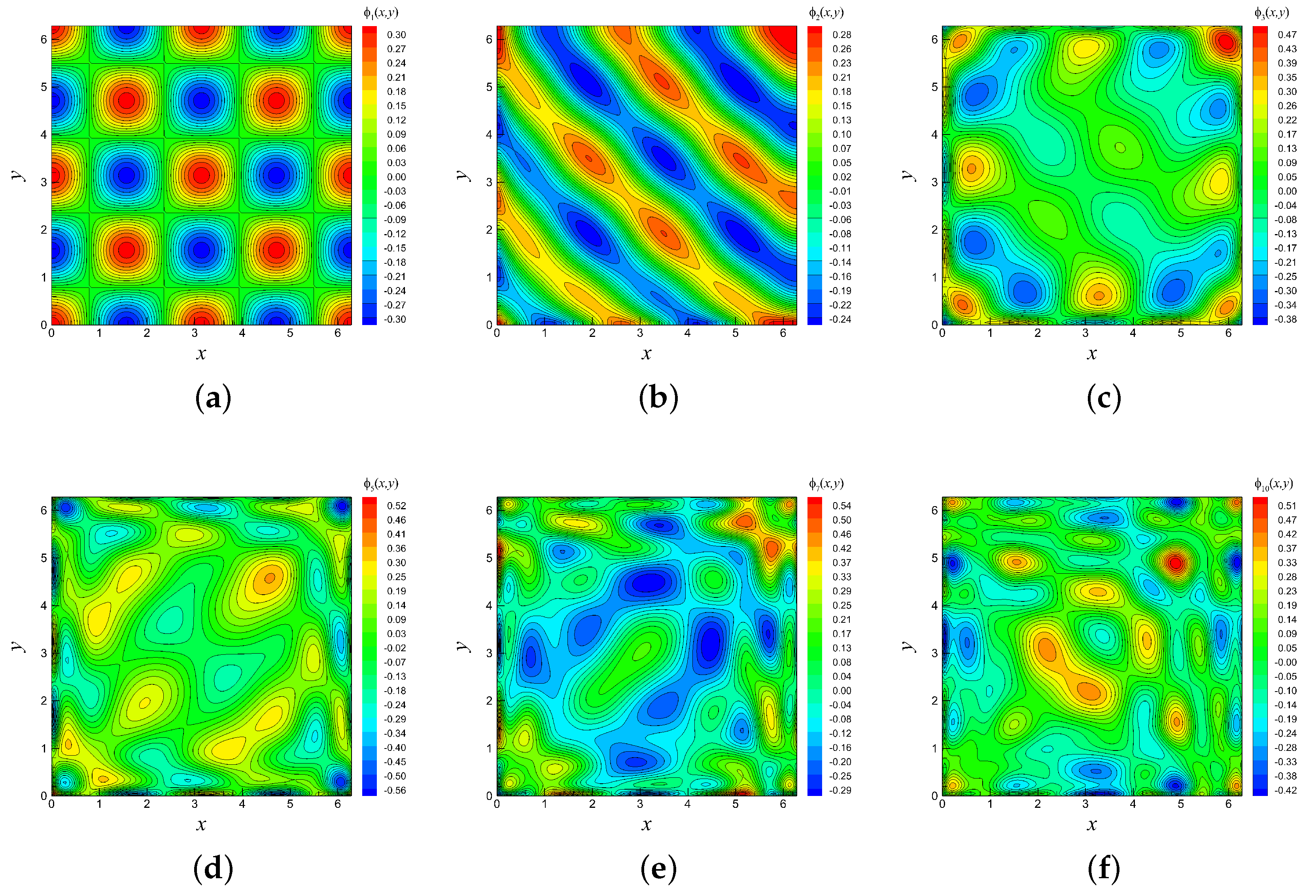
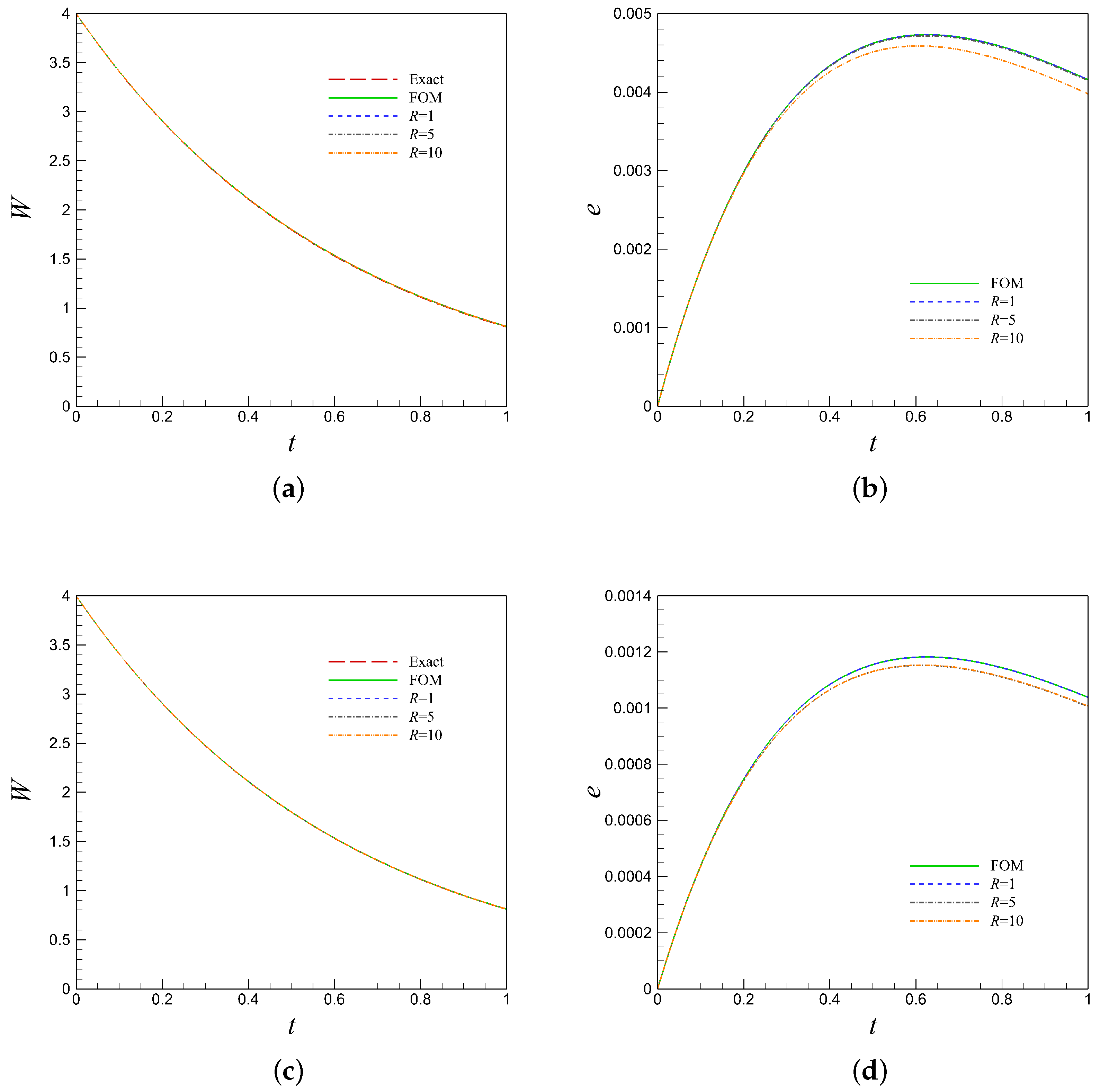
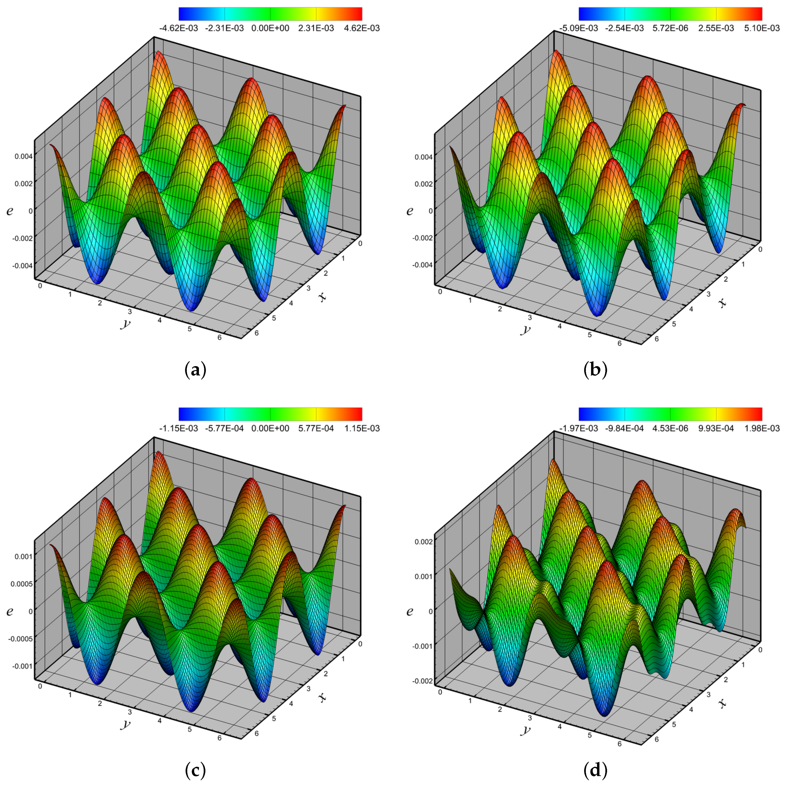
4.2. Hybrid Analytics Results for the Taylor–Green Vortex Decaying Problem

In this section, the HA-ROM model in the vorticity-stream function formulation is analyzed by solving the classical TGV problem in a two-dimensional square domain. TGV problem is a well-defined unsteady flow of a decaying vortex, and is an exact closed form solution of the incompressible Navier–Stokes equations in Cartesian coordinates. As a result, TGV has become one of the most popular numerical test cases for model validation, and has been appeared in a lot of literature [97,98,99,100]. The initial condition of a two-dimensional TGV problem involves the smooth periodic boundary condition and consists of a trigonometric polynomial in all directions. The analytic solution in a uniformly spaced computational domain with an edge length of $2\pi$ is given for a velocity field by

$$\begin{array}{c}{u}^{exact}(x,y,t)=-cos\left(kx\right)sin\left(ky\right)e^{-2k^{2}t/Re},\hfill \end{array}$$

(62)

$$\begin{array}{c}{v}^{exact}(x,y,t)=sin\left(kx\right)cos\left(ky\right)e^{-2k^{2}t/Re},\hfill \end{array}$$

(63)

and, for vorticity and stream function fields,

$$\begin{array}{c}\hfill {\omega }^{exact}(x,y,t)=2kcos\left(kx\right)cos\left(ky\right)e^{-2k^{2}t/Re},\end{array}$$

(64)

$$\begin{array}{c}\hfill {\psi }^{exact}(x,y,t)=\frac{1}{k}cos\left(kx\right)cos\left(ky\right)e^{-2k^{2}t/Re},\end{array}$$

(65)

where k is an integer representing the number of vortices in each direction. In our simulation, we consider $k=2$, Reynolds number, $Re=10$ and grid resolutions of ${64}^2$ or ${128}^2$ with a time step of $1\times {10}^{-3}$ for the TVDRK3 time integration scheme. Figure 6 shows the visual representation of decaying vorticity field with the time evolution for the TGV problem. It can be seen that the dynamics of the problem exhibit only the decaying process. Similar to the eigenvalue magnitude plot in Section 4.1, we plot the eigenvalues of the correlation matrix of stream function data as shown in Figure 7. It is again showing that the first mode contains about $99.99\%$ of energy of the system. Since the nonlinear Jacobian given by Equation (13) becomes nearly zero for this problem, the eigenvalue magnitudes decay rapidly as seen in Figure 7. Contour plots of some POD basis functions are shown in Figure 8 where the smaller structures in the plot are represented by modes corresponding to higher POD indices. It can be noted that the first POD basis function correctly captures the TGV vortex arrays. On the other hand, Aubry et al. [101] showed in their work that a necessary condition for determining the finite number of POD modes needed to derive an accurate finite set of ordinary differential equations is that the truncated system has to inherit the symmetry properties of the original system. In our case, the first POD basis function is well reconstructed, and inherits the symmetric property. We can see in Figure 9 from the error plot of total enstrophy that the effect of higher modes is more pronounced in high resolution simulations for the HA-ROM model. The total enstrophy is calculated using the following expression:

$$\begin{array}{c}\hfill W\left(t\right)=\frac{1}{{\left(2\pi \right)}^2}\int \int {\omega }^2(x,y,t)dxdy.\end{array}$$

(66)

As shown in Figure 9, the total enstrophy versus time plot does not show any significant variations for exact FOM and different POD modes solutions for both ${64}^2$ and ${128}^2$ resolutions. Nonetheless, the close-up error plots show that the $R=10$ solution deviates a little from the FOM, $R=1$ and $R=5$ solutions for ${64}^2$ resolution, yet both $R=5$ and $R=10$ solutions deviate from FOM and $R=1$ solutions for ${128}^2$ resolution. We can conclude from this finding that the higher mode solutions can deviate further if we increase the resolution more. Considering $R=1$ as an ideal case, we develop our HA-ROM model for analysis. In Figure 10, comparison of the FOM and HA-ROM solutions at $t=1$ is presented through errors for vorticity field against $(x,y)$ plots. It can be seen that, for both ${64}^2$ and ${128}^2$ resolutions, the error contour is almost identical. However, the HA-ROM computations take around 136 times (for ${64}^2$ resolution) and 531 times (for ${128}^2$ resolution) less than the FOM computations. To get more quantitative idea, we present the error plot and total CPU time required for both FOM and HA-ROM models (for POD modes up to 10) on ${64}^2$ resolution and ${128}^2$ resolution in

Table 2. A quantitative analysis and predictive performance of the proposed HA-ROM framework for the decaying Taylor-Green vortex (TGV) problem. Note that the error increases with increasing R for this problem because the first mode fully represents the TGV dynamics as shown in Figure 8.

TGV Problem at $\mathit{Re}=10$
Model	CPU Time (${\mathbf{64}}^{\mathbf{2}}$)	$\left|\right|{\mathit{\omega }}_{{\mathbf{64}}^{\mathbf{2}}}^{\mathit{Model}}-{\mathit{\omega }}^{\mathit{Exact}}{\left|\right|}^{\mathbf{2}}$	CPU Time (${\mathbf{128}}^{\mathbf{2}}$)	$\left|\right|{\mathit{\omega }}_{{\mathbf{128}}^{\mathbf{2}}}^{\mathit{Model}}-{\mathit{\omega }}^{\mathit{Exact}}{\left|\right|}^{\mathbf{2}}$
FOM	137.9375 s	2.31 × 10${}^{-3}$	2156.2968 s	5.77 × 10${}^{-4}$
HA-ROM ($R=1$)	1.0156 s	2.42 × 10${}^{-3}$	4.0625 s	8.39 × 10${}^{-4}$
HA-ROM ($R=2$)	1.6250 s	1.05 × 10${}^{-2}$	6.2656 s	5.70 × 10${}^{-3}$
HA-ROM ($R=3$)	2.2187 s	1.20 × 10${}^{-2}$	8.7812 s	5.38 × 10${}^{-3}$
HA-ROM ($R=4$)	3.1406 s	1.65 × 10${}^{-2}$	13.2812 s	6.27 × 10${}^{-3}$
HA-ROM ($R=5$)	5.2187 s	5.08 × 10${}^{-3}$	15.8281 s	6.01 × 10${}^{-3}$
HA-ROM ($R=10$)	12.3583 s	1.64 × 10${}^{-2}$	45.9531 s	4.68 × 10${}^{-3}$

. It can be seen that HA-ROM ($R=1$) solutions, for both resolutions, give errors of the same order magnitude of the FOM solutions, whereas the HA-ROM solutions for higher modes indicate an overestimation of true physics. This can be explained in such a way that the first mode, as shown in Figure 8, represents the TGV dynamics seamlessly. However, we have included higher R values in our analysis in order to show that the error produced by higher POD modes (i.e., overfitting) is bounded. Furthermore, HA-ROM ($R=1$) computations are the fastest among the other mode computations, even though a small amount of accuracy is compromised. Overall, we can say that the HA-ROM ($R=1$) exhibits better predictive characteristics of the FOM solutions in a very short amount of time, i.e., a significant amount of reduction in computational cost can be achieved using the HA-ROM ($R=1$) model for this test case.

5. Conclusions

This study presents a computational framework for accelerating incompressible flow computations. We propose a hybrid analytics paradigm combining physics-based modeling with data-driven modeling. Our physics-based computational model consists of a finite difference approximation of the unsteady two-dimensional Navier–Stokes equation. This model requires solving a Poisson equation at each time step (or sub-stages for multistage Runge-Kutta algorithms), which constitutes a computational stiffness to the problem. Depending on the tolerance set for the Poisson equation, most incompressible flow solvers require $O\left(10\right)$-$O\left({10}^3\right)$ sub-iterations for solving this elliptic sub-problem at each step. Although there are optimal Poisson solvers (e.g., direct solvers such as fast Poisson solvers based on Fast Fourier Transform or its variants, or iterative multigrid solvers), their computational cost still exceeds the computational cost required for the advection–diffusion part of the solver in most computational setups. Therefore, in this study, we have established a numerical approach to reduce the associated computational cost such that proper orthogonal basis functions are generated to be used in solving the elliptic sub-problem in a reduced order space.

The proposed hybrid analytics paradigm addresses the computational stiffness due to computing of such an elliptic sub-problem. We design a reduced-order model for solving the Poisson equation using a projection approach originating from a set of proper orthogonal decomposition basis functions. Unlike the classical iterative solvers for the Poisson equation, we project the source term into a reduced order space (encoder), perform the iterations on that space (ROM), and then transfer the solution back to the full order space (decoder) to continue to the next step. We introduce data transfer procedures (i.e., encoder and decoder formulations) to fulfill these tasks. We emphasize that the computational costs of these mapping procedures are negligibly small.

In order to assess the computational performances of the proposed hybrid analytics method, we consider two numerical experiments. First, we validate the iterative procedure for solving a canonical Poisson equation. Then, we applied the hybrid analytics paradigm for the solution of two-dimensional Navier–Stokes equations considering its vorticity-stream function formulation. The simulations of the decaying Taylor–Green vortex problem are presented to demonstrate the feasibility of our approach. We compare our hybrid approach with the classical full-order finite difference solution as well as with the analytical solution. We perform a quantitative comparison with respect to the number of retained modes in both problems. Significant savings in computational time are found with little compromise to the accuracy of the solutions. Furthermore, we emphasize that our hybrid analytics approach is modular and can be expanded into various formulations for solving a multitude of problems dealing with the incompressibility constraint. The present examples concern very basic flow situations where only a few POD modes dominate the underlying dynamics. In our future studies, we will continue to investigate the validity of the proposed approach for solving three-dimensional flows such as a wake at a rather large Reynolds number. We anticipate that retaining a higher number of POD modes would be necessary to represent more complex flow dynamics.

Although the methodology has been demonstrated for a much simpler problem in comparison to what is expected in the context of Digital Twin, we stress the fact that the field of hybrid analytics research is in its infancy and work is currently ongoing to combine more advanced machine learning algorithms like deep neural network and convolutional neural network with physics-based equations. Such hybrid approaches combining data science methods with physics offer promises in diverse application areas of fluids [102,103,104,105,106,107,108,109], and we will continue to advance this new envisioned field of research.

References

1. Grieves, M. Virtually Perfect: Driving Innovative and Lean Products Through Product Lifecycle Management; Space Coast Press: Cocoa Beach, FL, USA, 2011. [Google Scholar]
2. Colagrossi, A.; Landrini, M. Numerical simulation of interfacial flows by smoothed particle hydrodynamics. J. Comput. Phys. 2003, 191, 448–475. [Google Scholar] [CrossRef]
3. Monaghan, J.J. Simulating free surface flows with SPH. J. Comput. Phys. 1994, 110, 399–406. [Google Scholar] [CrossRef]
4. Magyari, E.; Keller, B. Heat and mass transfer in the boundary layers on an exponentially stretching continuous surface. J. Phys. D Appl. Phys. 1999, 32, 577. [Google Scholar] [CrossRef]
5. Ramamurti, R.; Sandberg, W. Simulation of flow about flapping airfoils using finite element incompressible flow solver. AIAA J. 2001, 39, 253–260. [Google Scholar] [CrossRef]
6. Cebral, J.R.; Yim, P.J.; Löhner, R.; Soto, O.; Choyke, P.L. Blood flow modeling in carotid arteries with computational fluid dynamics and MR imaging. Acad. Radiol. 2002, 9, 1286–1299. [Google Scholar] [CrossRef]
7. Panton, R.L. Incompressible Flow. John Wiley & Sons: New York, NY, USA, 2006. [Google Scholar]
8. Chorin, A.J. A numerical method for solving incompressible viscous flow problems. J. Comput. Phys. 1967, 2, 12–26. [Google Scholar] [CrossRef]
9. Hafez, M.M. Numerical Simulations of Incompressible Flows; World Scientific: Danvers, MA, USA, 2003. [Google Scholar]
10. Quartapelle, L. Numerical Solution of the Incompressible Navier–Stokes Equations; Birkhäuser: Basel, Switzerland, 2013; Volume 113. [Google Scholar]
11. Mateescu, D.; Paıdoussis, M.; Bélanger, F. A time-integration method using artificial compressibility for unsteady viscous flows. J. Sound Vib. 1994, 177, 197–205. [Google Scholar] [CrossRef]
12. Tang, H.; Sotiropoulos, F. Fractional step artificial compressibility schemes for the unsteady incompressible Navier–Stokes equations. Comput. Fluids 2007, 36, 974–986. [Google Scholar] [CrossRef]
13. Kwak, D.; Kiris, C.; Kim, C.S. Computational challenges of viscous incompressible flows. Comput. Fluids 2005, 34, 283–299. [Google Scholar] [CrossRef] [Green Version]
14. Brown, D.L. Accuracy of projection methods for the incompressible Navier–Stokes equations. In Numerical Simulations of Incompressible Flows; World Scientific: Danvers, MA, USA, 2003; pp. 101–107. [Google Scholar]
15. San, O. A novel high-order accurate compact stencil Poisson solver: Application to cavity flows. Int. J. Appl. Mech. 2015, 7, 1550006. [Google Scholar] [CrossRef]
16. Tezduyar, T.; Liou, J.; Ganjoo, D.; Behr, M. Solution techniques for the vorticity–streamfunction formulation of two-dimensional unsteady incompressible flows. Int. J. Numer. Meth. Fluids 1990, 11, 515–539. [Google Scholar] [CrossRef]
17. Arakawa, A. Computational design for long-term numerical integration of the equations of fluid motion: Two-dimensional incompressible flow. Part I. J. Comput. Phys. 1966, 1, 119–143. [Google Scholar] [CrossRef]
18. Wilson, R.V.; Demuren, A.O.; Carpenter, M. Higher-order compact schemes for numerical simulation of incompressible flows. Ins. Comput. Appl. Sci. Eng. 1998, 98-13, 1–41. [Google Scholar]
19. Ferziger, J.H.; Peric, M. Computational Methods for Fluid Dynamics; Springer Science & Business Media: Berlin, Germany, 2012. [Google Scholar]
20. Babaee, H.; Acharya, S. A hybrid staggered/semistaggered finite-difference algorithm for solving time-dependent incompressible Navier–Stokes equations on curvilinear grids. Numer. Heat Trans. Part B Fundam. 2014, 65, 1–26. [Google Scholar] [CrossRef]
21. Dormy, E. An accurate compact treatment of pressure for colocated variables. J. Comput. Phys. 1999, 151, 676–683. [Google Scholar] [CrossRef]
22. Rhie, C.; Chow, W.L. Numerical study of the turbulent flow past an airfoil with trailing edge separation. AIAA J. 1983, 21, 1525–1532. [Google Scholar] [CrossRef]
23. Lin, P. A sequential regularization method for time-dependent incompressible Navier–Stokes equations. SIAM J. Numer. Anal. 1997, 34, 1051–1071. [Google Scholar] [CrossRef]
24. Maday, Y.; Patera, A.T.; Rønquist, E.M. An operator-integration-factor splitting method for time-dependent problems: Application to incompressible fluid flow. J. Sci. Comput. 1990, 5, 263–292. [Google Scholar] [CrossRef]
25. Ye, T.; Mittal, R.; Udaykumar, H.; Shyy, W. An accurate Cartesian grid method for viscous incompressible flows with complex immersed boundaries. J. Comput. Phys. 1999, 156, 209–240. [Google Scholar] [CrossRef]
26. Zang, Y.; Street, R.L.; Koseff, J.R. A non-staggered grid, fractional step method for time-dependent incompressible Navier–Stokes equations in curvilinear coordinates. J. Comput. Phys. 1994, 114, 18–33. [Google Scholar] [CrossRef]
27. Harlow, F.H.; Welch, J.E. Numerical calculation of time-dependent viscous incompressible flow of fluid with free surface. Phys. Fluids 1965, 8, 2182–2189. [Google Scholar] [CrossRef]
28. Van Doormaal, J.; Raithby, G. Enhancements of the SIMPLE method for predicting incompressible fluid flows. Numer. Heat Trans. 1984, 7, 147–163. [Google Scholar]
29. Versteeg, H.; Malalasekera, W. An Introduction to Computational Fluid Dynamics: The Finite Volume Method; John Wiley & Sons: New York, NY, USA, 1995. [Google Scholar]
30. Daescu, D.; Navon, I. A dual-weighted approach to order reduction in 4DVAR data assimilation. Mon. Weather Rev. 2008, 136, 1026–1041. [Google Scholar] [CrossRef]
31. Taira, K.; Brunton, S.L.; Dawson, S.T.; Rowley, C.W.; Colonius, T.; McKeon, B.J.; Schmidt, O.T.; Gordeyev, S.; Theofilis, V.; Ukeiley, L.S. Modal analysis of fluid flows: An overview. AIAA J. 2017, 55, 4013–4041. [Google Scholar] [CrossRef]
32. Cao, Y.; Zhu, J.; Navon, I.M.; Luo, Z. A reduced-order approach to four-dimensional variational data assimilation using proper orthogonal decomposition. Int. J. Numer. Meth. Fluids 2007, 53, 1571–1583. [Google Scholar] [CrossRef]
33. Borggaard, J.; Duggleby, A.; Hay, A.; Iliescu, T.; Wang, Z. Reduced-order modeling of turbulent flows. In Proceedings of the MTNS, Blacksburg, VA, USA, 28 July–1 August 2008. [Google Scholar]
34. San, O.; Borggaard, J. Principal interval decomposition framework for POD reduced-order modeling of convective Boussinesq flows. Int. J. Numer. Meth. Fluids 2015, 78, 37–62. [Google Scholar] [CrossRef]
35. Rowley, C.W.; Dawson, S.T. Model reduction for flow analysis and control. Ann. Rev. Fluid Mech. 2017, 49, 387–417. [Google Scholar] [CrossRef]
36. Moosavi, A.; Stefanescu, R.; Sandu, A. Efficient construction of local parametric reduced order models using machine learning techniques. arXiv, 2015; arXiv:1511.02909. [Google Scholar]
37. Gautier, N.; Aider, J.L.; Duriez, T.; Noack, B.; Segond, M.; Abel, M. Closed-loop separation control using machine learning. J. Fluid Mech. 2015, 770, 442–457. [Google Scholar] [CrossRef] [Green Version]
38. Wan, Z.Y.; Vlachas, P.; Koumoutsakos, P.; Sapsis, T. Data-assisted reduced-order modeling of extreme events in complex dynamical systems. PLoS ONE 2018, 13, e0197704. [Google Scholar] [CrossRef] [PubMed]
39. Mohan, A.T.; Gaitonde, D.V. A deep learning based approach to reduced order modeling for turbulent flow control using LSTM neural networks. arXiv, 2018; arXiv:1804.09269. [Google Scholar]
40. San, O.; Maulik, R. Neural network closures for nonlinear model order reduction. Adv. Comput. Math. 2017. [Google Scholar] [CrossRef]
41. San, O.; Maulik, R. Machine learning closures for model order reduction of thermal fluids. Appl. Math. Model. 2018, 60, 681–710. [Google Scholar] [CrossRef]
42. Puligilla, S.C.; Jayaraman, B. Neural networks as globally optimal multilayer convolution architectures for learning fluid flows. arXiv, 2018; arXiv:1806.08234. [Google Scholar]
43. Wang, Z.; Xiao, D.; Fang, F.; Govindan, R.; Pain, C.; Guo, Y. Model identification of reduced order fluid dynamics systems using deep learning. Int. J. Numer. Meth. Fluids 2018, 86, 255–268. [Google Scholar] [CrossRef]
44. Holmes, P.; Lumley, J.L.; Berkooz, G.; Rowley, C.W. Turbulence, Coherent Structures, Dynamical Systems and Symmetry; Cambridge University Press: New York, NY, USA, 2012. [Google Scholar]
45. Iollo, A.; Lanteri, S.; Désidéri, J.A. Stability properties of POD–Galerkin approximations for the compressible Navier–Stokes equations. Theor. Comput. Fluid Dyn. 2000, 13, 377–396. [Google Scholar] [CrossRef]
46. San, O.; Iliescu, T. A stabilized proper orthogonal decomposition reduced-order model for large scale quasigeostrophic ocean circulation. Adv. Comput. Math. 2015, 41, 1289–1319. [Google Scholar] [CrossRef] [Green Version]
47. Rowley, C.W.; Williams, D.R. Dynamics and control of high-Reynolds-number flow over open cavities. Ann. Rev. Fluid Mech. 2006, 38, 251–276. [Google Scholar] [CrossRef]
48. Bui-Thanh, T.; Willcox, K.; Ghattas, O. Model reduction for large-scale systems with high-dimensional parametric input space. SIAM J. Sci. Comput. 2008, 30, 3270–3288. [Google Scholar] [CrossRef]
49. Ito, K.; Ravindran, S. A reduced-order method for simulation and control of fluid flows. J. Comput. Phys. 1998, 143, 403–425. [Google Scholar] [CrossRef]
50. Narasimha, R. Kosambi and proper orthogonal decomposition. Resonance 2011, 16, 574–581. [Google Scholar] [CrossRef]
51. Jin, M.; Liu, W.; Chen, Q. Accelerating fast fluid dynamics with a coarse-grid projection scheme. HVAC R Res. 2014, 20, 932–943. [Google Scholar] [CrossRef]
52. Lentine, M.; Zheng, W.; Fedkiw, R. A novel algorithm for incompressible flow using only a coarse grid projection. ACM Trans. Graph. 2010, 29, 114. [Google Scholar] [CrossRef]
53. San, O.; Staples, A.E. A coarse-grid projection method for accelerating incompressible flow computations. J. Comput. Phys. 2013, 233, 480–508. [Google Scholar] [CrossRef]
54. San, O.; Staples, A.E. An efficient coarse grid projection method for quasigeostrophic models of large-scale ocean circulation. Int. J. Multiscale Comput. Eng. 2013, 11, 463–495. [Google Scholar] [CrossRef]
55. Kashefi, A.; Staples, A.E. A finite-element coarse-grid projection method for incompressible flow simulations. Adv. Comput. Math. 2017. [Google Scholar] [CrossRef]
56. Wesseling, P. An Introduction to Multigrid Methods; John Wiley & Sons: Hoboken, NJ, USA, 1995. [Google Scholar]
57. Filelis-Papadopoulos, C.K.; Gravvanis, G.A.; Lipitakis, E.A. On the numerical modeling of convection-diffusion problems by finite element multigrid preconditioning methods. Adv. Eng. Softw. 2014, 68, 56–69. [Google Scholar] [CrossRef]
58. Reusken, A. Fourier analysis of a robust multigrid method for convection-diffusion equations. Numer. Math. 1995, 71, 365–397. [Google Scholar] [CrossRef] [Green Version]
59. Zhang, J. Fast and high accuracy multigrid solution of the three dimensional Poisson equation. J. Comput. Phys. 1998, 143, 449–461. [Google Scholar] [CrossRef]
60. Drikakis, D.; Iliev, O.; Vassileva, D. Acceleration of multigrid flow computations through dynamic adaptation of the smoothing procedure. J. Comput. Phys. 2000, 165, 566–591. [Google Scholar] [CrossRef]
61. Moin, P. Fundamentals of Engineering Numerical Analysis; Cambridge University Press: New York, NY, USA, 2010. [Google Scholar]
62. Jacobsen, D.; Thibault, J.; Senocak, I. An MPI-CUDA implementation for massively parallel incompressible flow computations on multi-GPU clusters. In Proceedings of the 48th AIAA Aerospace Sciences Meeting Including the New Horizons Forum and Aerospace Exposition, Orlando, FL, USA, 4–7 January 2010; p. 522. [Google Scholar]
63. Thibault, J.C.; Senocak, I. Accelerating incompressible flow computations with a Pthreads-CUDA implementation on small-footprint multi-GPU platforms. J. Supercomput. 2012, 59, 693–719. [Google Scholar] [CrossRef]
64. Jobelin, M.; Lapuerta, C.; Latché, J.C.; Angot, P.; Piar, B. A finite element penalty–projection method for incompressible flows. J. Comput. Phys 2006, 217, 502–518. [Google Scholar] [CrossRef]
65. Korczak, K.Z.; Patera, A.T. An isoparametric spectral element method for solution of the Navier–Stokes equations in complex geometry. J. Comput. Phys. 1986, 62, 361–382. [Google Scholar] [CrossRef]
66. Guermond, J.L.; Minev, P.; Shen, J. Error analysis of pressure-correction schemes for the time-dependent Stokes equations with open boundary conditions. SIAM J. Numer. Anal. 2005, 43, 239–258. [Google Scholar] [CrossRef]
67. Chorin, A.J. Numerical solution of the Navier–Stokes equations. Math. Comput. 1968, 22, 745–762. [Google Scholar] [CrossRef]
68. Temam, R. Approximation of the solution of the Navier–Stokes equations by the fractional step method. Arch. Ration. Mech. Anal. 1969, 32, 135–153. [Google Scholar] [CrossRef]
69. Kim, J.; Moin, P. Application of a fractional-step method to incompressible Navier–Stokes equations. J. Comput. Phys. 1985, 59, 308–323. [Google Scholar] [CrossRef]
70. Tyliszczak, A. A high-order compact difference algorithm for half-staggered grids for laminar and turbulent incompressible flows. J. Comput. Phys. 2014, 276, 438–467. [Google Scholar] [CrossRef]
71. San, O.; Staples, A.E. High-order methods for decaying two-dimensional homogeneous isotropic turbulence. Comput. Fluids 2012, 63, 105–127. [Google Scholar] [CrossRef] [Green Version]
72. Gottlieb, S.; Shu, C.W. Total variation diminishing Runge-Kutta schemes. Math. Comput. Am. Math. Soc. 1998, 67, 73–85. [Google Scholar] [CrossRef] [Green Version]
73. Shu, C.W.; Osher, S. Efficient implementation of essentially non-oscillatory shock-capturing schemes, II. In Upwind and High-Resolution Schemes; Springer: Heidelberg, Germany, 1989; pp. 328–374. [Google Scholar]
74. Gottlieb, S.; Shu, C.W.; Tadmor, E. Strong stability-preserving high-order time discretization methods. SIAM Rev. 2001, 43, 89–112. [Google Scholar] [CrossRef]
75. Zhang, K.K.; Shotorban, B.; Minkowycz, W.; Mashayek, F. A compact finite difference method on staggered grid for Navier–Stokes flows. Int. J. Numer. Meth. Fluids 2006, 52, 867–881. [Google Scholar] [CrossRef]
76. Sirovich, L. Turbulence and the dynamics of coherent structures. I. Coherent structures. Q. Appl. Math. 1987, 45, 561–571. [Google Scholar] [CrossRef] [Green Version]
77. Leblond, C.; Allery, C.; Inard, C. An optimal projection method for the reduced-order modeling of incompressible flows. Comput. Meth. Appl. Mech. Eng. 2011, 200, 2507–2527. [Google Scholar] [CrossRef]
78. Ravindran, S.S. A reduced-order approach for optimal control of fluids using proper orthogonal decomposition. Int. J. Numer. Meth. Fluids 2000, 34, 425–448. [Google Scholar] [CrossRef]
79. Rapún, M.L.; Vega, J.M. Reduced order models based on local POD plus Galerkin projection. J. Comput. Phys. 2010, 229, 3046–3063. [Google Scholar] [CrossRef] [Green Version]
80. Sirisup, S.; Karniadakis, G. Stability and accuracy of periodic flow solutions obtained by a POD-penalty method. Phys. D Nonlinear Phenom. 2005, 202, 218–237. [Google Scholar] [CrossRef]
81. Amsallem, D.; Farhat, C. Stabilization of projection-based reduced-order models. Int. J. Numer. Meth. Eng. 2012, 91, 358–377. [Google Scholar] [CrossRef]
82. Bergmann, M.; Bruneau, C.H.; Iollo, A. Enablers for robust POD models. J. Comput. Phys. 2009, 228, 516–538. [Google Scholar] [CrossRef] [Green Version]
83. Alonso, D.; Velazquez, A.; Vega, J. A method to generate computationally efficient reduced order models. Comput. Meth. Appl. Mech. Eng. 2009, 198, 2683–2691. [Google Scholar] [CrossRef] [Green Version]
84. San, O.; Iliescu, T. Proper orthogonal decomposition closure models for fluid flows: Burgers equation. Int. J. Numer. Anal. Model. Ser. B 2014, 5, 217–237. [Google Scholar]
85. Amsallem, D.; Farhat, C. On the stability of reduced-order linearized computational fluid dynamics models based on POD and Galerkin projection: Descriptor vs. non-descriptor forms. In Reduced Order Methods for Modeling and Computational Reduction; Springer: New York, NY, USA, 2014; pp. 215–233. [Google Scholar]
86. Xie, X.; Mohebujjaman, M.; Rebholz, L.; Iliescu, T. Data-driven filtered reduced order modeling of fluid flows. SIAM J. Sci. Comput. 2018, 40, 834–857. [Google Scholar] [CrossRef]
87. Wang, Z.; Akhtar, I.; Borggaard, J.; Iliescu, T. Proper orthogonal decomposition closure models for turbulent flows: a numerical comparison. Comput. Meth. Appl. Mech. Eng. 2012, 237, 10–26. [Google Scholar] [CrossRef]
88. Kalb, V.L.; Deane, A.E. An intrinsic stabilization scheme for proper orthogonal decomposition based low-dimensional models. Phys. Fluids 2007, 19, 054106. [Google Scholar] [CrossRef]
89. Hoffman, J.D. Numerical Methods for Engineers and Scientists; Marcel Dekker, Inc.: New York, NY, USA, 2001. [Google Scholar]
90. Drikakis, D.; Fureby, C.; Grinstein, F.F.; Youngs, D. Simulation of transition and turbulence decay in the Taylor–Green vortex. J. Turbul. 2007, 8, N20. [Google Scholar] [CrossRef]
91. Moser, R.D.; Kim, J.; Mansour, N.N. Direct numerical simulation of turbulent channel flow up to Re τ = 590. Phys. Fluids 1999, 11, 943–945. [Google Scholar] [CrossRef]
92. Rana, Z.A.; Thornber, B.; Drikakis, D. Transverse jet injection into a supersonic turbulent cross-flow. Phys. Fluids 2011, 23, 046103. [Google Scholar] [CrossRef]
93. Drikakis, D. Advances in turbulent flow computations using high-resolution methods. Prog. Aeros. Sci. 2003, 39, 405–424. [Google Scholar] [CrossRef] [Green Version]
94. Bachant, P.; Wosnik, M. Characterising the near-wake of a cross-flow turbine. J. Turbul. 2015, 16, 392–410. [Google Scholar] [CrossRef]
95. Cordier, L.; Majd, E.; Abou, B.; Favier, J. Calibration of POD reduced-order models using Tikhonov regularization. Int. J. Numer. Meth. Fluids 2010, 63, 269–296. [Google Scholar] [CrossRef] [Green Version]
96. Gloerfelt, X. Compressible POD/Galerkin reduced-order model of self-sustained oscillations in a cavity. In Proceedings of the 12th AIAA/CEAS Aeroacoustics Conference (27th AIAA Aeroacoustics Conference), Cambridge, MA, USA, 8–10 May 2006; p. 2432. [Google Scholar]
97. Shu, C.W.; Don, W.S.; Gottlieb, D.; Schilling, O.; Jameson, L. Numerical convergence study of nearly incompressible, inviscid Taylor–Green vortex flow. J. Sci. Comput. 2005, 24, 1–27. [Google Scholar] [CrossRef]
98. Cox, C.; Liang, C.; Plesniak, M.W. A flux reconstruction solver for unsteady incompressible viscous flow using artificial compressibility with implicit dual time stepping. In Proceedings of the 54th AIAA Aerospace Sciences Meeting, San Diego, CA, USA, 4–8 January 2016; p. 1827. [Google Scholar]
99. Morf, R.H.; Orszag, S.A.; Frisch, U. Spontaneous singularity in three-dimensional inviscid, incompressible flow. Phys. Rev. Lett. 1980, 44, 572. [Google Scholar] [CrossRef]
100. Orszag, S.A. Numerical simulation of incompressible flows within simple boundaries: Accuracy. J. Fluid Mech. 1971, 49, 75–112. [Google Scholar] [CrossRef]
101. Aubry, N.; Lian, W.Y.; Titi, E.S. Preserving symmetries in the proper orthogonal decomposition. SIAM J. Sci. Comput. 1993, 14, 483–505. [Google Scholar] [CrossRef]
102. Milano, M.; Koumoutsakos, P. Neural network modeling for near wall turbulent flow. J. Comput. Phys. 2002, 182, 1–26. [Google Scholar] [CrossRef]
103. Weymouth, G.D.; Yue, D.K. Physics-based learning models for ship hydrodynamics. J. Ship Res. 2013, 57, 1–12. [Google Scholar] [CrossRef]
104. Bai, Z.; Brunton, S.L.; Brunton, B.W.; Kutz, J.N.; Kaiser, E.; Spohn, A.; Noack, B.R. Data-driven methods in fluid dynamics: Sparse classification from experimental data. In Whither Turbulence and Big Data in the 21st Century? Springer: New York, NY, USA, 2017; pp. 323–342. [Google Scholar]
105. Wang, J.X.; Wu, J.L.; Xiao, H. Physics-informed machine learning approach for reconstructing Reynolds stress modeling discrepancies based on DNS data. Phys. Rev. Fluids 2017, 2, 034603. [Google Scholar] [CrossRef]
106. Beck, A.D.; Flad, D.G.; Munz, C.D. Neural networks for data-based turbulence models. arXiv, 2018; arXiv:1806.04482. [Google Scholar]
107. Berger, J.; Mazuroski, W.; Oliveira, R.C.; Mendes, N. Intelligent co-simulation: Neural network vs. proper orthogonal decomposition applied to a 2D diffusive problem. J. Build. Perform. Simul. 2018. [Google Scholar] [CrossRef]
108. San, O.; Maulik, R. Extreme learning machine for reduced order modeling of turbulent geophysical flows. Phys. Rev. E 2018, 97, 042322. [Google Scholar] [CrossRef] [PubMed] [Green Version]
109. Pathak, J.; Wikner, A.; Fussell, R.; Chandra, S.; Hunt, B.R.; Girvan, M.; Ott, E. Hybrid forecasting of chaotic processes: Using machine learning in conjunction with a knowledge-based model. Chaos 2018, 28, 041101. [Google Scholar] [CrossRef] [Green Version]
Figure 1. The proposed hybrid analytics paradigm.
Fluids 03 00050 g001
Figure 2. Eigenvalues of the correlation matrix of u field data.
Fluids 03 00050 g002
Figure 3. Contour plots of some illustrative proper orthogonal decomposition (POD) basis functions generated by the method of snapshots for the Poisson equation: (a) ϕ 1 ( x , y ) ; (b) ϕ 2 ( x , y ) ; (c) ϕ 3 ( x , y ) ; (d) ϕ 5 ( x , y ) ; (e) ϕ 7 ( x , y ) ; (f) ϕ 10 ( x , y ) .
Fluids 03 00050 g003
Figure 4. Relaxation histories for the first two modal coefficients. (a) a 1 ( τ ) ; (b) a 2 ( τ ) .
Fluids 03 00050 g004
Figure 5. Comparison of the full order model (FOM) and reduced order modeling (ROM) solutions on a resolution of 64 2 grid. (a) FOM solution (CPU time: 1.9062 s); (b) ROM ( R = 1 ) solution (CPU time: 0.001565 s); (c) error (i.e., e = u R = 1 R O M u E x a c t ); (d) error (i.e., e = u R = 2 R O M u E x a c t ); (e) error (i.e., e = u R = 4 R O M u E x a c t ); (f) error (i.e., e = u R = 10 R O M u E x a c t ).
Fluids 03 00050 g005aFluids 03 00050 g005b
Figure 6. Evolution of the vorticity field for the Taylor-Green vortex (TGV) decaying problem for κ = 2 . (a) t = 0 ; (b) t = 2 ; (c) t = 4 ; (d) t = 6 ; (e) t = 8 ; (f) t = 10 .
Fluids 03 00050 g006
Figure 7. Eigenvalues of the correlation matrix of stream function data.
Fluids 03 00050 g007
Figure 8. Contour plots of some illustrative POD basis functions generated by the method of snapshots: (a) ϕ 1 ( x , y ) ; (b) ϕ 2 ( x , y ) ; (c) ϕ 3 ( x , y ) ; (d) ϕ 5 ( x , y ) ; (e) ϕ 7 ( x , y ) ; (f) ϕ 10 ( x , y ) .
Fluids 03 00050 g008
Figure 9. Evolution of the domain integrated total enstrophy for the decaying TGV problem at R e = 10 . (a) total enstrophy ( 64 2 ); (b) error (i.e., e = W 64 2 M o d e l W E x a c t ); (c) total enstrophy ( 128 2 ); (d) error (i.e., e = W 128 2 M o d e l W E x a c t ).
Fluids 03 00050 g009
Figure 10. Comparison of the FOM and HA-ROM (i.e., R = 1 ) solutions at t = 1 for the TGV problem at R e = 10 . Required CPU times for the FOM simulations are 137.9375 s ( 64 2 ) and 2156.2968 s ( 128 2 ). However, the HA-ROM computations require only 1.0156 s ( 64 2 ) and 4.0625 s ( 128 2 ) CPU time; (a) error (i.e., e = ω 64 2 F O M ω E x a c t ); (b) error (i.e., e = ω 64 2 H A R O M ω E x a c t ); (c) error (i.e., e = ω 128 2 F O M ω E x a c t ); (d) error (i.e., e = ω 128 2 H A R O M ω E x a c t ).
Fluids 03 00050 g010