Flow Structure and Force Generation on Flapping Wings at Low Reynolds Numbers Relevant to the Flight of Tiny Insects

Abstract

In contrast to larger species, little is known about the flight of the smallest flying insects, such as thrips and fairyflies. These tiny animals range from 300 to 1000 microns in length and fly at Reynolds numbers ranging from about 4 to 60. Previous work with numerical and physical models have shown that the aerodynamics of these diminutive insects is significantly different from that of larger animals, but most of these studies have relied on two-dimensional approximations. There can, however, be significant differences between two- and three-dimensional flows, as has been found for larger insects. To better understand the flight of the smallest insects, we have performed a systematic study of the forces and flow structures around a three-dimensional revolving elliptical wing. We used both a dynamically scaled physical model and a three-dimensional computational model at Reynolds numbers ranging from 1 to 130 and angles of attacks ranging from 0° to 90°. The results of the physical and computational models were in good agreement and showed that dimensionless drag, aerodynamic efficiency, and spanwise flow all decrease with decreasing Reynolds number. In addition, both the leading and trailing edge vortices remain attached to the wing over the scales relevant to the smallest flying insects. Overall, these observations suggest that there are drastic differences in the aerodynamics of flight at the scale of the smallest flying animals.

1. Introduction

The smallest flying insects are on the order of 1 mm or less in body length, and some species of fairyflies are less than 250 µm long [1]. These insects are of significant agricultural, ecological, and economic importance. Thrips are a common agricultural pest [2,3], and parasitoid wasps have the potential for use in biological control of agricultural pests [4,5]. For example, a recent study demonstrated that the successful control of thrips using a small predatory insect resulted in an economic benefit of nearly $60 million in California [6]. These tiny insects can also transmit pollen [7,8] and serve as biological vectors for plant pathogens through mechanical transmission [9,10].

Typically, the smallest insects flap their wings at frequencies greater than 200 Hz [11,12] with some insects such as mosquitos reaching frequencies above 800 Hz [13]. At this scale and wingbeat frequency, viscous forces are significant, and the relevant Reynolds numbers (Re) are on the order of 4 to 60. Previous work has shown that the wing kinematics and aerodynamics of the smallest insects are significantly different from those of their larger counterparts [11,12,14,15,16,17,18,19,20,21,22,23,24,25,26]. Whereas one might assume that such small insects would be dependent upon wind currents for locomotion (and this may be true for long distance travel), they are nevertheless capable of controlled flight over short distances [7]. Understanding the aerodynamics of flapping flight at this small scale may lead to improved dispersal strategies for biological control. Additionally, further insight into the aerodynamic limits of flight in tiny insects may be beneficial to engineers developing biologically-inspired micro-aerial vehicles [27].

Computational fluid dynamics provides a convenient framework for comparing the flight of small and large insects. For example, the forces and flow structures around flapping wings can be compared over a range of Re simply by changing the dynamic viscosity while holding all other parameters constant. In a two-dimensional numerical study, Wang [25] showed that when the Re was lowered from 157 to 15.7, the lift coefficients decreased by more than 50%. Similarly, Wu and Sun showed that lift coefficients decreased and drag coefficients increased when the Re decreased from 1800 to 20 in three-dimensional simulations [28]. Miller and Peskin [20] found that at Re < 32, the flow patterns around a wing are different from those with Re > 64 in two-dimensional simulations. They also showed that the force required to pull two wings apart during a clap and fling motion [12] is greater at lower Re [21], however, these forces are somewhat reduced by wing flexibility [22].

Most studies relevant to the flight of tiny insects have been performed in two dimensions [11,18,20,21,22,26,29,30,31]. While valuable information can be obtained from two-dimensional studies, previous research shows that critical differences exist between two- and three- dimensional studies for larger insects. In general, two-dimensional studies fail to capture three-dimensional effects such as spanwise flow, and there can be differences in the separation of the leading edge vortex [31]. Many of these differences relate to the fact that insect wings revolve around their root—like a helicopter blade—and, thus, flows are under the influence of three-dimensional phenomena such as Coriolis forces [32].

A few studies have modeled tiny insect flight in three dimensions. Sun and Yu [23] investigated the flight of a tiny insect at Re = 15. Kolomenskiy et al. [17] modeled three-dimensional effects during the clap and fling, but did not consider Re below 128. Based on a computational model, Liu and Aono [33] found that a thrips (Re = 10) did not produce as much force as a fruit fly (Re = 134), but they did not explore the range of Re between these two cases.

In this study, we used both a dynamically scaled physical model and a three-dimensional computational model to investigate the effect of changing Re from 1 to 130 on the generation of aerodynamic forces and the flow structures of a three-dimensional elliptical wing. The specific objective was to characterize the flows and forces generated by the steady motion of a revolving wing over a range of Re and angles of attack relevant to the hovering flight of the smallest insects [34,35,36,37]. As a result, some of the features observed in the actual flapping kinematics such as variation in rotational phase, motion perpendicular to the stroke plane, and variations in angle of attack during a stroke [38] were not considered in this study. However, using the computational model, we could explore three-dimensional effects, such as spanwise flow. Our results show that as Re decreases, drag increases significantly, aerodynamic efficiency decreases, spanwise flow decreases, and the leading edge vortex (LEV) and trailing edge vortex (TEV) do not separate from the wing.

2. Methods

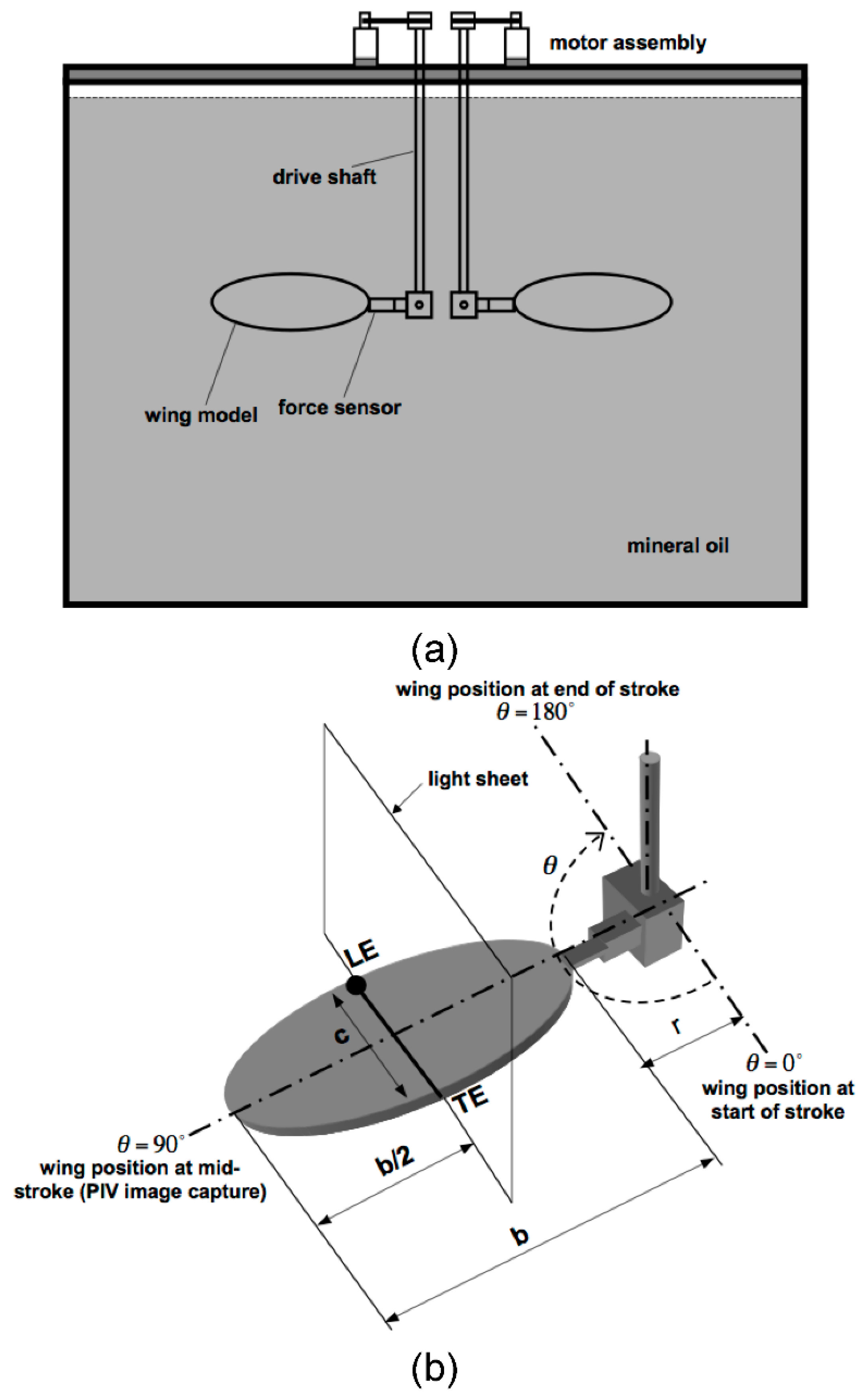
2.1. Dynamically Scaled Model Wing

Force and flow field measurements were obtained using a dynamically scaled physical model (Figure 1), which has been described in detail elsewhere [39,40,41]. The experimental system consisted of a wing attached to a coaxial arm, immersed in a 1 m × 1 m × 2 m tank filled with mineral oil. Computer-driven servo-motors controlled the orientation and movement of the wing, while force sensors recorded the lift and drag. Although the experimental system consists of two wings, only a single arm and wing were used in this study. We constructed a wing from a 2.0 mm thick clear acrylic sheet with an elliptical planform with a maximum chord length, c, of 8.25 cm and span, b, of 16.5 cm. The force sensor connected the base of the wing to the end of the arm, resulting in a wingtip radius, R, of 20.1 cm.

The Reynolds number was calculated as

$$Re=\frac{\overline{\omega }Rc\rho }{\mu },$$

(1)

where $\overline{\omega }$ is the angular velocity of the wing tip during the steady portion of the revolution, $\rho$ is the fluid density, and $\mu$ is the dynamic viscosity of the fluid. Aerodynamics forces were measured for Re = 130, and flow was visualized using DPIV for Re ranging from 1 to 100. The tank was filled with mineral oil (ρ = 830 kg·m⁻³; µ = 996 × 10⁻⁴ kg·m⁻¹·s⁻¹).

The lift and drag coefficients were calculated according to [40] as

$$C_F=\frac{2F}{\rho {\overline{\omega }}^2{R}^3\overline{c}{\widehat{r}}_2^2\left(S\right)},$$

(2)

where F is a specific force component (lift, drag, total), $\overline{c}$ is the mean chord length, R is the wing length, and ${\widehat{r}}_2^2$(S) is the non-dimensional second moment of wing area.

2.2. Kinematics

The drive system of the experimental system provided the model wing with a 2-degree of freedom motion, which included pitching about the spanwise axis (that is, changes in angle of attack) and rotation about the axis of the arm (that is, sweeping within the stroke plane). The kinematic pattern used in this study consisted of a single wing revolving once through an 180° arc in a horizontal stroke plane with constant angular velocity at a fixed angle of attack (Figure 1b), with the angle of attack varied from −9° to 99°. The angular velocity of wing revolution was varied trapezoidally, such that the first 10% of each stroke consisted of constant acceleration, followed by constant velocity (80%) and then constant deceleration (10%). Note that this is a simplification of the actual motion of low Re insects as any changes in angle of attack or deviations from a horizontal stroke plane are neglected. In the experimental cases, the system was kept at rest for no less than 3 minutes to ensure the fluid had come to rest.

2.3. Flow Visualization

We used digital particle image velocimetry (DPIV) to quantify the flow structure in a two-dimensional plane positioned at the mid-span of the revolving wing (Figure 1b). A 27 cm × 20 cm field-of-view was imaged using a 1376 × 1024 pixel resolution camera (Imager Intense^®, LaVision Inc., Ypsilanti, MI, USA) equipped with a 60-mm lens (Micro-Nikkor^®, Nikon Inc., Tokyo, Japan). Silver-coated hollow glass beads (Conduct-o-fil^®, Potters Industries Inc., Parsippany, NJ, USA) of mean diameter 13 µm were used for seeding the fluid. The high viscosity of the mineral oil ensured that these particles faithfully followed the fluid motion, with response times based on Stokes’ law calculated to be approximately 15 µs. The settling time of the particles was negligible (terminal velocity of 0.7 µs) when compared to the timescale of the experiments. For illuminating the flow, a double-pulsed Nd:YAG laser (New Wave Solo^®, Fremont, CA, USA, 120 mJ/pulse at 532 nm wavelength) was used; the light sheet generated from this source was approximately 2 mm thick and positioned to be parallel to the chord during image capture. The time of separation between the light sheets varied from 15 ms to 30 ms based on the velocity of wing motion. For the low range of Re we investigated, the flow was highly repeatable. Typically, 8 images were recorded per run for processing, resulting in a minimum of 4 vector fields from which we constructed two-dimensional velocity fields. The flow field measured in repeated DPIV experiments for an identical set of input conditions and processing algorithm parameters differed only by small fluctuations. Four vector fields obtained from 8 images were found to be sufficient for statistical convergence of the ensemble averaged flow field to be within a few percent of the mean velocity. During an experimental run, the computer controlling the wing motion delivered a trigger signal to the DPIV system when the wing reached 90° from the start of revolution. Next, the DPIV system triggered the laser to pulse twice and the camera captured an image during each pulse. The light sheets were located at mid-span and parallel to the chord and the camera was positioned perpendicular to the light sheets. The wing motion was highly repeatable; the error in wing location for a series of measurements was typically less than 1 mm.

We used a standard single-pass Fast Fourier Transform (FFT) based cross-correlation algorithm for processing the raw images (Davis 7.0, LaVision GmbH, Göttingen, Germany). Each image pair captured was cross-correlated using an interrogation window size of 32 × 32 pixels with 50% overlap resulting in an 86 × 64 vector array. The displacement of tracer particles was maintained to be less than 5 pixels and the velocity gradients in the flow field were sufficiently low to justify this choice. No pre-processing of the raw data was performed prior to processing. Vectors greater than 3 standard deviations of the mean vector length in their respective images were removed. The deleted vectors were filled by interpolation of a mean value from a 3 × 3 nearest neighbor matrix. A custom program written in MATLAB (The MathWorks, Inc., Natick, MA, USA) was used to calculate the ensemble averaged velocity and vorticity fields. The wing was started from rest for all experiments and there was no influence of the wake from previous strokes.

2.4. Numerical Method

We explored the forces and fluid flow experienced by a wing at low Re with a three-dimensional immersed boundary (IB) simulation of a wing moving in a viscous fluid. The IB method solves the fluid-structure interaction at low to intermediate Re by separating the fluid and structure equations into different frames of reference: the viscous, incompressible fluid equations are discretized in the Eulerian frame, whereas the immersed structure is discretized in the Lagrangian frame. The IB method was first developed by Peskin in 1972 to study the flow patterns around heart valves and has been used to model a variety of biological fluid dynamics problems including aquatic locomotion [42,43], insect flight [20,21,22], and jellyfish swimming [44]. In this study, we chose a hybrid finite difference/finite element version of the immersed boundary method (IB/FE). In the IB/FE method, a finite element formulation is used to describe the boundary, whereas a finite difference formulation is used to describe the fluid. The IB/FE method is described in Appendix A, and in detail in Griffith and Luo [45].

2.5. Computational Wing

We quantified the forces and fluid flows generated by a rotating wing at low Re with the three-dimensional numerical simulation. The computational wing mesh was constructed using Gmsh [46] and consisted of 1994 tetrahedral elements with at least two elements across the wing thickness. The computational wing model did not include the force sensor or drive shaft, but otherwise had the same dimensions and prescribed motion as the experimental scaled model wing. Specifically, the wing consisted of an elliptical wing mesh based on the dimensions of the scaled model: c = 8.25 cm, b = 16.5 cm, R = 20.11 cm, and the wing was 2.0 mm thick. The wing was immersed in a 1 m × 1 m × 1 m fluid domain. As with the physical model, we varied the angle of attack of the wing from 0° to 90° and swept it through a 180° arc with a trapezoidal angular velocity time course. Three-dimensional flow fields were analyzed when the wing was at mid-stroke (θ = 90°), and the forces were averaged over the steady part of the stroke. Re was varied in the computational model by changing µ while holding all other parameters constant.

We used a distributed-memory parallel implementation of the immersed boundary method with Cartesian grid adaptive mesh refinement called IBAMR [47]. IBAMR has been used to investigate a variety of biological fluid dynamics problems, including modelling cells with spines [48], biofilm deformation in capillaries [49], lamprey swimming [50], and heart valves [51,52]. The adaptive method used four grid levels to discretize the Eulerian equations with a refinement ratio of four between levels. Regions of fluid that contained the wing or vorticity above 0.125 s⁻¹ were discretized at the highest refinement. The effective resolution of the finest level of the grid corresponded to that of a uniform 256³ discretization. The boundary conditions were set to no-slip (u = 0) on all sides of the computational domain. The wing was moved using a preferred position that was changed over time. A penalty force was applied proportional to the distance between the actual and desired position of the wing. Other simulation-specific numerical parameters are listed in

Table 1. The numerical parameters. Lengths are nondimensionalized by the length of the domain and time by the total time it takes to rotate $\mathsf{\pi }$ radians.

Dimensionless Parameter	Value
Chord Length	0.0825
Span Length	0.165
Radius of Wing Tip	0.2011
Sweep Distance (Radians)	$\mathsf{\pi }$
Final Simulation Time	1
Acceleration Time	0.1
Deceleration Time	0.1
Domain Length (L)	1
Number of Refinement Levels	4
Refinement Ratio	1:4
Time Step (dt)	1 × 10−5
Spatial Step Size (dx)	1/256

.

2.6. Grid Convergence Study

To test for spatial convergence, we compared a uniform 256³ discretization to a uniform 512³ discretization. Flow fields described by these two resolutions were simulated using an angle of attack of 45° and an Re ranging from 1 to 128. The average dimensionless lift and drag coefficients over the steady part of the stroke are shown in Figure 2. The average percent difference in force between the 256³ grid and the 512³ grid was $\le$3% for lift and $\le$7% for drag. For computational efficiency, an effective 256³ discretization was used for all remaining simulations.

3. Results

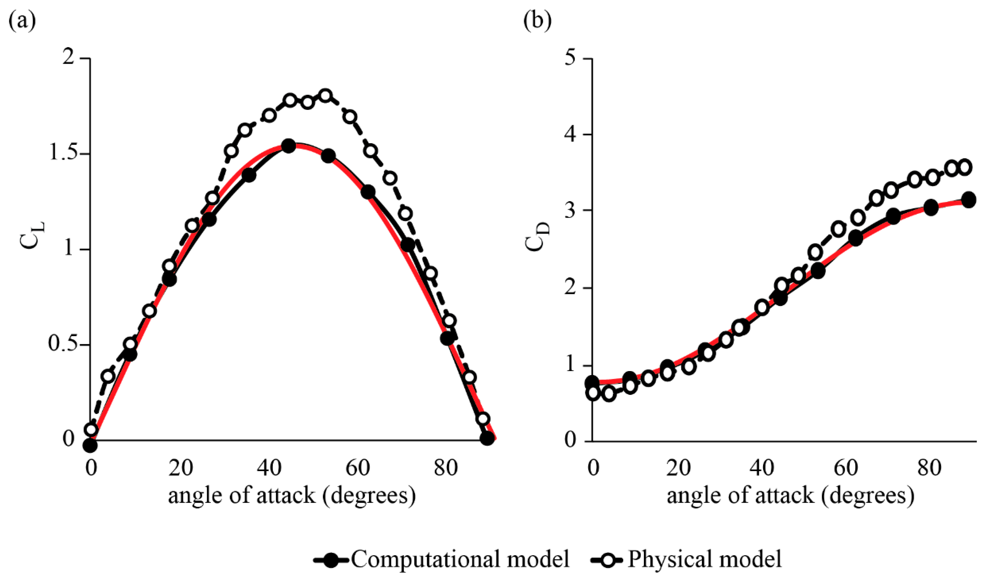
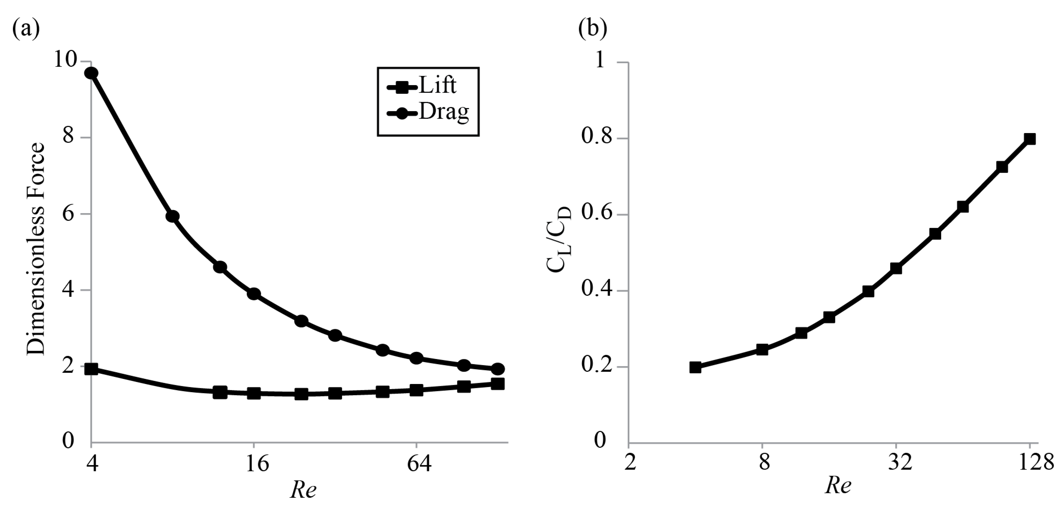
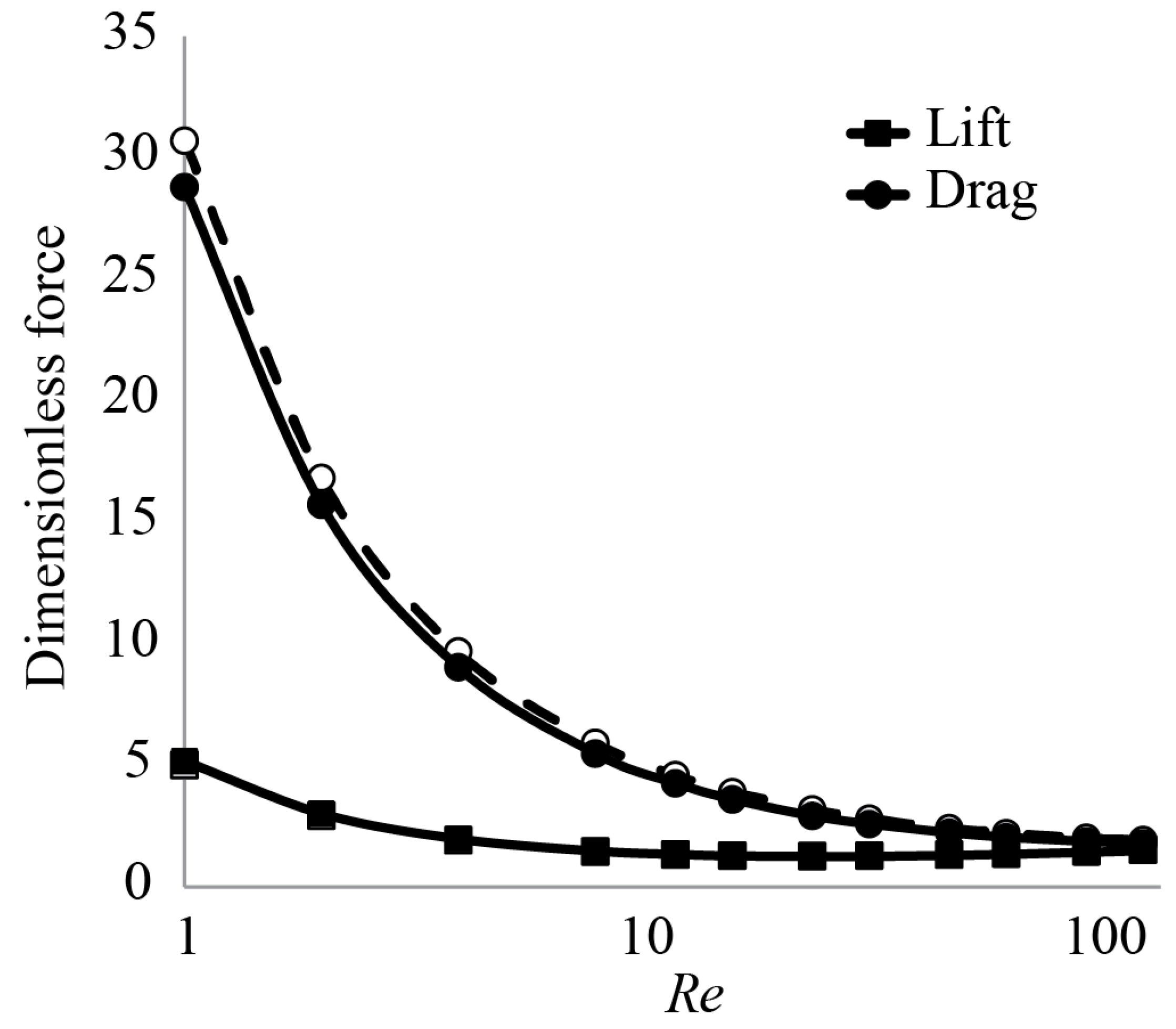
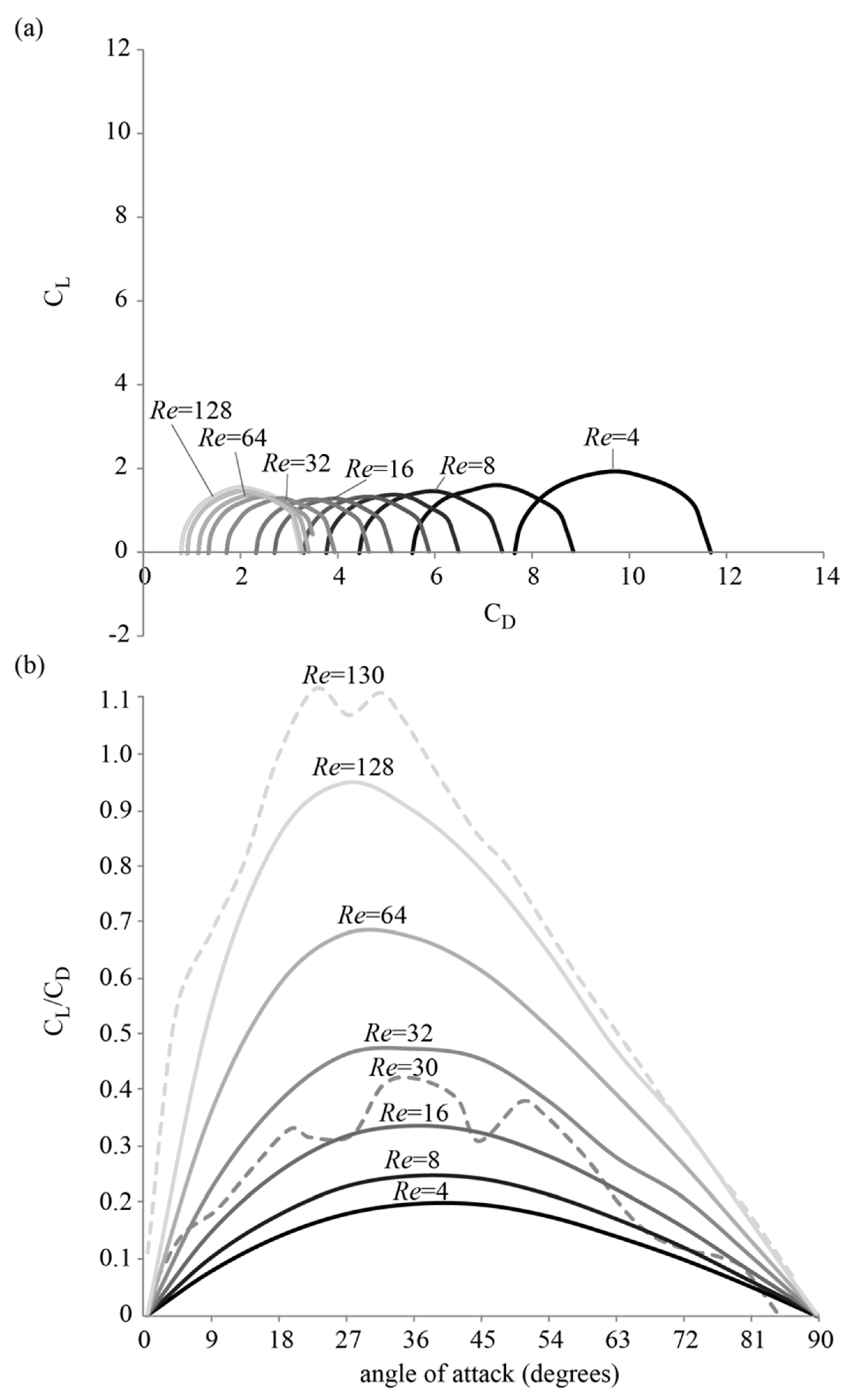
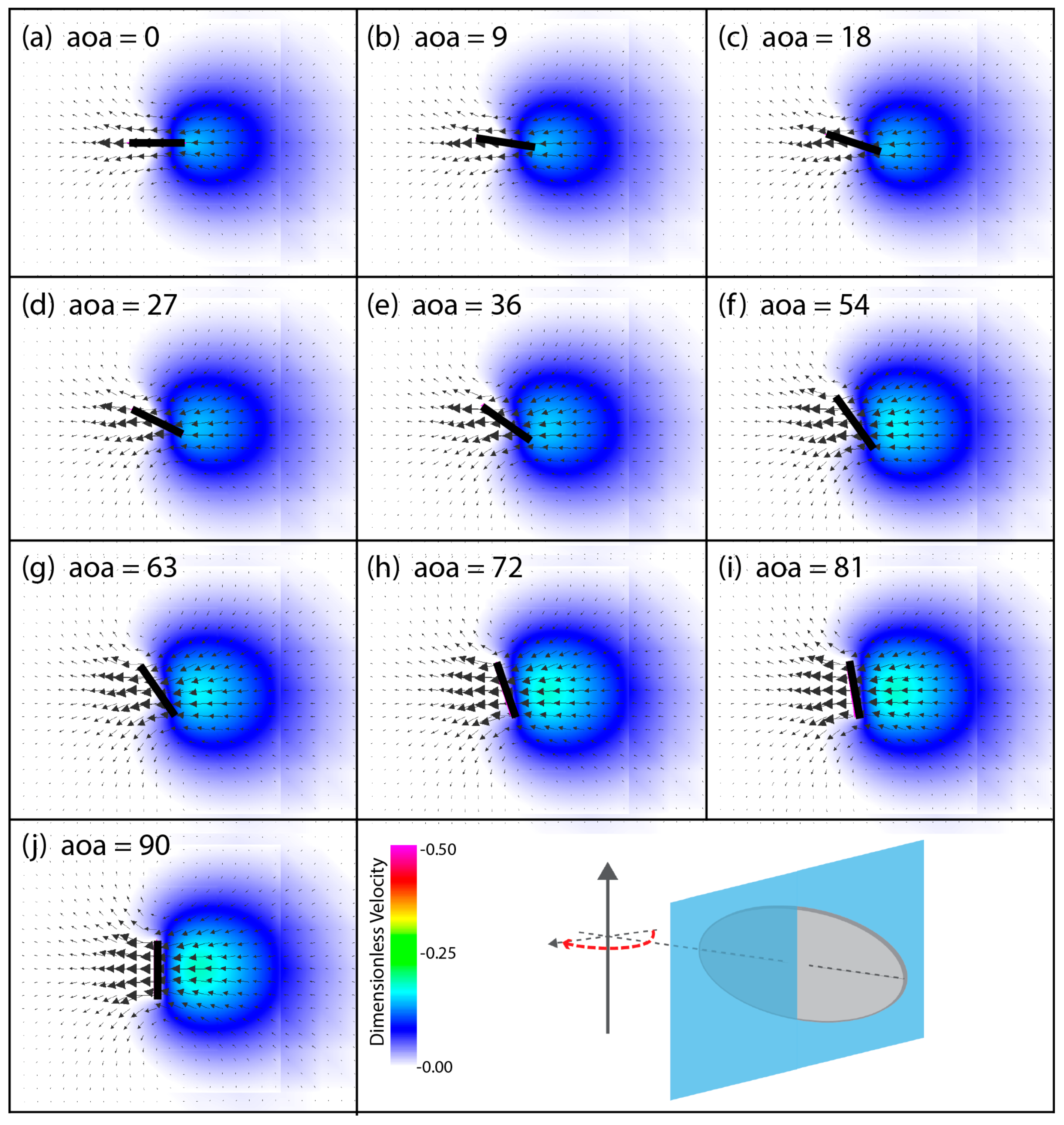
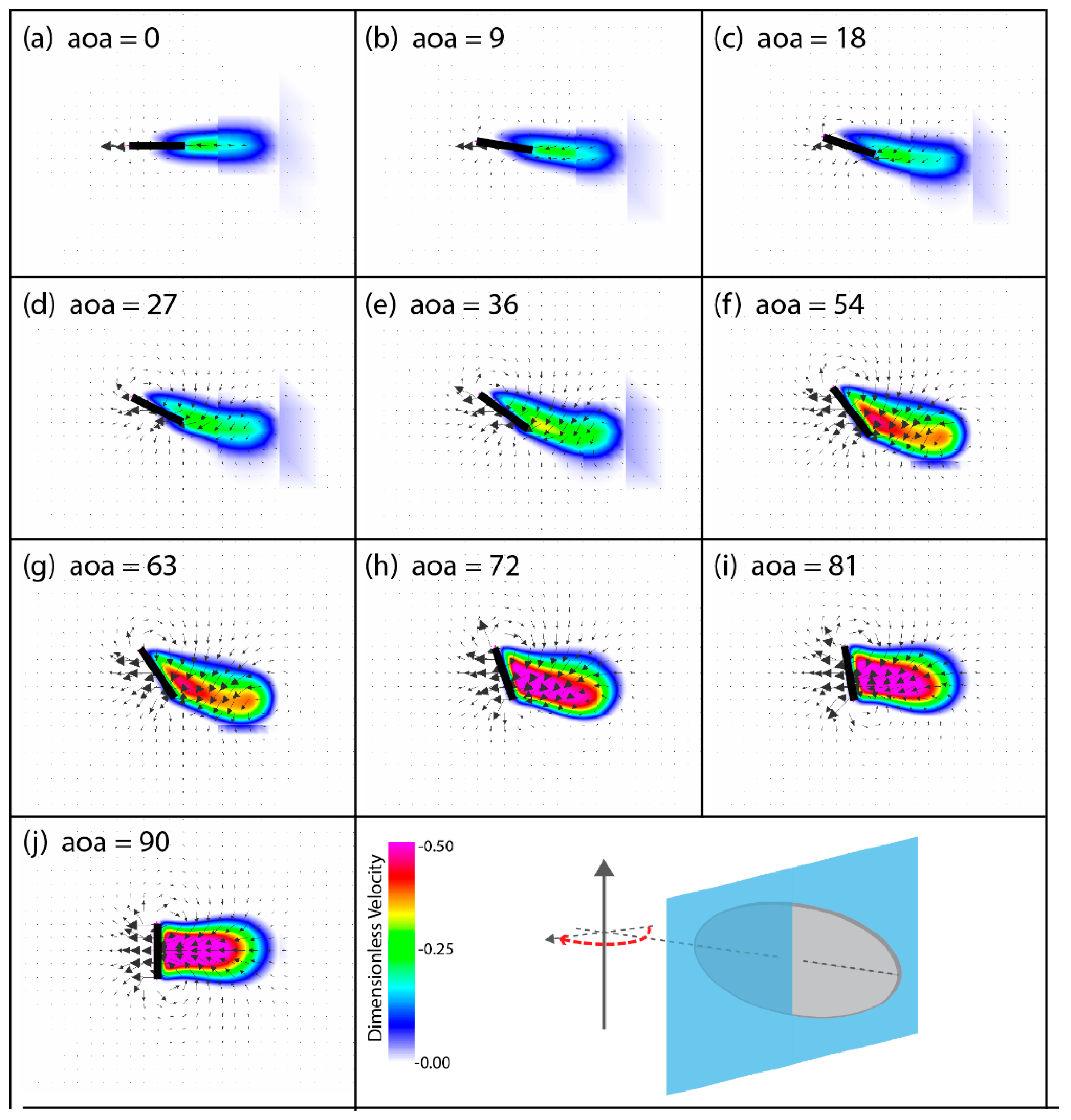
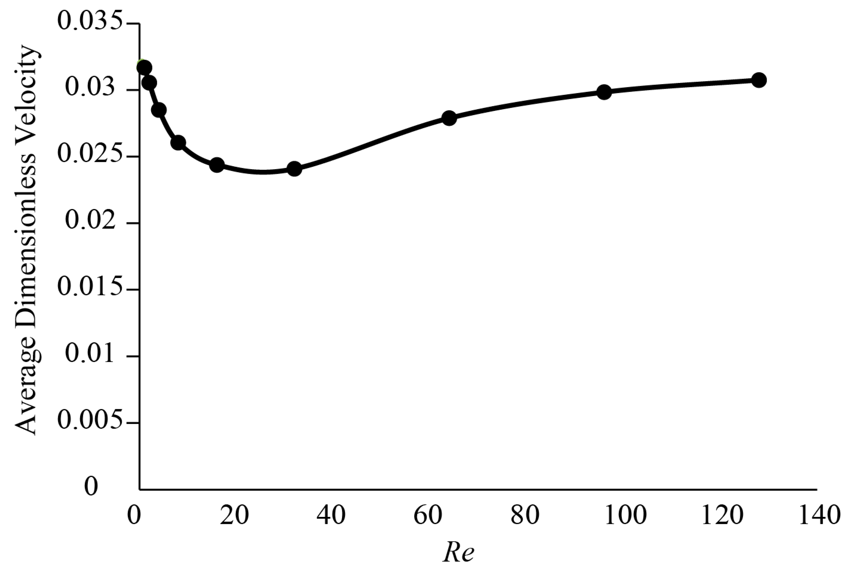
3.1. Forces around a Revolving Three-Dimensional Wing at Low Reynolds Numbers

The time-averaged lift and drag coefficients for the revolving physical and numerical model wings as functions of the angle of attack are shown in Figure 3 for Re = 130. The red lines show the quasi-steady force model described in Dickinson et al. [40] with coefficients selected for the computational model given as follows:

$$\begin{array}{l}{C}_L=0.18+1.36\sin \left(2.16\alpha -9.5\right),\\ C_D=2.0-1.2\cos \left(2.02\alpha -2.0\right).\end{array}$$

(3)

In general, there was good agreement between the computational and physical models; both results showed the same trends in forces generated as a function of Re and the angle of attack. The average difference between the physical and computational forces was <10%. The force sensor was not sensitive enough to measure forces at Re below 100, therefore, forces at lower Re are only shown for the computational model.

The results for Re = 130 were consistent with previously published results on a three-dimensional model of a flapping fruit fly wing [31,32,40]. The overall relationship between the force coefficients and angles of attack supported previous studies [31,53].

The forces shown in Figure 4a correspond to the steady motion of a revolving model wing at a fixed angle of attack of 45°, a value that is typical of the mid-stroke of most insects during hovering flight [38]. At the low Re applicable to thrips, drag coefficients rise to several times the values measured at higher Re, a result that has been seen in previous numerical studies [20]. The onset of the transition to highly elevated drag coefficients occurred near Re = 30. Note that an increase in the drag coefficient in this Re range is well known for many shapes including spheres and cylinders [54]. The lift coefficients also begin to increase for Re < 10, and this corresponds to larger net flux of fluid pushed downward by the wing (Figure A1).

Defined in terms of the average ratio of lift to drag (Figure 4b), flight becomes increasingly less efficient as Re decreases. The ratio of lift to drag at a 45° angle of attack approaches 1 for Re greater than 100, which agrees with previous results for fruit flies and larger insects [25,41,53,55,56]. The ratio of lift to drag approaches 0.2 for the smallest flying insects such as fairyflies and haplothrips. This is in agreement with previous studies that show that the ratio of lift to drag decreases significantly with decreasing Re [20,25].

The aerodynamic polars in Figure 5a show that while peak lift coefficient remained relatively constant, the plot shifted to the right with decreasing Re. This illustrates the sensitivity of the drag coefficient to Re at all angles of attack. The aerodynamic polar for Re = 128 was in good agreement with previous experimental models at Re = 110 [32] and Re = 120 [39]. Note that the drag was nonzero at a 0° angle of attack due to large viscous forces. Drag coefficients increased with increasing angle of attack. The maximum value of lift coefficient occurred at an angle of attack of 45° for all values of Re and increased slightly with increasing Re. Figure 5b shows a plot of the ratios of lift to drag as functions of angles of attack. At Re = 4, the peak ratio of lift to drag occurs at 45°. However, as the Re increases, the peak ratio of lift to drag occurs at lower angles of attack. Overall, these observations indicate that, at small scales, the aerodynamics of flapping insects is dominated by viscous drag.

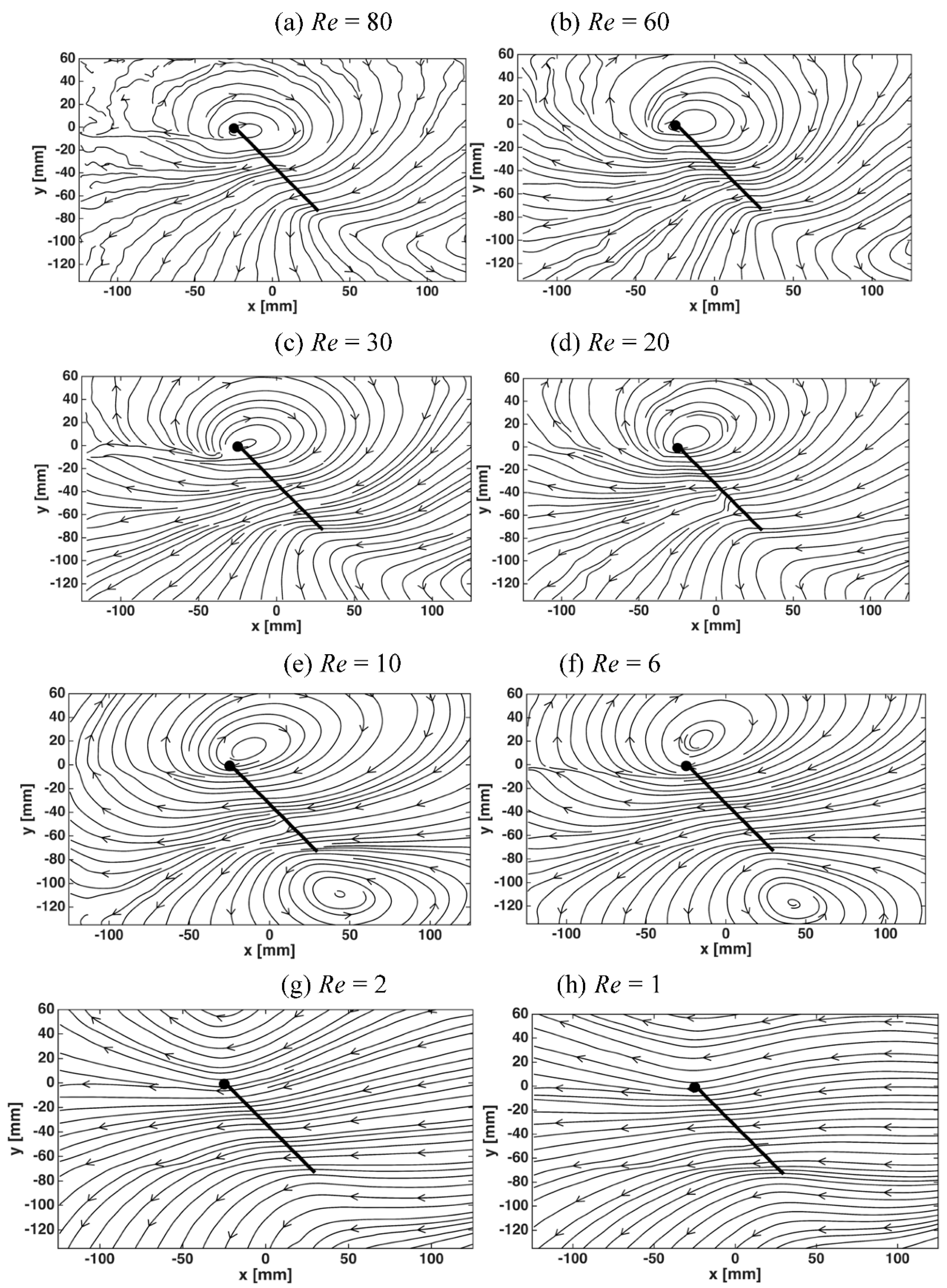
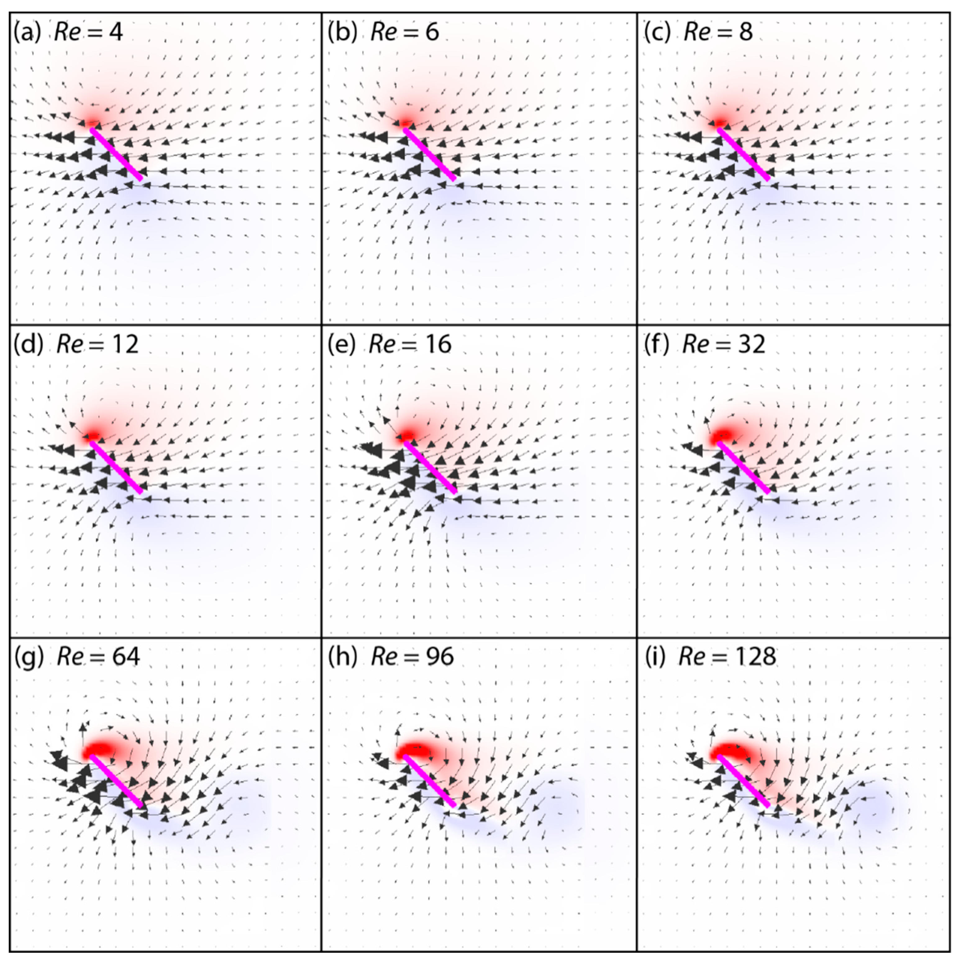
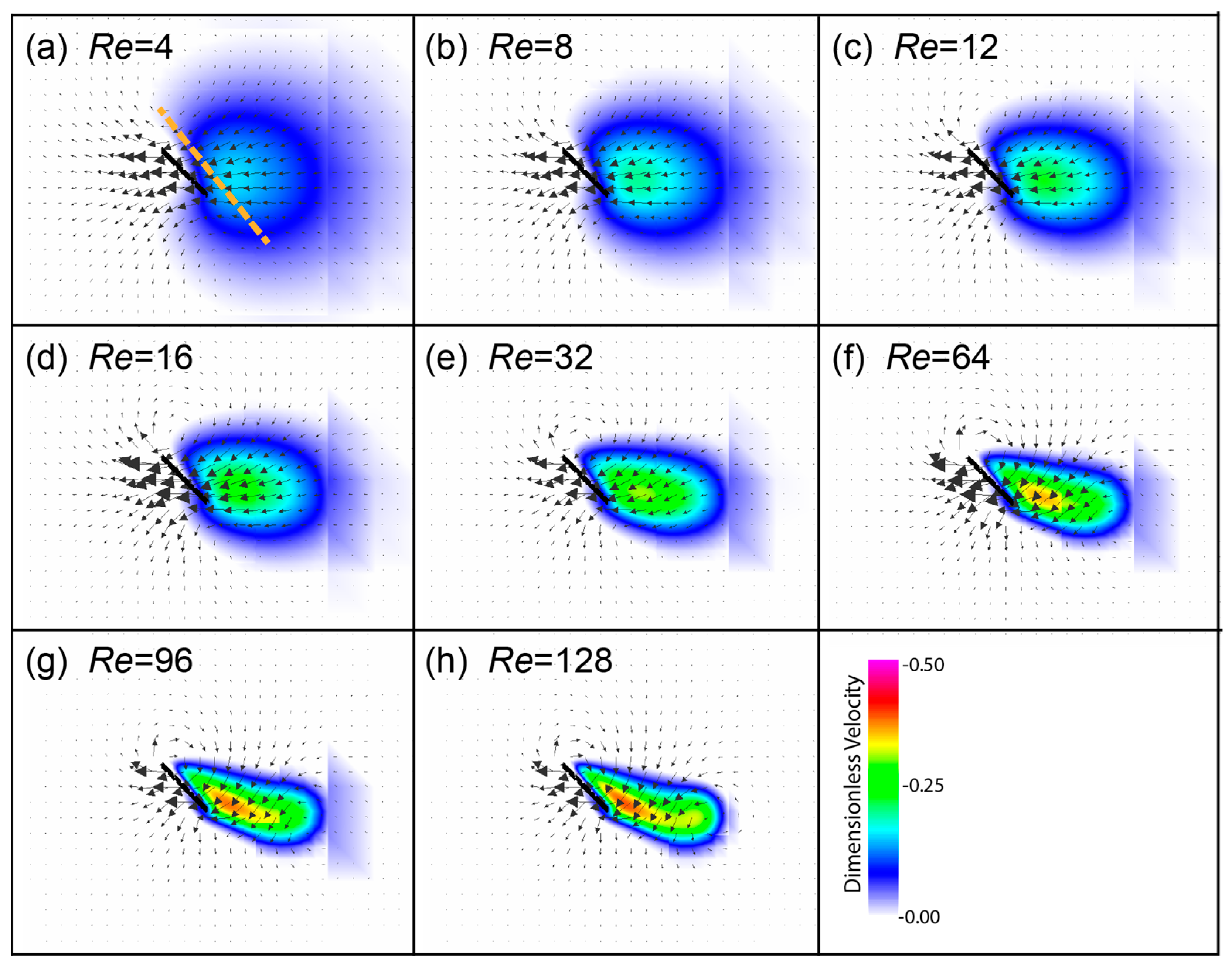
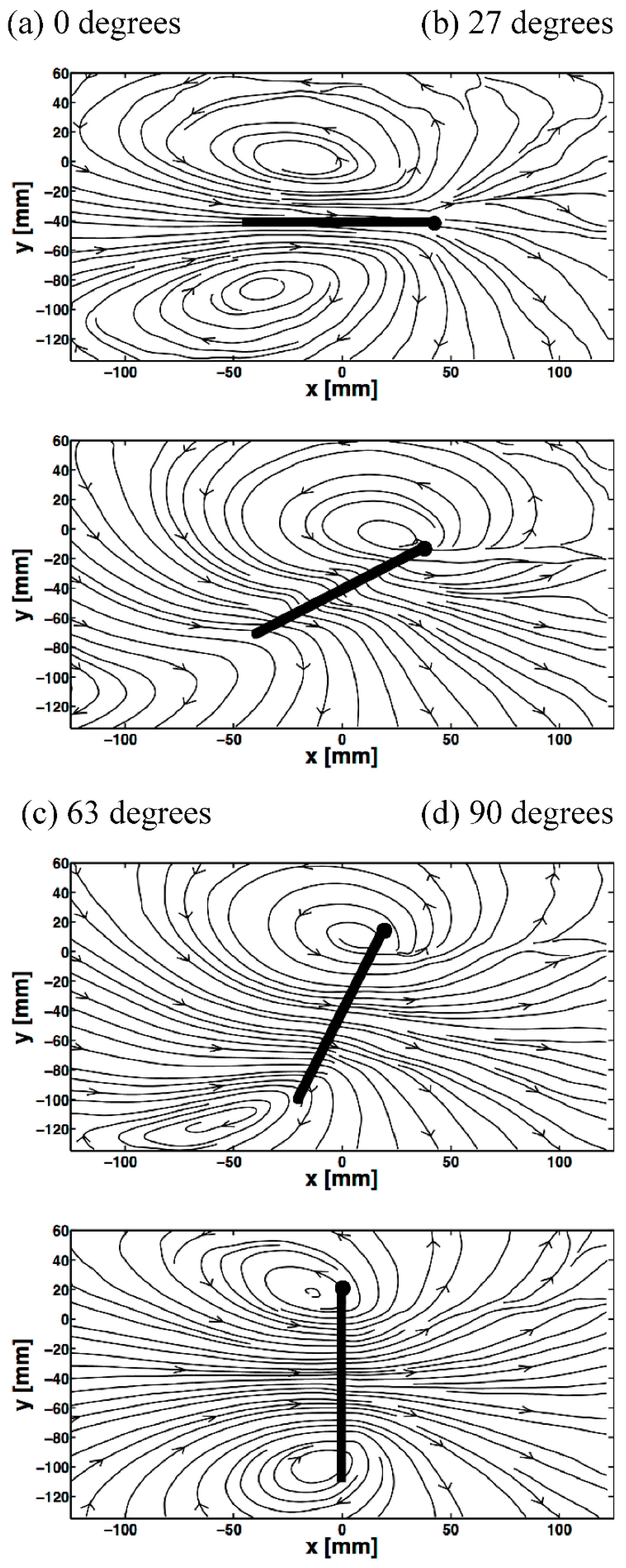
3.2. Flow Structures at Low Reynolds Numbers

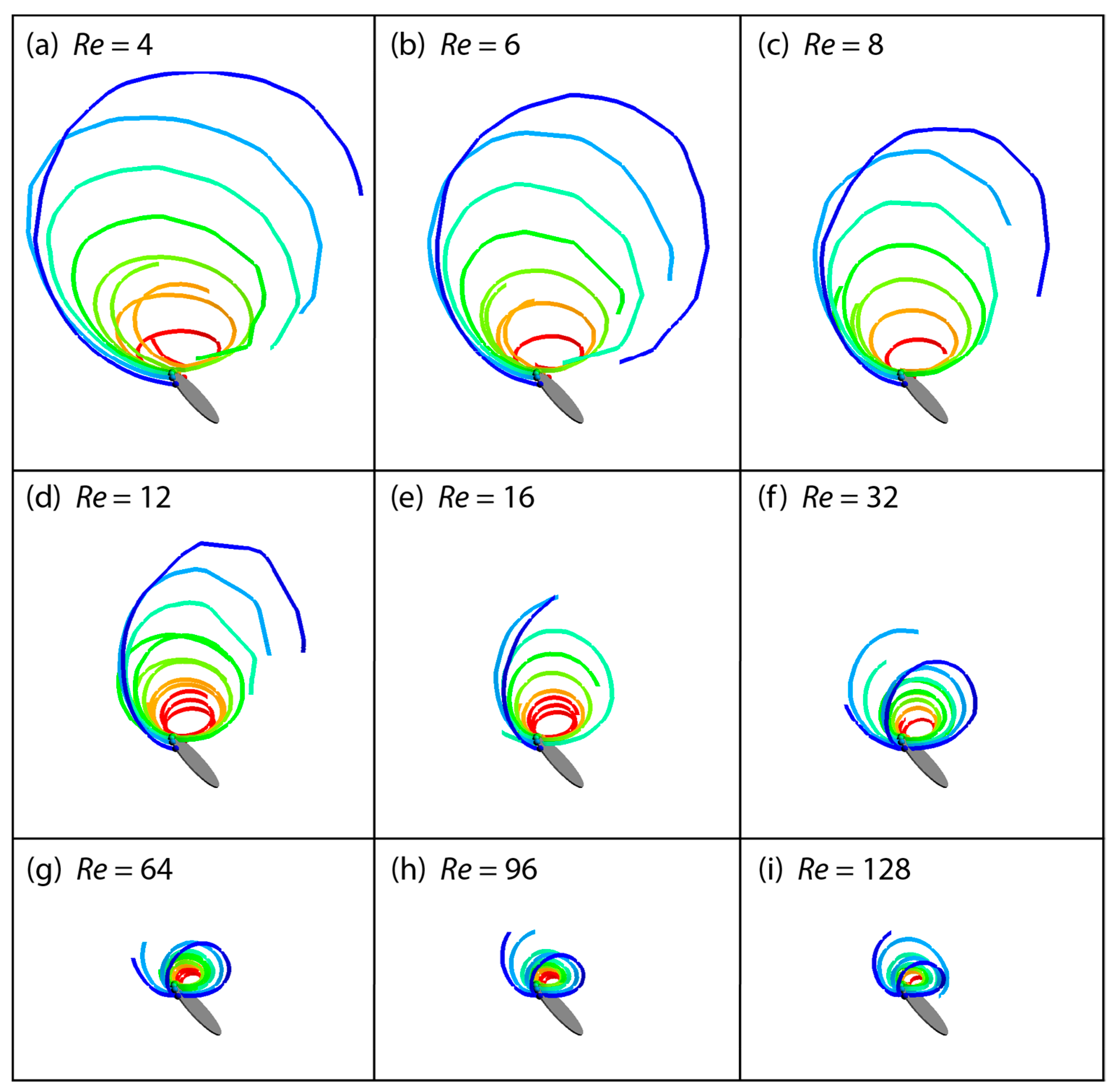
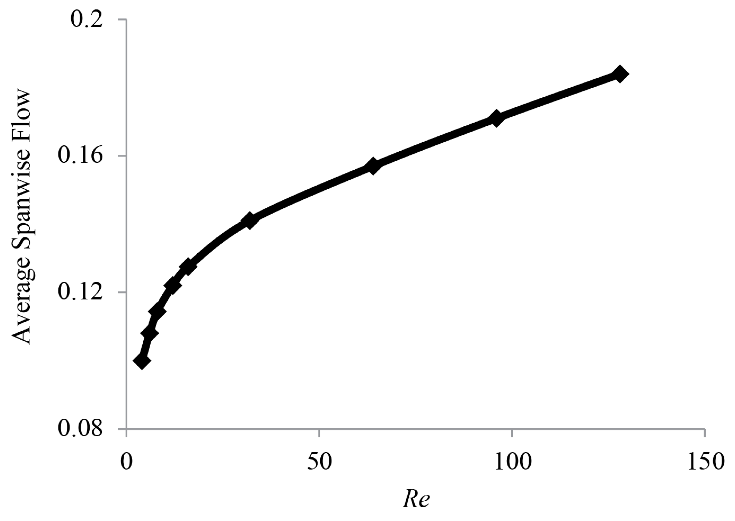
The effect of changing Re on the flow structure around the wing can be conveniently examined from the streamlines plotted for the physical (Figure 6) and computational model (Figure 7). The flow fields shown corresponds to the instant when the wing had swept 90° from its starting position at an angle of attack of 45°. For the physical model (Figure 6), the streamlines are instantaneous curves tangent to the local fluid velocity at every point in the vector flow field. Similarly, the streamlines for the computational model (Figure 7) are instantaneous curves that begin at seed locations along the leading edge of the wing and are tangential to the local fluid velocity at every point in the vector field. Each streamline was computed by a Runge-Kutta based numerical integration of the seed location through the vector field.

At higher Re, closer to the dynamic scale of fruit flies, an attached leading edge vortex (LEV) was observed at mid-stroke (Figure 6a and Figure 7i), as has been well-described in previous studies [31,39,40,57]. The corresponding trailing edge vortex (TEV) is shed in the wake and is no longer attached to the trailing edge at mid-stroke. It is not visible in the region of the flow field shown. The attached LEV is primarily responsible for delayed stall and enhanced lift generation [20,40,58]. The LEV, if formed, remained attached to the wing throughout the range of Re considered.

The computational results showed that as the Re is decreased from 128 to 4, the relative speed at which the TEV is advected into the wake also decreases (Figure 8). Note that the TEV appears closer to the wing for lower Re. As the relative effect of viscosity increases, the TEV is trapped in the larger boundary layer of the wing for longer periods of time and is effectively pulled along with the wing. At a Re range of from 4 to 32, which is representative of the range of flight experienced by the smallest insects, both the LEV and TEV did not separate from the wing (Figure 8a–f). The TEV was not shed into the wake at this range of Re due to the increased viscous forces present in the flow field that stabilize the vortex. This ‘vortical symmetry’ is in agreement with numerical results of Miller and Peskin [20] for two-dimensional wings. With decreasing Re and correspondingly reduced kinetic energy of the flow, both the LEV and TEV were more diffuse. In the experimental case for Re = 1 and 2, the TEV is rather diffuse and is not discernible within the visualized region of flow. The lack of separation of the TEV resulted in an overall reduction in the bound circulation around the wing.

3.3. Spanwise Flow

An advantage of performing three-dimensional computational studies is that we can readily obtain detailed information on spanwise flow and three-dimensional flow structures. In Figure 9, two-dimensional velocity vectors are shown in a plane that slices through a cross-section of the wing. A pseudocolor plot of the spanwise velocity (in a direction normal to the plane) is also provided to illustrate the three-dimensionality of the flow. Figure S1 shows a top-down view of a pseudocolor plot of the spanwise flow through a slice just above the wing. At Re = 4 (Figure 8a and Figure S1a), spanwise flow occurred over a broad region behind the wing. As the Re increased, the magnitude of the spanwise flow increased, and the region of non-negligible spanwise flow became smaller. Figure 9 also shows that the shape of the region of spanwise flow became more elongated as Re increases. The size and shape of the region of spanwise flow at Re = 128 matched a previous experimental study at Re = 120 [39] and a computational study at Re = 120 [59].

Figure 9 and Figure S1 show that maximum spanwise flow occurred farther behind the wing as the Re decreased. This is in agreement with the results of a previous experimental study [39] which found similar results comparing Re = 120 and Re = 1400, and the results of a computational study [59], which found similar results comparing Re = 120 and Re = 1500. Figure 9 shows that there was little spanwise flow in the LEV at Re < 128, which is also supported by previous experimental studies [32,39,59]. In a numerical study, Aono et al. [60] showed that spanwise flow was primarily confined to the core of the LEV at Re = 6300, but little spanwise flow existed in the LEV at Re = 134.

Figure 10 shows the average spanwise flow for a range of Re (angle of attack = 45°) calculated along the dashed transect shown in Figure 9a. The average spanwise flow increased with increasing Re, which has been observed previously at Re > 100 [39,59,60]. The dependence of the average spanwise flow on Re was the most sensitive for lower Re, particularly Re < 20. For 40 < Re < 128, average spanwise flow increased linearly with Re. It is interesting to note that the most sensitive Re range also corresponded to the scales at which the TEV did not separate from the wing and where the drag coefficient became particularly sensitive to Re.

We also investigated how small changes in the angle of attack affected the three-dimensional flow structure at Re = 4 (Figure 11) and Re = 128 (Figure 12) using the computational model (flow visualization around the physical model at varying angles of attack for Re = 32 is available in Appendix C and Figure A2). Figure S2 shows the three-dimensional flow structure at the intermediate value of Re = 32. For all angles of attack, the spanwise flow increased and became more spatially concentrated as the Re increased. As expected, the flow field structure was symmetric for both 0° and 90° angles of attack at all Re. As the angle of attack increased from 0° to 90°, the magnitude of the spanwise velocity also increased and was greater at larger Re. At Re = 4, the maximum spanwise flow increased by only 42% between 0° and 90° angles of attack, whereas, at Re = 128, the maximum spanwise flow increased by 200%. At Re = 4, there was little change in the shape of the region of spanwise flow as the angle of attack increased, whereas at Re = 128, the shape of the region of spanwise flow was greatly influenced by the angle of attack. As the angle of attack increased from 0° (Figure 12a) to 45° (Figure 12i), the region of spanwise flow extended behind and below the wing. As the angle of attack increased from 45° to 90° (Figure 12j), the region of spanwise flow became symmetrical again, and no longer extended below the trailing edge of the wing.

4. Discussion

In this study, we quantified the flow structures and forces around a three-dimensional revolving wing at a range of angles of attack and at Re ranging from 4 to 128 for both a dynamically scaled physical model and three-dimensional numerical simulations. Note that we only considered the case of a single rigid wing engaged in steady translation. We did not consider more complicated kinematics or the effects of wing-wing interactions, such as clap and fling [12]. Clap and fling has been observed in tiny insects such as Encarsia formosa [12] and thrips [15], and it is believed to enhance lift by the formation of a large attached LEV [21,22,23,35,61,62,63,64,65,66,67,68]. A two-dimensional numerical study demonstrated that very large drag forces are required to fling the wings apart at Re relevant to the smallest flying insects [21], however, that force is reduced when the wings are flexible [22] or porous [11]. A logical future direction in the analysis of flight of the smallest insects would be an investigation of the three-dimensional forces and flow structures around flexible wings engaged in clap and fling at the Re relevant to tiny insects.

For a single wing undergoing steady translation, our results are that (1) as the Re decreased, drag increased significantly; (2) defined in terms of the average ratio of lift to drag, single wing flapping became increasingly less efficient as Re decreased; (3) at the range of flight experienced by the smallest insects (4 < Re < 32), both the LEV and TEV remain attached to the wing; and (4) spanwise flow decreased with decreasing Re, especially in the range relevant to the smallest flying insects. Overall, these observations highlight the substantive differences in the aerodynamics of flight at the scale of the smallest flying insects when compared to larger insects. Flight at this extremely small scale is clearly challenging, and fundamental differences in aerodynamics suggest alternate wing morphology and kinematics might be necessary.

Overall, our results support previous research showing that aerodynamic efficiency is lower for smaller insects [11,12,15,17,18,20,21,22,23,24,25]. At the smallest scales (Re < 10), both lift and drag coefficients increased as Re decreases. However, the drag coefficient was most sensitive to changes in Re; drag increased significantly with decreasing Re, whereas there were only small changes in lift. At the scale of fruit flies (Re ~ 100), the ratio of lift to drag approached 1 as seen both here (Figure 4b) and elsewhere [25,41,53]. The ratio of lift to drag approached 0.2 for the smallest insects such as fairyflies and haplothrips (Re < 10).

The TEV and LEV did not separate from the wing for Re < 32 (Figure 7 and Figure 8). This vortical symmetry at lower Re has implications for the aerodynamics. An asymmetric attached LEV and shed TEV has been shown to increase lift [20,36,58]. At a Re range of 4–32, which is representative of the range of flight experienced by the smallest insects, both the LEV and TEV did not separate from the wing due to the increased viscous forces present in the flow field that stabilize the TEV. For Re, between about 10 and 32, this results in an overall reduction in the bound circulation around the wing, and consequently a decrease in lift. Equivalently, the symmetric attached LEV and TEV reduced the time rate of change of the first moment of vorticity which is proportional to the lift acting on the wing [20].

Perhaps surprisingly, lift does begin to increase for Re < 10, though drag increases faster. This result is supported by an analysis of Oseen’s equations describing flow past an inclined elliptical cylinder in the classical paper of Imai [69]. He found that the lift coefficient for a flat plate at a 45-degree angle of attack increased from about 2.9 at Re = 1 to about 6.9 at Re = 0.1. This result was later supported by In et al. [70] who numerically solved the Navier-Stokes equations of the vorticity-stream function in body-fitted coordinates for the steady flow past an inclined elliptical cylinder. They found that the lift coefficient increased from about 1.2 to 2 as the Re was lowered from 10 to 1. The physical intuition for this phenomenon is not immediately obvious, and it is likely that circulation based arguments for lift generation are not relevant at these Re. Some intuition may be gained by noticing that the flow does not separate from the wing tips for Re < 4 and moves smoothly over and under the wing. As a result of the inclination, the net movement of fluid is downward, creating an upward force on the wing. Due to the increased boundary layer at lower Re, an increased volume of fluid is deflected downward. This trend is quantified in Figure A1 which shows the net flux of fluid pushed downward as a function of Re.

Using the computational model, we also quantified spanwise flow along the rotating wing. Our results showed that as Re decreases, the magnitude of spanwise flow decreased, whereas the region over which it occurs behind the wing broadens (Figure 9). In larger insects such as hawkmoths, the spanwise flow is concentrated in the LEV [60]. Our numerical results showed that there was little spanwise flow in the LEV at Re < 128, which is in agreement with previous experimental studies [32,39,59] and numerical studies [17,60]. The shape of the region of non-negligible spanwise flow also changed with Re. At Re = 4 (Figure 9a), a cross-section of the region of spanwise flow behind the wing was round and symmetrical. As the Re increased, however, the region became elongated and began to extend behind and below the wing. At Re = 128 (Figure 9h), the shape of the region of spanwise flow was in agreement with previous experimental studies [39,59].

The major difference between two-dimensional computations and three-dimensional insect wings is the presence of spanwise flow and its consequences on vortex dynamics [31]. For example, the LEV is shed after traveling a few chord lengths in two-dimensional models [20,53], whereas the LEV remains stably attached to a revolving three-dimensional wing for much longer distances [31,40]. For the LEV to remain attached to the wing, the following three processes should be balanced: the advection of the vortex, the intensification of vorticity due to vortex stretching, and the diffusion of vorticity by viscosity. In this case, vortex stretching is observed through the spanwise flow. As the Re is lowered, spanwise flow is reduced while vortex diffusion is enhanced. In the two-dimensional case, vortex stretching cannot occur. The patterns of vortex shedding at low Re in this three-dimensional study were in good agreement with the numerical results of a two-dimensional wing [20]. This suggests that the diffusion of vorticity is sufficient to stabilize the LEV in the flight of the smallest insects. Moreover, two-dimensional studies may more accurately model small insect flight than large insect flight.

Finally, the question remains as to how tiny insects are able to generate sufficient lift to stay aloft. To fully address this question, we need better data on wingbeat kinematics and more detailed numerical or physical models that consider wing-wing interaction. To estimate whether or not a single wing in steady translation can generate sufficient lift, we can consider the case of the chalcid wasp, Encarsia formosa. This insect has a total mass of about $2.5\times {10}^{-8}$ kg, a wingbeat frequency of 370 Hz, and a wing length of $7.0\times {10}^{-4}$ m [12]. We will also assume a lift coefficient of 1.3, stroke amplitude of $2\mathsf{\pi }/3$ radians, an elliptical wing shape, and a maximum chord of $4.7\times {10}^{-4}$ m. Using Equation (2) with ${\widehat{r}}_2^2$(S) = 0.38, we obtain a lift force of $1.17\times {10}^{-7}$ N, and the lift generated by two wings that do not interact aerodynamically would be $2.34\times {10}^{-7}$ N. The gravitational force acting on the insect is about $2.45\times {10}^{-7}$ N, suggesting the lift augmentation due to unsteady mechanisms and wing-wing interaction is important for maintaining altitude, accelerating upwards, and carrying any additional load.

References

1. Huber, J.T.; Noyes, J.S. A new genus and species of fairyfly, Tinkerbella nana (Hymenoptera, Mymaridae), with comments on its sister genus Kikiki, and discussion on small size limits in arthropods. J. Hymenopt. Res. 2013, 32, 17–44. [Google Scholar] [CrossRef]
2. Palmer, J.M.; Reddy, D.V.R.; Wightman, J.A.; Rao, G.V.R. New information on the thrips vectors of tomato spotted wilt virus in groundnut crops in India. Int. Arachis Newsl. 1990, 7, 24–25. [Google Scholar]
3. Crespi, B.J.; Carmean, D.A.; Chapman, T.W. Ecology and evolution of galling thrips and their allies. Annu. Rev. Entomol. 1997, 42, 51–71. [Google Scholar] [CrossRef] [PubMed]
4. Austin, A.; Dowton, M. Hymenoptera: Evolution, Biodiversity and Biological Control; Csiro Publishing: Clayton, Australia, 2000. [Google Scholar]
5. Strickland, C.; Kristensen, N.P.; Miller, L.A. Inferring stratified parasitoid dispersal mechanisms and parameters from coarse data using mathematical and Bayesian methods. R. Soc. Interface 2017, 215, 2369–2381. [Google Scholar] [CrossRef] [PubMed]
6. Shogren, C.; Paine, T.D. Economic Benefit for Cuban Laurel Thrips Biological Control. J. Econ. Entomol. 2016, 109, 93–99. [Google Scholar] [CrossRef] [PubMed]
7. Terry, I. Thrips and weevils as dual, specialist pollinators of the Australian cycad Macrozamia communis (Zamiaceae). Int. J. Plant Sci. 2001, 162, 1293–1305. [Google Scholar] [CrossRef]
8. Terry, I. Thrips: The primeval pollinators. In Thrips and Tospoviruses: Proceedings of the 7th International Symposium on Thysanoptera, Calabria, Italy, 2–7 July 2001; Australian National Insect Collection: Canberra, Australia, 2002. [Google Scholar]
9. Jones, D.R. Plant viruses transmitted by thrips. Eur. J. Plant Pathol. 2005, 113, 119–157. [Google Scholar] [CrossRef]
10. Ullman, D.E.; Meideros, R.; Campbell, L.R.; Whitfield, A.E.; Sherwood, J.L.; German, T.L. Thrips as vectors of tospoviruses. Adv. Bot. Res. 2002, 36, 113–140. [Google Scholar]
11. Santhanakrishnan, A.; Robinson, A.K.; Jones, S.; Low, A.A.; Gadi, S.; Hedrick, T.L.; Miller, L.A. Clap and fling mechanism with interacting porous wings in tiny insect flight. J. Exp. Biol. 2014, 217, 3898–3909. [Google Scholar] [CrossRef] [PubMed] [Green Version]
12. Weis-Fogh, T. Quick estimates of flight fitness in hovering animals, including novel mechanisms for lift production. J. Exp. Biol. 1973, 59, 169–230. [Google Scholar]
13. Bomphrey, R.J.; Nakata, T.; Phillips, N.; Walker, S.W. Smart wing rotation and trailing-edge vortices enable high frequency mosquito flight. Nature 2017, 544, 92–95. [Google Scholar] [CrossRef] [PubMed] [Green Version]
14. Davidi, G.; Weihs, D. Flow around a Comb Wing in Low-Reynolds-Number Flow. AIAA J. 2012, 50, 249–253. [Google Scholar] [CrossRef]
15. Ellington, C.P. Wing mechanics and take-off preparation of Thrips (Thysanoptera). J. Exp. Biol. 1980, 85, 129–136. [Google Scholar]
16. Jones, S.K.; Yun, Y.J.; Hedrick, T.L.; Griffith, B.E.; Miller, L.A. Bristles reduce the force required to ‘fling’ wings apart in the smallest insects. J. Exp. Biol. 2016, 219, 3759–3772. [Google Scholar] [CrossRef] [PubMed] [Green Version]
17. Kolomenskiy, D.; Moffatt, H.; Farge, M.; Schneider, K. Two-and three-dimensional numerical simulations of the clap–fling–sweep of hovering insects. J. Fluids Struct. 2011, 27, 784–791. [Google Scholar] [CrossRef]
18. Kolomenskiy, D.; Moffatt, H.K.; Farge, M.; Schneider, K. Vorticity generation during the clap–fling–sweep of some hovering insects. Theor. Comput. Fluid Dyn. 2010, 24, 209–215. [Google Scholar] [CrossRef]
19. Lee, S.H.; Kim, D. Aerodynamics of a translating comb-like plate inspired by a fairyfly wing. Phys. Fluids 2017, 29, 081902. [Google Scholar] [CrossRef]
20. Miller, L.A.; Peskin, C.S. When vortices stick: An aerodynamic transition in tiny insect flight. J. Exp. Biol. 2004, 207, 3073–3088. [Google Scholar] [CrossRef] [PubMed]
21. Miller, L.A.; Peskin, C.S. A computational fluid dynamics study of ’clap and fling’ in the smallest insects. J. Exp. Biol. 2005, 208, 17. [Google Scholar] [CrossRef] [PubMed]
22. Miller, L.A.; Peskin, C.S. Flexible clap and fling in tiny insect flight. J. Exp. Biol. 2009, 212, 3076–3090. [Google Scholar] [CrossRef] [PubMed] [Green Version]
23. Sun, M.; Yu, X. Aerodynamic force generation in hovering flight in a tiny insect. AIAA J. 2006, 44, 1532–1540. [Google Scholar] [CrossRef]
24. Sunada, S.; Takashima, H.; Hattori, T.; Yasuda, K.; Kawachi, K. Fluid-dynamic characteristics of a bristled wing. J. Exp. Biol. 2002, 205, 2737–2744. [Google Scholar] [PubMed]
25. Wang, Z.J. Two dimensional mechanism for insect hovering. Phys. Rev. Lett. 2004, 85, 2216–2219. [Google Scholar] [CrossRef] [PubMed]
26. Wang, Z.J. The role of drag in insect hovering. J. Exp. Biol. 2004, 207, 4147–4155. [Google Scholar] [CrossRef] [PubMed] [Green Version]
27. Żbikowski, R. On aerodynamic modelling of an insect–like flapping wing in hover for micro air vehicles. Philos. Trans. R. Soc. Lond. A Math. Phys. Eng. Sci. 2002, 360, 273–290. [Google Scholar] [CrossRef] [PubMed]
28. Wu, J.H.; Sun, M. Unsteady aerodynamic forces of a flapping wing. J. Exp. Biol. 2004, 207, 1137–1150. [Google Scholar] [CrossRef] [PubMed] [Green Version]
29. Arora, N.; Gupta, A.; Sanghi, S.; Aono, H.; Shyy, W. Lift-drag and flow structures associated with the “clap and fling” motion. Phys. Fluids 2014, 26, 071906. [Google Scholar] [CrossRef]
30. Jones, S.; Laurenza, R.; Hedrick, T.L.; Griffith, B.E.; Miller, L.A. Lift vs. drag based mechanisms for vertical force production in the smallest flying insects. J. Theor. Biol. 2015, 384, 105–120. [Google Scholar] [CrossRef] [PubMed] [Green Version]
31. Wang, Z.J.; Birch, J.M.; Dickinson, M.H. Unsteady forces and flows in low Reynolds number hovering flight: Two-dimensional computations vs robotic wing experiments. J. Exp. Biol. 2004, 207, 449–460. [Google Scholar] [CrossRef] [PubMed]
32. Lentink, D.; Dickinson, M.H. Rotational accelerations stabilize leading edge vortices on revolving fly wings. J. Exp. Biol. 2009, 212, 2705–2719. [Google Scholar] [CrossRef] [PubMed] [Green Version]
33. Liu, H.; Aono, H. Size effects on insect hovering aerodynamics: An integrated computational study. Bioinspir. Biomim. 2009, 4, 015002. [Google Scholar] [CrossRef] [PubMed]
34. Chin, D.D.; Lentink, D. Flapping wing aerodynamics: From insects to vertebrates. J. Exp. Biol. 2016, 219, 920–932. [Google Scholar] [CrossRef] [PubMed]
35. Ellington, C.P. The aerodynamics of hovering insect flight. III. Kinematics. Philos. Trans. R. Soc. Lond. B Biol. Sci. 1984, 305, 41–78. [Google Scholar] [CrossRef]
36. Ellington, C.P. The novel aerodynamics of insect flight: Applications to micro-air vehicles. J. Exp. Biol. 1999, 202, 3439–3448. [Google Scholar] [PubMed]
37. Hedrick, T.L.; Combes, S.; Miller, L.A. Recent developments in the study of insect flight. Can. J. Zool. 2015, 92, 3898–3909. [Google Scholar] [CrossRef]
38. Sane, S.P. The aerodynamics of insect flight. J. Exp. Biol. 2003, 206, 4191–4208. [Google Scholar] [CrossRef] [PubMed] [Green Version]
39. Birch, J.M.; Dickson, W.B.; Dickinson, M.H. Force production and flow structure of the leading edge vortex on flapping wings at high and low Reynolds numbers. J. Exp. Biol. 2004, 207, 1063–1072. [Google Scholar] [CrossRef] [PubMed] [Green Version]
40. Dickinson, M.H.; Lehmann, F.-O.; Sane, S.P. Wing rotation and the aerodynamic basis of insect flight. Science 1999, 284, 1954–1960. [Google Scholar] [CrossRef] [PubMed]
41. Sane, S.P.; Dickinson, M.H. The control of flight force by a flapping wing: Lift and drag production. J. Exp. Biol. 2001, 204, 2607–2626. [Google Scholar] [PubMed]
42. Fauci, L.J.; Fogelson, A.L. Truncated Newton methods and the modeling of complex immersed elastic structures. Commun. Pure Appl. Math. 1993, 46, 787–818. [Google Scholar] [CrossRef]
43. Fauci, L.J.; Peskin, C.S. A computational model of aquatic animal locomotion. J. Comput. Phys. 1988, 77, 85–108. [Google Scholar] [CrossRef]
44. Herschlag, G.; Miller, L. Reynolds number limits for jet propulsion: A numerical study of simplified jellyfish. J. Theor. Biol. 2011, 285, 84–95. [Google Scholar] [CrossRef] [PubMed] [Green Version]
45. Griffith, B.E.; Luo, X. Hybrid finite difference/finite element version of the immersed boundary method. Int. J. Numer. Methods Biomed. Eng. 2017, 33, e2888. [Google Scholar] [CrossRef] [PubMed]
46. Geuzaine, C.; Remacle, J.F. Gmsh: A 3-D finite element mesh generator with built-in pre-and post-processing facilities. Int. J. Numer. Methods Eng. 2009, 79, 1309–1331. [Google Scholar] [CrossRef]
47. Griffith, B.E.; Hornung, R.D.; McQueen, D.M.; Peskin, C.S. An adaptive, formally second order accurate version of the immersed boundary method. J. Comput. Phys. 2007, 223, 10–49. [Google Scholar] [CrossRef] [Green Version]
48. Nguyen, H.; Karp-Boss, L.; Jumars, P.A.; Fauci, L. Hydrodynamic effects of spines: A different spin. Limnol. Oceanogr. Fluids Environ. 2011, 1, 110–119. [Google Scholar] [CrossRef] [Green Version]
49. Vo, G.D.; Heys, J. Biofilm Deformation in Response to Fluid Flow in Capillaries. Biotechnol. Bioeng. 2011, 108, 1893–1899. [Google Scholar] [CrossRef] [PubMed]
50. Tytell, E.D.; Hsu, C.Y.; Williams, T.L.; Cohen, A.H.; Fauci, L.J. Interactions between internal forces, body stiffness, and fluid environment in a neuromechanical model of lamprey swimming. Proc. Natl. Acad. Sci. USA 2010, 107, 19832–19837. [Google Scholar] [CrossRef] [PubMed] [Green Version]
51. Griffith, B.E. Immersed boundary model of aortic heart valve dynamics with physiological driving and loading conditions. Int. J. Numer. Methods Biomed. Eng. 2012, 28, 317–345. [Google Scholar] [CrossRef]
52. Griffith, B.E.; Luo, X.Y.; McQueen, D.M.; Peskin, C.S. Simulating the fluid dynamics of natural and prosthetic heart valves using the immersed boundary method. Int. J. Appl. Mech. 2009, 1, 137–177. [Google Scholar] [CrossRef]
53. Dickinson, M.H.; Gotz, K.G. Unsteady aerodynamic performance of model wings at low Reynolds numbers. J. Exp. Biol. 1993, 174, 45–64. [Google Scholar]
54. Batchelor, G. An Introduction to Fluid Dynamics. Cambridge Mathematical Library, 2nd ed.; Cambridge University Press: Cambridge, UK, 2000; ISBN 978-0-521-66396-0. [Google Scholar]
55. Usherwood, J.R.; Ellington, C.P. The aerodynamics of revolving wings: I. Model hawkmoth wings. J. Exp. Biol. 2002, 205, 1547–1564. [Google Scholar] [PubMed]
56. Usherwood, J.R.; Ellington, C.P. The aerodynamics of revolving wings: II. Propeller force coefficients from mayfly to quail. J. Exp. Biol. 2002, 205, 1565–1576. [Google Scholar] [PubMed]
57. Ellington, C.P.; van den Berg, C.; Willmott, A.P.; Thomas, A.L. Leading-edge vortices in insect flight. Nature 1996, 384, 626–630. [Google Scholar] [CrossRef]
58. Birch, J.M.; Dickinson, M.H. Spanwise flow and the attachment of the leading-edge vortex on insect wings. Nature 2001, 412, 729–733. [Google Scholar] [CrossRef] [PubMed]
59. Harbig, R.; Sheridan, J.; Thompson, M. Reynolds number and aspect ratio effects on the leading-edge vortex for rotating insect wing planforms. J. Fluid Mech. 2013, 717, 166–192. [Google Scholar] [CrossRef]
60. Aono, H.; Liang, F.; Liu, H. Near-and far-field aerodynamics in insect hovering flight: An integrated computational study. J. Exp. Biol. 2008, 211, 239–257. [Google Scholar] [CrossRef] [PubMed]
61. Ellington, C.P. The aerodynamics of hovering insect flight. IV. Aerodynamic mechanisms. Philos. Trans. R. Soc. Lond. B Biol. Sci. 1984, 305, 79–113. [Google Scholar] [CrossRef]
62. Lehmann, F.O.; Pick, S. The aerodynamic benefit of wing-wing interaction depends on stroke trajectory in flapping insect wings. J. Exp. Biol. 2007, 210, 1362–1377. [Google Scholar] [CrossRef] [PubMed] [Green Version]
63. Lehmann, F.O.; Sane, S.P.; Dickinson, M. The aerodynamic effects of wing-wing interaction in flapping insect wings. J. Exp. Biol. 2005, 208, 3075–3092. [Google Scholar] [CrossRef] [PubMed] [Green Version]
64. Lighthill, M.J. On the Weis-Fogh mechanism of lift generation. J. Fluid Mech. 1973, 60, 1–17. [Google Scholar] [CrossRef]
65. Maxworthy, T. Experiments on the Weis-Fogh mechanism of lift generation by insects in hovering flight. Part 1. Dynamics of the fling. J. Fluid Mech. 1979, 93, 47–63. [Google Scholar] [CrossRef]
66. Spedding, G.R.; Maxworthy, T. The generation of circulation and lift in a rigid two-dimensional fling. J. Fluid Mech. 1986, 165, 247–272. [Google Scholar] [CrossRef]
67. Sun, M.; Xin, Y. Flows around two airfoils performing fling and subsequent translation and translation and subsequent clap. Acta Mech. Sin. 2003, 19, 13–117. [Google Scholar]
68. Ellington, C. The aerodynamics of hovering insect flight. I. The quasi-steady analysis. Philos. Trans. R. Soc. Lond. B Biol. Sci. 1984, 305, 1–15. [Google Scholar] [CrossRef]
69. Imai, I. A New Method of Solving Oseen’s Equations and Its Application to the Flow Past anInclined Elliptic Cylinder. Proc. R. Soc. Lond. Ser. A Math. Phys. Sci. 1954, 224, 141–160. [Google Scholar] [CrossRef]
70. In, K.M.; Choi, D.H.; Kim, M.-U. Two-dimensional viscous flow past a flat plate. Fluid Dyn. Res. 1995, 15, 13–24. [Google Scholar] [CrossRef]
Figure 1. The experimental setup. (a) The dynamically scaled wing was immersed in a clear 1 m × 1 m × 2 m plexiglass tank filled with mineral oil. Only a single wing was used in this study; (b) The wing was constructed from 2.0 mm thick clear acrylic sheet (c = 8.25 cm, b = 16.5 cm, and R = 20.1 cm) and revolved through a 180° arc in a horizontal stroke plane with constant angular velocity at a fixed angle of attack. Flow structure was visualized using two-dimensional digital particle image velocimetry (DPIV). The DPIV laser light sheet was oriented along the center of the wingspan.
Fluids 03 00045 g001
Figure 2. The refinement study comparing average dimensionless lift (squares) and drag (circles) over a range of Re at 2563 (open markers) and 5123 (solid markers) grid discretization. The average dimensionless force was calculated over the steady part of the stroke. Effective 2563 grid discretization was used for all other simulations in this study.
Fluids 03 00045 g002
Figure 3. The comparison of (a) lift and (b) drag for the computational (solid markers) and experimental (open markers) models over a range of angles of attack at Re = 130. The red lines show the quasi-steady force model described in Dickinson et al. [40].
Fluids 03 00045 g003
Figure 4. The average (a) dimensionless lift (squares) and drag (circles) and (b) the ratio of lift to drag over a range of Re (aoa = 45°). These results were obtained from three-dimensional computational simulations.
Fluids 03 00045 g004
Figure 5. (a) The plot of average dimensionless lift versus average dimensionless drag for over a range of Re. In all cases, peak lift occurs at an angle of attack of 45°; (b) The plot of the ratio of lift to drag versus angle of attack over a range of Re. Numerical results are shown by solid lines and experimental results by dashed lines.
Fluids 03 00045 g005
Figure 6. The streamlines of flows generated by revolving the dynamically scaled wing, obtained from DPIV measurements (45° angle of attack, Re range from 1 to 80). The light sheets were located at mid-span and parallel to the chord when the wing position was at 90° of the revolution stroke. Note that the wing is traveling to the left.
Fluids 03 00045 g006
Figure 7. The streamlines around the LEV of the wing at mid-stroke obtained from three-dimensional computational simulations (angle of attack = 45°, Re ranges from 4 to 128). The TEV is not shown. Seven streamlines are evenly spaced along the span of the wing, each originating at the leading edge. Streamlines are color-coded to indicate starting position. The colors correspond to the position along the span. The blue streamline is furthest from the axis of rotation and the red is the closest. Note that the wing is traveling to the left.
Fluids 03 00045 g007
Figure 8. The vorticity plots for aoa = 45° at a range of Re. The cross-section shown is through the chord at the midpoint of the span, midway through the stroke. The vectors show the direction of flow and are scaled to the magnitude of the flow velocity. The color map shows the vorticity of the fluid (red = clockwise and blue = counterclockwise; min = −30 and max = 30). Note that the wing is traveling to the left.
Fluids 03 00045 g008
Figure 9. The vector fields and spanwise flow at mid-stroke obtained from three-dimensional computational simulations (angle of attack = 45°, Re range from 4 to 128). The cross-section shown is through the chord at the midpoint of the span. The vectors show the direction of flow and are scaled to the magnitude of the flow velocity. The color map shows the spanwise flow (min = 0 and max = 0.5) normal to the plane. Note that the wing is traveling to the left. The average spanwise flow was calculated along the dashed transect in (a) and is shown in Figure 10.
Fluids 03 00045 g009
Figure 10. The spanwise flow velocity averaged along the dashed transect shown in Figure 8a as a function of Re (aoa = 45) obtained from three-dimensional computational simulations.
Fluids 03 00045 g010
Figure 11. The vector fields and spanwise flow at mid-stroke obtained from three-dimensional computational simulations (Re = 4, angle of attack range from 0° to 90°). The cross-section shown is through the chord at the midpoint of the span. The vectors show the direction of flow and are scaled to the magnitude of the flow velocity. The color map shows the spanwise flow (min = 0 and max = 0.5) in the direction normal to the plane. Note that the wing is traveling to the left.
Fluids 03 00045 g011
Figure 12. The vector fields and spanwise flow at mid-stroke obtained from three-dimensional computational simulations (Re = 128, angle of attack range from 0° to 90°). The cross-section shown is through the chord at the midpoint of the span. The vectors show the direction of flow and are scaled to the magnitude of the flow velocity. The color map shows the spanwise flow (min = 0 and max = 0.5) in the direction normal to the plane. Note that the wing is traveling to the left.
Fluids 03 00045 g012