
On the Values for the Turbulent Schmidt Number in Environmental Flows

 ,
, 

Abstract
1. Introduction
- (a)
- Is it possible to determine similarities in the values of this number among water and air systems?
- (b)
- Is there any difference/similarity between dissolved and particulate matter?
- (c)
- Is it possible to infer some physical behavior from the analysis of the Schmidt number as a function of the concentration or the level of stratification?
- (d)
- How does the Schmidt number vary with flow characteristics?
2. The Turbulent Schmidt Number within the RANS Approach
3. Review of the Literature on the Parameterization of the Turbulent Schmidt Number
3.1. Water Systems
3.2. Atmosphere Systems
4. Case Studies
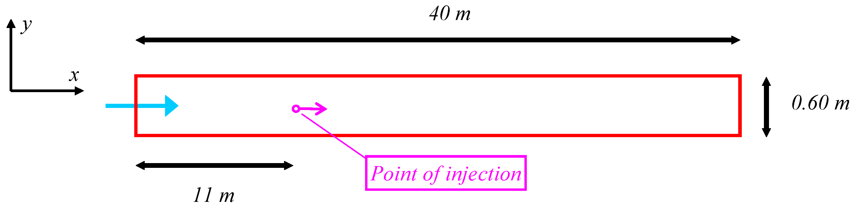
4.1. Contaminant Dispersion Due to Transverse Turbulent Mixing in a Shallow Water Flow
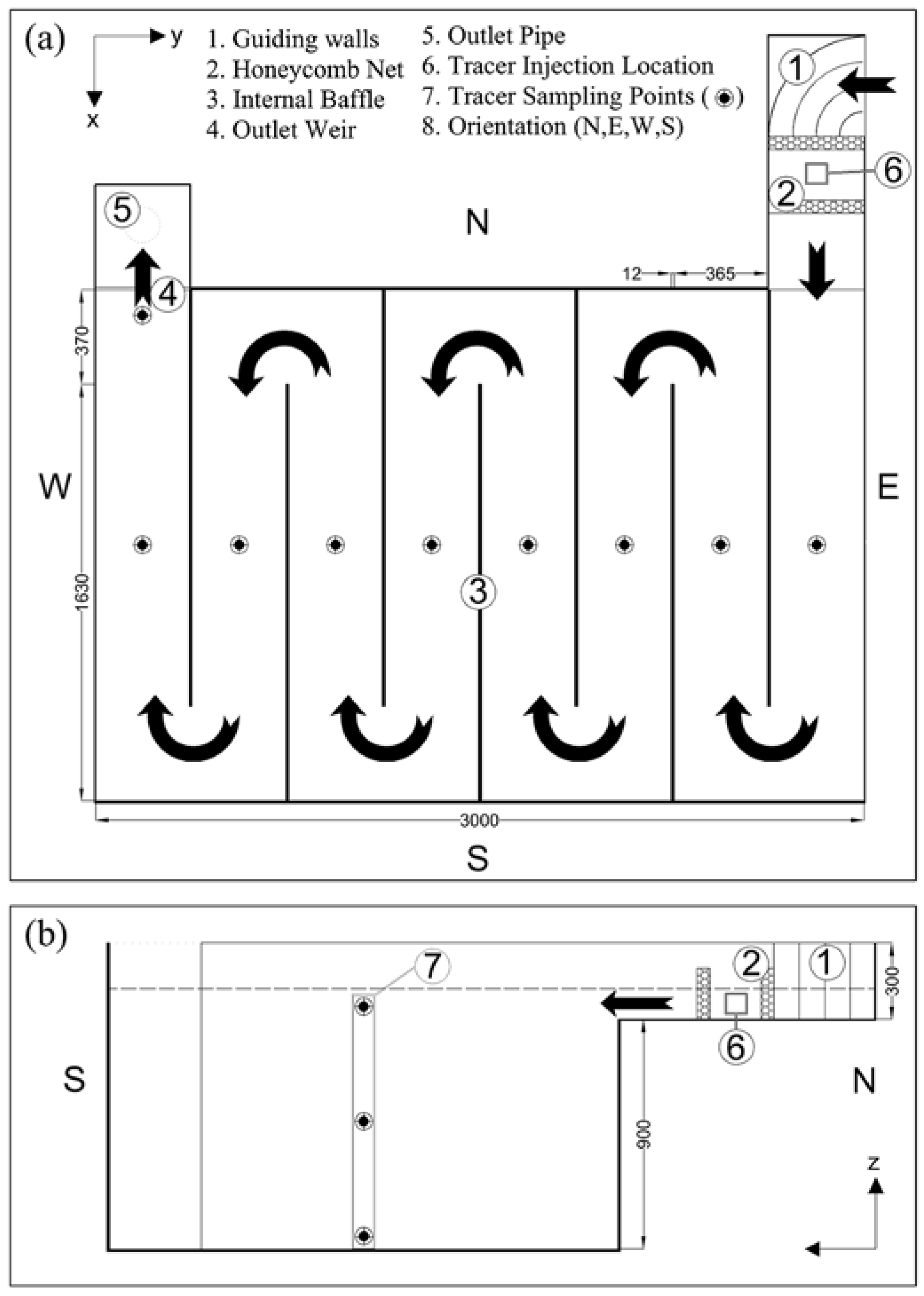
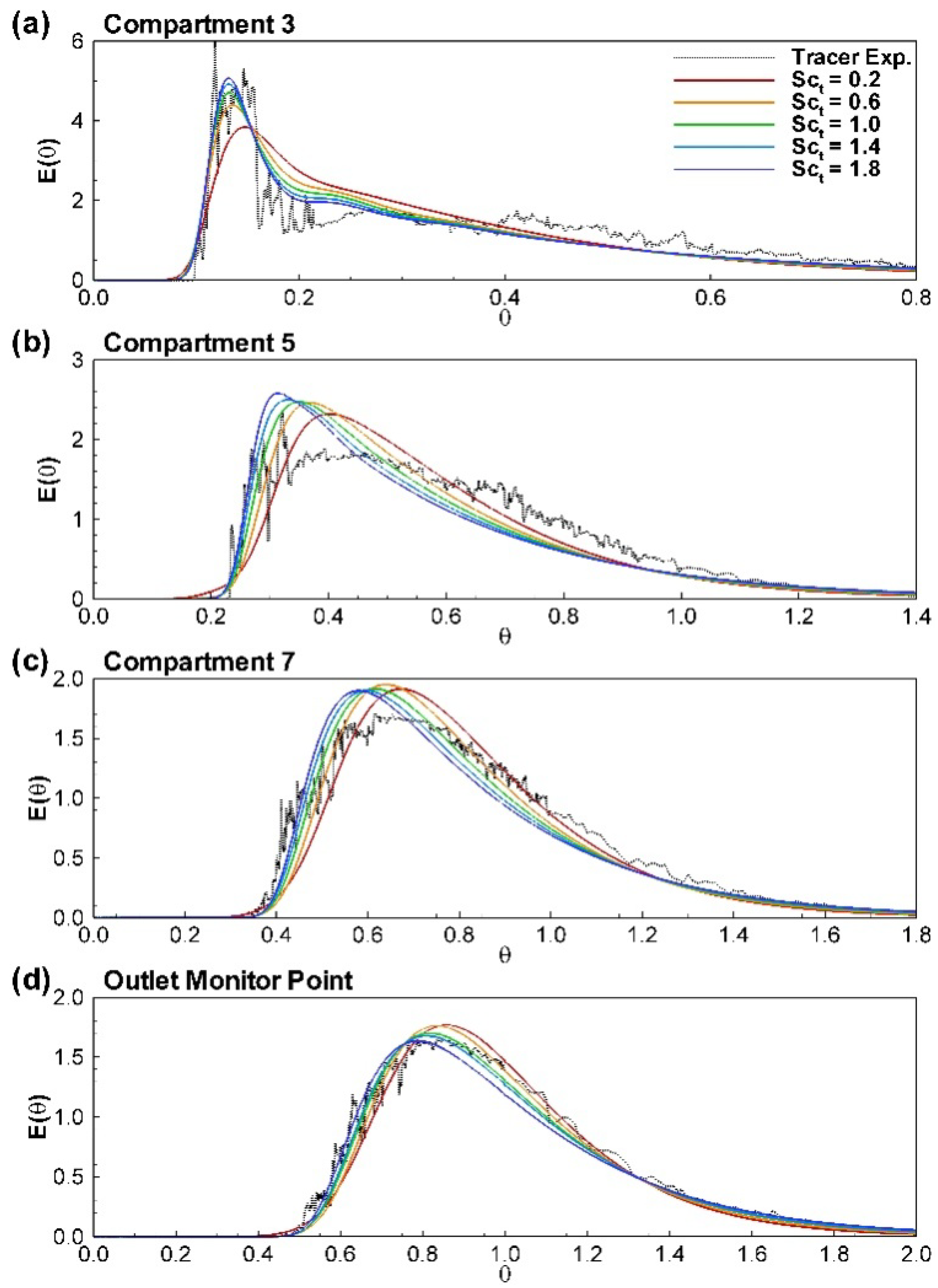
4.2. Tracer Transport in a Contact Tank
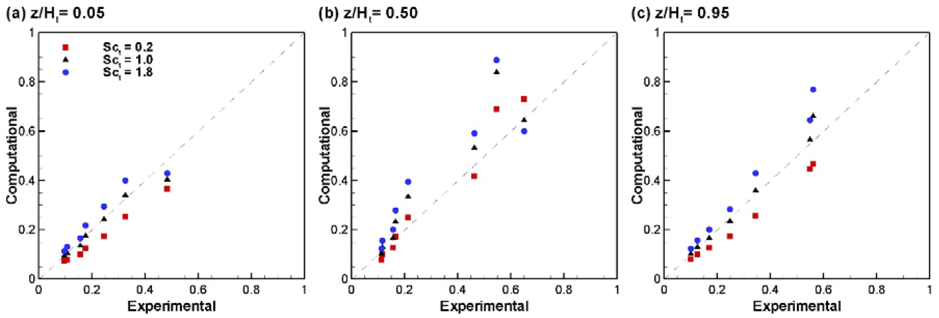
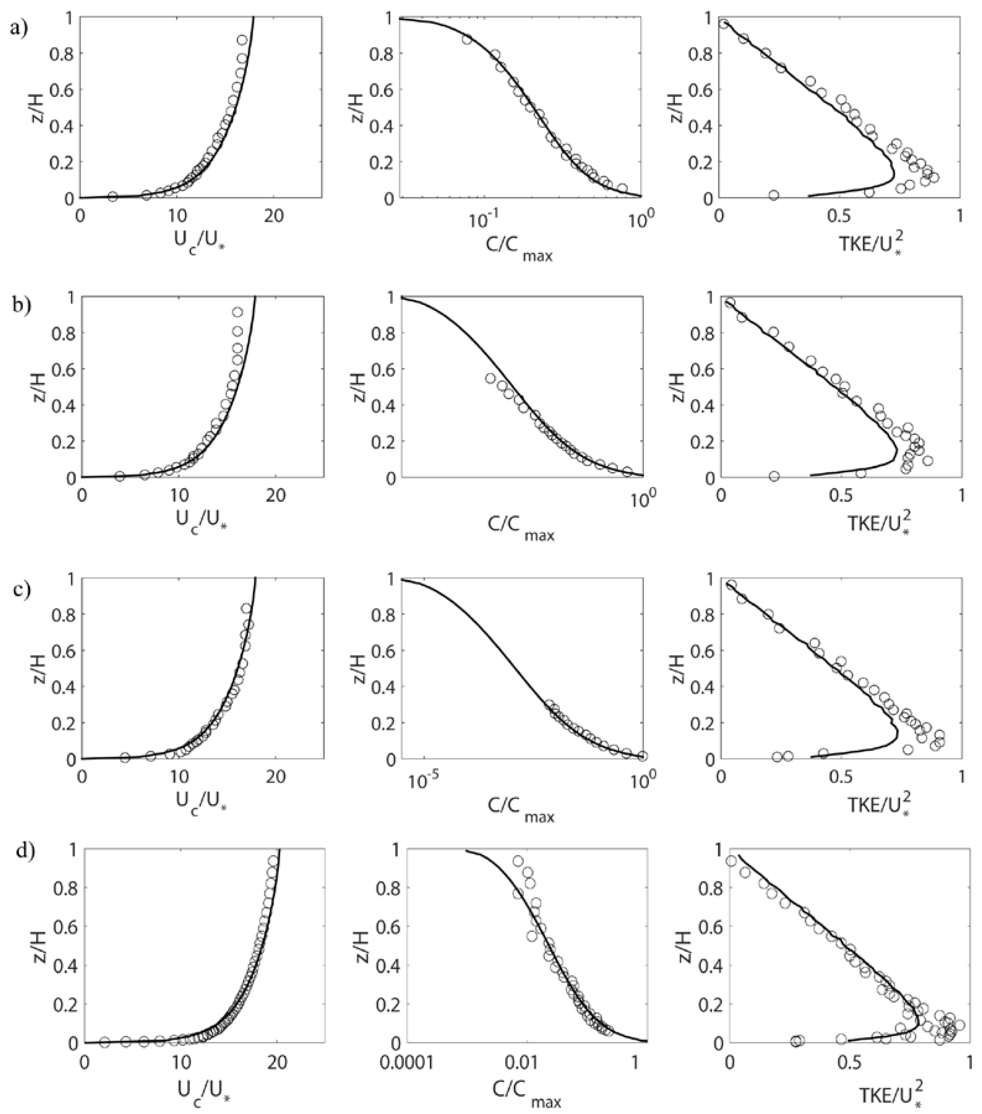
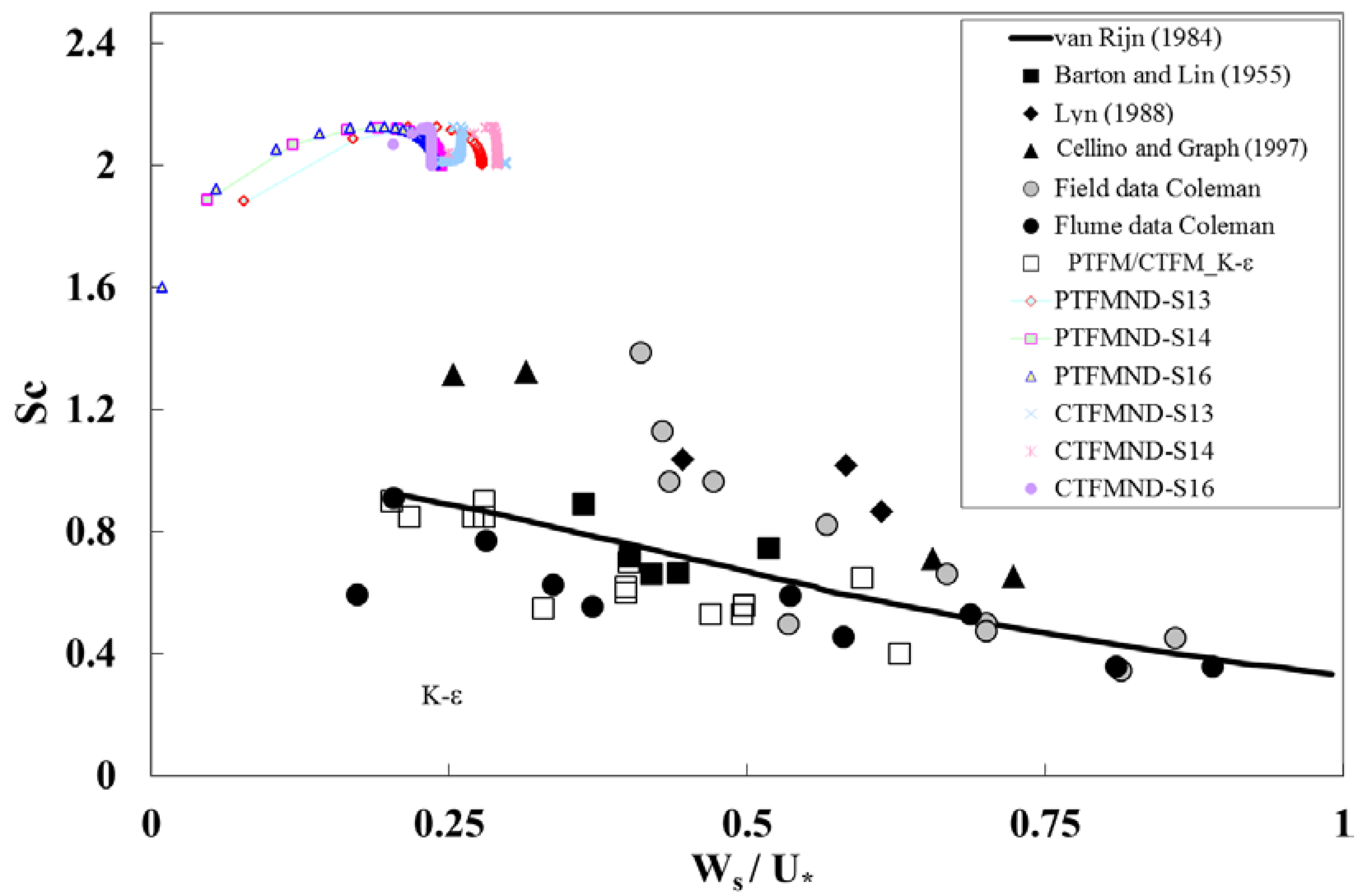
4.3. Sediment Transport in Suspension
5. Discussion
6. Conclusions
Acknowledgments
Author Contributions
Conflicts of Interest
References
- Cushman-Roisin, B.; Gualtieri, C.; Mihailovic, D.T. Environmental Fluid Mechanics: Current issues and future outlook. In Fluid Mechanics of Environmental Interfaces, 2nd ed.; Gualtieri, C., Mihailovic, D.T., Eds.; CRC Press/Balkema: Leiden, The Netherlands, 2012. [Google Scholar]
- Blocken, B.; Gualtieri, C. Ten iterative steps for model development and evaluation applied to Computational Fluid Dynamics for Environmental Fluid Mechanics. Environ. Model. Softw. 2012, 33, 1–22. [Google Scholar] [CrossRef]
- Jakeman, A.J.; Letcher, R.A.; Norton, J.P. Ten iterative steps in development and evaluation of environmental models. Environ. Model. Softw. 2006, 21, 602–614. [Google Scholar] [CrossRef]
- Zamani, K.; Bombardelli, F.A. Analytical solutions of nonlinear and variable-parameter transport equations for verification of numerical solvers. Environ. Fluid Mech. 2014, 14, 711–742. [Google Scholar] [CrossRef]
- The American Society of Mechanical Engineers (ASME). Standard for Verification and Validation in Computational Fluid Dynamics and Heat Transfer; ASME V & V 2009; The American Society of Mechanical Engineers (ASME): New York, NY, USA, 2009. [Google Scholar]
- Ercoftac. Best Practices Guidelines for Industrial Computational Fluid Dynamics. Version 1.0. Available online: http://www.ercoftac.org/ (accessed on 19 April 2017).
- Franke, J.; Hellsten, A.; Schlünzen, H.; Carissimo, B. Best practice guideline for the CFD simulation of flows in the urban environment. In COST 732: Quality Assurance and Improvement of Microscale Meteorological Models; COST Office Brussels: Bruxelles, Belgium, 2007. [Google Scholar]
- Ingham, D.B.; Ma, L. Fundamental equations for CFD river flow simulations. In Computational Fluid Dynamics. Applications in Environmental Hydraulics; Bates, P.D., Lane, S.N., Ferguson, R.I., Eds.; John Wiley & Sons: Chichester, UK, 2005; p. 534. [Google Scholar]
- Knight, D.W.; Wright, N.G.; Morvan, H.P. Guidelines for Applying Commercial CFD Software to Open Channel Flow. Report Based on Research Work Conducted under EPSRC Grants GR/R43716/01 and GR/R43723/01. 2005, p. 31. Available online: http://www.nottingham.ac.uk/cfd/ocf/Methodology.pdf (accessed on 18 April 2017).
- Tominaga, Y.; Mochida, A.; Yoshie, R.; Kataoka, H.; Nozu, T.; Yoshikawa, M.; Shirasawa, T. AIJ guidelines for practical applications of CFD to pedestrian wind environment around buildings. J. Wind Eng. Ind. Aerodyn. 2008, 96, 1749–1761. [Google Scholar] [CrossRef]
- Pope, S.B. Turbulent Flows; Cambridge University Press: Cambridge, UK, 2000; p. 806. [Google Scholar]
- Rossi, R.; Iaccarino, G. Numerical simulation of scalar dispersion downstream of a square obstacle using gradient-transport type models. Atmos. Environ. 2009, 43, 2518–2531. [Google Scholar] [CrossRef]
- Daly, B.J.; Harlow, F.H. Transport equations in turbulence. Phys. Fluids 1970, 13, 2634–2649. [Google Scholar] [CrossRef]
- Abe, K.; Suga, K. Towards the development of a Reynolds–Averaged algebraic turbulent scalar flux model. Int. J. Heat Fluid Flow 2001, 22, 19–29. [Google Scholar] [CrossRef]
- Fischer, H.B.; List, E.J.; Koh, R.C.Y.; Imberger, J.; Brook, N.H. Mixing in Inland and Coastal Waters; Academic Press: New York, NY, USA, 1979; p. 484. [Google Scholar]
- Cushman-Roisin, B. Beyond turbulent diffusivity. Environ. Fluid Mech. 2008, 8, 543–549. [Google Scholar] [CrossRef]
- Kim, D.; Stoesser, T.; Kim, J.H. The effect of baffle spacing on hydrodynamics and solute transport in serpentine contact tanks. J. Hydraul. Res. 2013, 51, 558–568. [Google Scholar] [CrossRef]
- Kim, D.; Stoesser, T.; Kim, J.H. Modeling aspects of flow and solute transport simulations in water disinfection tanks. Appl. Math. Model. 2013, 37, 8039–8050. [Google Scholar] [CrossRef]
- Kundu, P.K.; Cohen, I.M.; Dowling, D.R. Fluid Mechanics, 5th ed.; Elsevier Academic Press: San Diego, CA, USA, 2012; p. 892. [Google Scholar]
- Rodi, W. Turbulence Models and Their Application in Hydraulics—A State of the Art Review; International Association for Hydraulics Research: Delft, The Netherlands, 1980. [Google Scholar]
- Hanjalić, K. Closure Models for Incompressible Turbulent Flows; Lecture Notes; Von Kármán Institute: Sint-Genesius-Rode, Belgium, 2004; p. 75. [Google Scholar]
- Arnold, U.; Hottges, J.; Rouv, G. Turbulence and mixing mechanisms in compound open channel flow. In Proceedings of the 23th IAHR Congress, Ottawa, ON, Canada, 21–25 August 1989. [Google Scholar]
- Djordjevic, S. Mathematical model of unsteady transport and its experimental verification in a compound open channel flow. J. Hydraul. Res. 1993, 31, 229–248. [Google Scholar] [CrossRef]
- Lin, B.; Shiono, K. Numerical modelling of solute transport in compound channel flows. J. Hydraul. Res. 1995, 33, 773–788. [Google Scholar] [CrossRef]
- Simões, F.J.M.; Wang, S.S.Y. Numerical prediction of three dimensional mixing in a compound channel. J. Hydraul. Res. 1997, 35, 619–642. [Google Scholar] [CrossRef]
- Angeloudis, A.; Stoesser, T.; Gualtieri, C.; Falconer, R.A. Contact Tank Design Impact on Process Performance. Environ. Model. Assess. 2016, 21, 563–576. [Google Scholar] [CrossRef]
- Angeloudis, A.; Stoesser, T.; Kim, D.; Falconer, R.A. Modelling of flow, transport and disinfection kinetics in contact tanks. Proc. Inst. Civ. Eng. Water Manag. 2014, 167, 532–546. [Google Scholar] [CrossRef]
- Angeloudis, A.; Stoesser, T.; Falconer, R.A. Predicting the disinfection efficiency range in chlorine contact tanks through a CFD-based approach. Water Res. 2014, 60, 118–129. [Google Scholar] [CrossRef] [PubMed]
- Angeloudis, A.; Stoesser, T.; Falconer, R.A.; Kim, D. Flow, transport and disinfection performance in small- and full-scale contact tanks. J. Hydro Environ. Res. 2015, 9, 15–27. [Google Scholar] [CrossRef]
- Gualtieri, C. Numerical simulation of flow and tracer transport in a disinfection contact tank. In Proceedings of the 3rd Biennial Meeting of the International Environmental Modelling and Software Society, Burlington, VT, USA, 9–12 July 2006. [Google Scholar]
- Kim, D.; Kim, D.; Kim, J.H.; Stoesser, T. Large Eddy Simulation of flow and tracer transport in multichamber ozone contactors. J. Environ. Eng. 2010, 136, 22–31. [Google Scholar] [CrossRef]
- Martínez-Solano, F.J.; Iglesias-Rey, P.L.; Gualtieri, C.; López-Jiménez, P.A. Modelling flow and concentration field in a 3D rectangular water tank. In Proceedings of the 5th Biennial Meeting of the International Environmental Modelling and Software Society, Ottawa, ON, Canada, 5–8 July 2010; Volume I, pp. 389–398. [Google Scholar]
- Rauen, B.; Angeloudis, A.; Falconer, R.A. Appraisal of chlorine contact tank modelling practices. Water Res. 2012, 46, 5834–5847. [Google Scholar] [CrossRef] [PubMed]
- Zhang, J.; Tejada-Martinez, A.E.; Zhang, Q. Developments in computational fluid dynamics-based modeling for disinfection technologies over the last two decades: A review. Environ. Model. Softw. 2014, 58, 71–85. [Google Scholar] [CrossRef]
- Zhang, J.; Tejada-Martinez, A.E.; Zhang, Q. Evaluation of Large Eddy Simulation and RANS for determining hydraulic performance of disinfection systems for water treatment. J. Fluids Eng. 2014, 136, 121102. [Google Scholar] [CrossRef]
- Zhang, J.; Tejada-Martinez, A.E.; Zhang, Q. Rapid analysis of disinfection efficiency through computational fluid dynamics. J. Am. Water Works Assoc. 2016, 108, E50–E59. [Google Scholar] [CrossRef]
- Oliver, C.J.; Davidson, M.J.; Nokes, R.I. k–ε Predictions of the initial mixing of desalination discharges. Environ. Fluid Mech. 2008, 8, 617–625. [Google Scholar] [CrossRef]
- Absi, R. Concentration profiles for fine and coarse sediments suspended by waves over ripples: An analytical study with the 1-DV gradient diffusion model. Adv. Water Resour. 2010, 33, 411–418. [Google Scholar] [CrossRef]
- Amoudry, L.; Hsu, T.-J.; Liu, P.L. Schmidt number and near-bed boundary condition effects on a two-phase dilute sediment transport model. J. Geophys. Res. 2005, 110, C09003. [Google Scholar] [CrossRef]
- Bombardelli, F.A.; Jha, S.K. Hierarchical modeling of the dilute transport of suspended sediment in open channels. Environ. Fluid Mech. 2009, 9, 207–235. [Google Scholar] [CrossRef]
- Graf, W.H.; Cellino, M. Suspension flow in open channels; experimental study. J. Hydraul. Res. 2002, 15, 435–447. [Google Scholar] [CrossRef]
- Hsu, T.-J.; Liu, P.L.-F. Toward modeling turbulent suspension of sand in the nearshore. J. Geophys. Res. 2004, 109, C06018. [Google Scholar] [CrossRef]
- Jha, S.K. Effect of particle inertia on the transport of particle-laden open channel flow. Eur. J. Mech. B Fluids 2017, 62, 32–41. [Google Scholar] [CrossRef]
- Jha, S.K.; Bombardelli, F.A. Two-phase modeling of turbulence in dilute sediment-laden, open-channel flows. Environ. Fluid Mech. 2009, 9, 237–266. [Google Scholar] [CrossRef]
- Jha, S.K.; Bombardelli, F.A. Toward two-phase flow modeling of nondilute sediment transport in open channels. J. Geophys. Res. Earth Surf. 2010, 115, F03015. [Google Scholar] [CrossRef]
- Jha, S.K.; Bombardelli, F.A. Theoretical/numerical model for the transport of non-uniform suspended sediment in open channels. Adv. Water Resour. 2011, 34, 577–591. [Google Scholar] [CrossRef]
- Muste, M.; Patel, V. Velocity profiles for particles and liquid in open-channel flow with suspended sediment. J. Hydraul. Eng. 1997, 123, 742–751. [Google Scholar] [CrossRef]
- Muste, M.; Yu, K.; Fujita, I.; Ettema, R. Two-phase versus mixed-flow perspective on suspended sediment transport in turbulent channel flows. Water Resour. Res. 2005, 41, W10402. [Google Scholar] [CrossRef]
- Huang, H.; Imran, J.; Pirmez, C. Numerical model of turbidity currents with a deforming bottom boundary. J. Hydraul. Eng. 2005, 131, 283–293. [Google Scholar] [CrossRef]
- Huq, P.; Stewart, E.J. Measurements and analysis of the turbulent Schmidt number in density stratified turbulence. Geophys. Res. Lett. 2008, 35, L23604. [Google Scholar] [CrossRef]
- Walker, C.; Manera, A.; Niceno, B.; Simiano, M.; Prasser, H.-M. Steady-state RANS–simulations of the mixing in a T–junction. Nucl. Eng. Des. 2010, 240, 2107–2115. [Google Scholar] [CrossRef]
- Toorman, E.A. Vertical mixing in the fully developed turbulent layer of sediment-laden open-channel flow. J. Hydraul. Eng. 2008, 134, 1225–1235. [Google Scholar] [CrossRef]
- Salzano, F.; Gualtieri, C. The effect of baffle spacing on hydrodynamics and solute transport in serpentine contact tanks. J. Hydraul. Res. 2014, 52, 152–154. [Google Scholar] [CrossRef][Green Version]
- Mokhtarzadeh-Dehghan, M.R.; Akcayoglu, A.; Robins, A.G. Numerical study and comparison with experiment of dispersion of a heavier-than-air gas in a simulated neutral atmospheric boundary layer. J. Wind Eng. Ind. Aerodyn. 2012, 110, 10–24. [Google Scholar] [CrossRef]
- Van Rijn, L.C. Sediment transport, part II: Suspended load transport. J. Hydraul. Eng. 1984, 110, 1613–1641. [Google Scholar] [CrossRef]
- Ribberink, J.S.; Al-Salem, A.A. Sheet flow and suspension of sand in oscillatory boundary layers. Coast. Eng. 1995, 25, 205–225. [Google Scholar] [CrossRef]
- Cellino, M. Suspension Flow in Open Channel. Ph.D. Thesis, Ecole Polytechnique federale de Lausanne, Lausanne, Switzerland, 1998. [Google Scholar]
- Blocken, B.; Stathopoulos, T.; Saathoff, P.; Wang, X. Numerical evaluation of pollutant dispersion in the built environment: Comparisons between models and experiments. J. Wind Eng. Ind. Aerodyn. 2008, 96, 1817–1831. [Google Scholar] [CrossRef]
- Chavez, M.; Hajra, B.; Stathopoulos, T.; Bahloul, A. Near-field pollutant dispersion in the built environment by CFD and wind tunnel simulations. J. Wind Eng. Ind. Aerodyn. 2011, 99, 330–339. [Google Scholar] [CrossRef]
- Chen, B.; Liu, S.; Miao, Y.; Wang, S.; Li, Y. Construction and validation of an urban area flow and dispersion model on building scales. Acta Meteorol. Sin. 2014, 27, 923–941. [Google Scholar] [CrossRef]
- Di Sabatino, S.; Buccolieri, S. MUST experiment simulations using CFD and integral models. In Proceedings of the 11th International Conference on Harmonisation within Atmospheric Dispersion Modelling for Regulatory Purpose, Cambridge, UK, 2–5 July 2007. [Google Scholar]
- Ebrahimi, M.; Jahangirian, A. New analytical formulations for calculation of dispersion parameters of Gaussian model using parallel CFD. Environ. Fluid Mech. 2013, 13, 125–144. [Google Scholar] [CrossRef]
- Flesch, T.K.; Prueger, J.H.; Hatfield, J.L. Turbulent Schmidt number from a tracer experiment. Agric. For. Meteorol. 2002, 111, 299–307. [Google Scholar] [CrossRef]
- Galeazzo Cunha, F.C.; Donnert, G.; Cárdenas, C.; Sedlmaier, J.; Habisreuther, P.; Zarzalis, N.; Beck, C.; Krebs, W. Computational modeling of turbulent mixing in a jet in crossflow. Int. J. Heat Fluid Flow 2013, 41, 55–65. [Google Scholar] [CrossRef]
- Hassan, E.; Aono, H.; Boles, J.; Douglas, D.; Shyy, W. Adaptive Turbulent Schmidt Number approach for multi-scale simulation of supersonic crossflow. In Proceedings of the 20th AIAA Computational Fluid Dynamics Conference, Honolulu, HI, USA, 27–30 June 2011. [Google Scholar]
- Koeltzsch, K. The height dependence of the turbulent Schmidt number within the boundary layer. Atmos. Environ. 2000, 34, 1147–1151. [Google Scholar] [CrossRef]
- Tominaga, Y.; Stathopoulos, T. Turbulent Schmidt numbers for CFD analysis with various types of flowfield. Atmos. Environ. 2007, 41, 8091–8099. [Google Scholar] [CrossRef]
- Riddle, A.; Carruthers, D.; Sharpe, A.; McHugh, C.; Stocker, J. Comparisons between FLUENT and ADMS for atmospheric dispersion modelling. Atmos. Environ. 2004, 38, 1029–1038. [Google Scholar] [CrossRef]
- Wilson, J.D. Turbulent Schmidt numbers above a wheat crop. Bound. Layer Meteorol. 2013, 148, 255–268. [Google Scholar] [CrossRef]
- Goldberg, U.; Palaniswamy, S.; Batten, P.; Gupta, V. Variable turbulent Schmidt and Prandtl number modeling. Eng. Appl. Comput. Fluid Mech. 2010, 4, 511–520. [Google Scholar] [CrossRef]
- Ross, A.N. Scalar transport over forested hills. Bound. Layer Meteorol. 2011, 141, 179–199. [Google Scholar] [CrossRef]
- Shi, Z.; Chen, J.; Chen, Q. On the turbulence models and turbulent Schmidt number in simulating stratified flows. J. Build. Perform. Simul. 2016, 9, 134–178. [Google Scholar] [CrossRef]
- Gualtieri, C. RANS–based simulation of transverse turbulent mixing in a 2D geometry. Environ. Fluid Mech. 2010, 10, 137–156. [Google Scholar] [CrossRef]
- Lau, Y.L.; Krishnappan, B.G. Transverse dispersion in rectangular channel. J. Hydraul. Div. 1977, 103, 1173–1189. [Google Scholar]
- Van Prooijen, B.C.; Uijttewaal, W.S.J. Horizontal mixing in shallow flows. In Water Quality Hazards and Dispersion of Pollutants; Czernuszenko, W., Rowinski, P., Eds.; Springer Science + Business Inc.: New York, NY, USA, 2005; p. 250. [Google Scholar]
- Rutherford, J.C. River Mixing; John Wiley & Sons: Chichester, UK, 1994; p. 348. [Google Scholar]
- Rummel, A.C.; Socolofsky, S.A.; v.Carmer, C.F.; Jirka, G.H. Enhanced diffusion from a continuous point source in shallow free-surface flow with grid turbulence. Phys. Fluids 2005, 17, 075105-1–075105-12. [Google Scholar] [CrossRef]
- Stamou, A.I. Improving the hydraulic efficiency of water process tanks using CFD models. Chem. Eng. Process. Process Intensif. 2008, 47, 1179–1189. [Google Scholar] [CrossRef]
- Teixeira, E.C.; Siqueira, R.N. Performance assessment of hydraulic efficiency indexes. J. Environ. Eng. 2008, 134, 851–859. [Google Scholar] [CrossRef]
- Launder, B.E. Heat and Mass Transport. In Turbulence; Bradshaw, P., Ed.; Springer: Berlin, Germany, 1978. [Google Scholar]
- Markse, D.M.; Boyle, J.D. Chlorine contact chamber design—A field evaluation. Water Sew. Works 1978, 120, 70–77. [Google Scholar]
- Rouse, H. Modern conceptions of the mechanics or fluid turbulence. Trans. Am. Soc. Civ. Eng. 1937, 102, 463–505. [Google Scholar]
- Vanoni, V.A. Transportation of suspended sediment by water. Trans. Am. Soc. Civ. Eng. 1946, 111, 67–102. [Google Scholar]
- Garcia, M. Sedimentation Engineering: Processes, Measurements, Modeling, and Practice; ASCE (American Society of Civil Engineers): New York, NY, USA, 2008. [Google Scholar]
- Parker, G. 1D Sediment Transport Morphodynamics with Applications to Rivers and Turbidity Currents; St. Anthony Falls Laboratory, University of Minnesota: Minneapolis, MN, USA, 2004. [Google Scholar]
- Hunt, J. The turbulent transport of suspended sediment in open channels. Proc. R. Soc. Lond. A Math. Phys. Eng. Sci. 1954, 224, 322–335. [Google Scholar] [CrossRef]
- Greimann, B.; Muste, M.; Holly, F., Jr. Two-phase formulation of suspended sediment transport. J. Hydraul. Res. 1999, 37, 479–500. [Google Scholar] [CrossRef]
- Bombardelli, F.A. Turbulence in Multiphase Models for Aeration Bubble Plumes. Ph.D. Thesis, University of Illinois Urbana-Champaign, Champaign, IL, USA, 2004. [Google Scholar]
- Bombardelli, F.A.; Bizier, P.; DeBarry, P. Characterization of coherent structures from parallel, LES computations of wandering effects in bubble plumes. Bridges 2003, 10, 159. [Google Scholar]
- Buscaglia, G.C.; Bombardelli, F.A.; Garcı́a, M.H. Numerical modeling of large-scale bubble plumes accounting for mass transfer effects. Int. J. Multiph. Flow 2002, 28, 1763–1785. [Google Scholar] [CrossRef]
- Cellino, M.; Graf, W. Measurements on suspension flow in open channels. In Environmental and Coastal Hydraulics Protecting the Aquatic Habitat; American Society of Civil Engineers (ASCE): New York, NY, USA, 1997; pp. 179–184. [Google Scholar]
- Lyn, D. A similarity approach to turbulent sediment-laden flows in open channels. J. Fluid Mech. 1988, 193, 1–26. [Google Scholar] [CrossRef]
- Nezu, I.; Azuma, R. Turbulence characteristics and interaction between particles and fluid in particle-laden open channel flows. J. Hydraul. Eng. 2004, 130, 988–1001. [Google Scholar] [CrossRef]
- Barton, J.; Lin, P. A Study of the Sediment Transport in Alluvial Streams; Civil Engineering Department Report; Colorado Agricultural and Mechanical College, Department of Civil Engineering: Fort Collins, CO, USA, 1955. [Google Scholar]
- Coleman, N.L. Velocity profiles with suspended sediment. J. Hydraul. Res. 1981, 19, 211–229. [Google Scholar] [CrossRef]
- Einstein, H.; Chien, N. Effects of Heavy Sediment Concentration Near the Bed on Velocity and Sediment Distribution; University of California, Institute of Engineering Research: Berkeley, CA, USA, 1955. [Google Scholar]
- Combest, D.P.; Ramachandran, P.A.; Dudukovic, M.P. On the gradien diffusion hypothesis and passive scalar transport in turbulent flows. Ind. Eng. Chem. Res. 2011, 50, 8817–8823. [Google Scholar] [CrossRef]
- Reynolds, A. The prediction of turbulent Prandtl and Schmidt numbers. Int. J. Heat Mass Transf. 1975, 18, 1055–1069. [Google Scholar] [CrossRef]
- Dudukovic, A.; Pjanovic, R. Effect of Turbulent Schmidt Number on Mass-Transfer Rates to Falling Liquid Films. Ind. Eng. Chem. Res. 1999, 38, 2503–2504. [Google Scholar] [CrossRef]
- Donzis, D.A.; Konduri, A.; Sreenivasan, K.R.; Yeung, P.K. The turbulent Schmidt number. J. Fluids Eng. 2014, 136, 060912. [Google Scholar] [CrossRef]


| Substance | Formula | Schmidt Number Sc for T = 25 °C | |
|---|---|---|---|
| Air | Water | ||
| Methane | CH4 | 0.99 | 570 |
| Oxygen | O2 | 0.84 | 441 |
| Nitrogen | N2 | --- | 240 |
| Carbon dioxide | CO2 | 1.14 | 410 |
| Ammonia | NH3 | 0.57 | 360 |
| Ethanol | C2H6O | 1.50 | 540 |
| Methanol | CH3OH | 1.14 | 540 |
| Cyclohexane | C6H12 | --- | 985 |
| Reference | Environmental Flow | Comments |
|---|---|---|
| Arnold et al. [22] | Flow and tracer transport in open channels | Exp − Sct = 0.5–0.9 |
| Djordjevic [23] | Flow and tracer transport in open channels | Exp/Num − Sct = 1 |
| Lin and Shiono [24] | Flow and tracer transport in open channels | Exp/Num − Sct = 0.72 |
| Simões and Wang [25] | Flow and tracer transport in open channels | Exp/Num − Sct = 0.5 (horizontal), 1 (vertical) |
| Gualtieri [30] | Flow and tracer transport in a contact tank | Exp/Num − Sct = 1 |
| Rauen et al. [33] | Flow and tracer transport in a contact tank | Exp/Num − Sct = 1 |
| Kim et al. [31] | Flow and tracer transport in a contact tank | Exp/Num − Sct = 0.3 |
| Zhang et al. [34,35,36] | Flow and tracer transport in a contact tank | Exp/Num − Sct = 0.7 |
| Angeloudis et al. [26,27,28,29] | Flow and tracer transport in a contact tank | Exp/Num − Sct = 0.7 |
| Martínez-Solano et al. [32] | Flow and tracer transport in a water tank | Exp/Num − Sct = 0.7 |
| Oliver et al. [37] | Inclined negatively buoyant discharges | Exp/Num − Sct = 0.6 |
| Graf and Cellino [41] | Sediment-laden open channel flows | Exp − Sct > 1 (no bedforms), Sct < 1 (bedforms) |
| Hsu and Liu [42] | Sediment-laden open channel flows | Exp/Num − Sct = 0.7 |
| Amoudry et al. [39] | Sediment-laden open channel flows | Exp/Num − Sct = 0.7 (bed), Sct = 0.52 (surface) |
| Muste et al. [47,48] | Sediment-laden open channel flows | Exp − Sct = 1. 4–2.11 (sand), Sct = 0.22–0.52 (nylon) |
| Toorman [52] | Sediment-laden open channel flows | Exp/Num − Sct = 0.5–0.8 |
| Bombardelli and Jha [40] | Sediment-laden open channel flows | Exp/Num − Sct = 0.56–0.7 (dilute mixtures) |
| Jha and Bombardelli [44,45,46] | Sediment-laden open channel flows | Exp/Num − Sct = 0.4–0.9 (k-ε model) |
| Jha [43] | Sediment-laden open channel flows | Exp/Num − Sct = 0.2–1.3 |
| Absi [38] | Sediment-laden open channel flows | Exp/Num − Sct = Sct (z) |
| Huang et al. [49] | Density stratified turbulence | Exp/Num − Sct = 1.3 |
| Huq and Stewart [50] | Density stratified turbulence | Exp − Sct = Sct (Ri, T*) |
| Walker et al. [51] | T-junction mixing experiments | Exp/Num − Sct = 0.1–0.2 |
| Reference | Environmental Flow | Comments |
|---|---|---|
| Koeltzsch [66] | Tracer transport in a boundary layer | Exp − Sct = 0.3–1, Sct = Sct (BL height) |
| Flesch et al. [63] | Contaminant emission from soil | Exp − Sct = 0.6 |
| Wilson [69] | Concentration measurements above a wheat crop | Exp − Sct = 0.68 and 0.78 |
| Tominaga and Stathopoulos [67] | Review paper | Exp/Num − Sct = 0.2–1.3 |
| Riddle et al. [68] | Pollutant dispersion in the built environment | Exp/Num − Sct = 0.3 and 0.7 |
| Di Sabatino and Buccolieri [61] | Pollutant dispersion in the built environment | Exp/Num − Sct = 0.4 and 0.7 |
| Blocken et al. [58] | Pollutant dispersion in the built environment | Exp/Num − Sct = 0.3–1 |
| Chavez et al. [59] | Pollutant dispersion in the built environment | Exp/Num − Sct = 0.1–0.7 |
| Mokhtarzadeh-Dehghan et al. [54] | Pollutant dispersion in the built environment | Exp/Num − Sct = 0.4–2.5 as f(Ri*) |
| Ebrahimi and Jahangirian [62] | Pollutant dispersion in the built environment | Exp/Num − Sct = 0.7 |
| Chen et al. [60] | Pollutant dispersion in the built environment | Exp/Num − Sct = 1.0 and corrected from wind tunnel data |
| Hassan et al. [65] | Supersonic crossflow | Exp/Num − Sct = 1.0 and adaptive Sct |
| Galeazzo et al. [64] | Jet in crossflow | Exp/Num − Sct = 0.3–0.9 |
| Goldberg et al. [70] | Different type of air flows | Exp/Num − Sct variable |
| Ross [71] | Flow over forested hills | Exp/Num − Sct = Sct (z) |
| Shi et al. [72] | Density stratified jets | Exp/Num − Sct = Sct (velocity and density gradient) |
| Run | Sct | Dt-y (m2/s) | Reference |
|---|---|---|---|
| Exp. | --- | 1.41 × 10⁻⁴ | Lau and Krishnappan [74] |
| 1 | 0.8 | 2.10 × 10⁻⁴ | Present study |
| 2 | 0.9 | 1.95 × 10⁻⁴ | Present study |
| 3 | 1.0 | 1.88 × 10⁻⁴ | Gualtieri [73] |
| 4 | 1.2 | 1.51 × 10⁻⁴ | Present study |
| 5 | 1.3 | 1.42 × 10⁻⁴ | Present study |
| Numerical Model Sct | Outlet Hydraulic Efficiency Indicators | |||||
|---|---|---|---|---|---|---|
| tp/T | t10/T | t90/T | tg/T | Μο | σ2 | |
| 0.2 | 0.904 | 0.702 | 1.345 | 0.991 | 1.933 | 0.074 |
| 0.4 | 0.843 | 0.700 | 1.356 | 0.994 | 1.938 | 0.077 |
| 0.6 | 0.834 | 0.695 | 1.374 | 0.998 | 1.976 | 0.082 |
| 0.8 | 0.825 | 0.690 | 1.391 | 1.001 | 2.015 | 0.088 |
| 1.0 | 0.817 | 0.685 | 1.407 | 1.004 | 2.052 | 0.093 |
| 1.2 | 0.809 | 0.681 | 1.421 | 1.006 | 2.087 | 0.099 |
| 1.4 | 0.802 | 0.677 | 1.435 | 1.009 | 2.120 | 0.104 |
| 1.6 | 0.794 | 0.674 | 1.448 | 1.011 | 2.150 | 0.108 |
| 1.8 | 0.788 | 0.671 | 1.460 | 1.013 | 2.177 | 0.113 |
| Exp. | 0.833 | 0.695 | 1.418 | 1.005 | 2.113 | 0.097 |
| Authors | Technique for Velocity Measurements | Variables Observed * |
|---|---|---|
| Lyn [92] | Laser-Doppler anemometry | Vmix, C |
| Muste and Patel [47] | Discriminator laser-Doppler velocimetry | Vc, Vd, T |
| Nezu and Azuma [93] | Particle tracking velocimetry | Vc, Vd, C, T |
| Muste et al. [48] | Particle image velocimetry and particle tracking velocimetry | Vc, Vd, C, T |
© 2017 by the authors. Licensee MDPI, Basel, Switzerland. This article is an open access article distributed under the terms and conditions of the Creative Commons Attribution (CC BY) license (http://creativecommons.org/licenses/by/4.0/).
Share and Cite
Gualtieri, C.; Angeloudis, A.; Bombardelli, F.; Jha, S.; Stoesser, T. On the Values for the Turbulent Schmidt Number in Environmental Flows. Fluids 2017, 2, 17. https://doi.org/10.3390/fluids2020017
Gualtieri C, Angeloudis A, Bombardelli F, Jha S, Stoesser T. On the Values for the Turbulent Schmidt Number in Environmental Flows. Fluids. 2017; 2(2):17. https://doi.org/10.3390/fluids2020017
Chicago/Turabian StyleGualtieri, Carlo, Athanasios Angeloudis, Fabian Bombardelli, Sanjeev Jha, and Thorsten Stoesser. 2017. "On the Values for the Turbulent Schmidt Number in Environmental Flows" Fluids 2, no. 2: 17. https://doi.org/10.3390/fluids2020017
APA StyleGualtieri, C., Angeloudis, A., Bombardelli, F., Jha, S., & Stoesser, T. (2017). On the Values for the Turbulent Schmidt Number in Environmental Flows. Fluids, 2(2), 17. https://doi.org/10.3390/fluids2020017