Advancing CFD Simulations Through Machine-Learning-Enabled Mesh Refinement Analysis

Abstract

As computational fluid dynamics (CFD) has become more mainstream in production engineering workflows, new demands have been introduced that require high-quality meshes to accurately capture the complex geometries. This evolution has created the need for mesh generation frameworks that help engineers design optimized meshing structures for each new geometry. However, many simulation workflows rely on the experience and intuition of senior engineers rather than systematic frameworks. In this paper, a novel technique for determining mesh convergence is created using machine learning (ML). This method seeks to provide process engineers with a visual feedback mechanism of flow regions that require mesh refinement. The work was accomplished by creating three grid sensitivity studies on various geometries: zero-pressure-gradient flat plate, bump in channel, and axisymmetric free jet. The cases were then simulated using the Reynolds Averaged Navier-Stokes (RANS) models in OpenFOAM (v2306) and had the ML method applied post-hoc using Python (v3.12.6). To apply the method to each case, the flow field was regionalized and clustered using an unsupervised ML model. The ML clustering results were then converted into a similarity score, which compares two grid levels to inform the user whether the region of the flow had converged. To prove this framework, the similarity scores were compared to flow field probes used to determine mesh convergence at key points in the flow. The method was found to be in agreement with the flow field probes on the level of mesh refinement that created convergence. The approach was also seen to provide refinement region recommendations in regions of the flow that align with human intuition of the physics of the flow.

1. Introduction

Over the past three decades, advances in computing power and cost efficiency have dramatically expanded the use of computational fluid dynamics (CFD) in engineering design and analysis workflows. Scale-resolved methods such as Detached Eddy Simulation (DES) [1], once considered prohibitively expensive for high-fidelity high-Reynolds number external aerodynamic simulations, are now routinely employed in both automotive and aerospace engineering [2,3]. As CFD has become a mainstream tool in production workflows, its growing capabilities have introduced new demands, particularly the need for large, high-quality meshes that would accurately capture complex geometries and fully exploit the capabilities of high-fidelity simulation models. This evolution has created a pressing need for systematic frameworks that enable engineers to design complex workflows and generate simulations with optimized mesh structures and parameters tailored to each digital geometry. Despite this need, many simulation practices remain heuristic, relying on the experience and intuition of senior engineers rather than well-defined guidelines. Mesh generation is a prime example: although it has a decisive influence on simulation accuracy and stability, concrete, universally accepted rules for mesh design and quality assurance remain scarce. This gap persists even amid notable progress in higher-order meshing techniques [4,5,6] and automated tools such as adaptive mesh refinement (AMR) [7,8]. Yet, tools that provide direct feedback on the effectiveness of a chosen meshing strategy remain limited, underscoring the need for more systematic, data-driven approaches to mesh evaluation and refinement.

Capturing complex flow fields in CFD simulations still largely relies on the engineer’s experience and intuition. Refinement regions and meshing rules are typically defined manually around the geometry, with the expectation rather than assurance that these choices will improve solution fidelity. To assess whether a solution is independent of mesh resolution, engineers commonly perform a mesh sensitivity study in which a sequence of globally refined meshes, within computing restraints, is generated. The solutions obtained from these meshes are compared to identify the point at which further refinement produces negligible changes, indicating mesh convergence. For external aerodynamic flows, this convergence is generally evaluated by monitoring macro-level flow quantities such as lift, skin friction, or scalar field distributions, including velocity or pressure at selected locations. More formalized approaches, including Richardson extrapolation [9] and the Grid Convergence Index (GCI) [10,11,12,13,14], are well established in the literature. The GCI method was further refined by Eça and Hoekstra [15,16], who introduced an enhanced framework for uncertainty quantification in grid convergence studies. However, all these methods share a fundamental limitation: they can only indicate whether certain integral or local quantities have become mesh independent; they do not reveal which specific regions of the mesh are responsible for residual errors or sensitivity. To address this, Inthavong et al. [17] proposed a visualization-based approach, mapping two-dimensional slices of the solution fields from different meshes onto a common uniform grid and comparing the resulting differences. While this method provides qualitative insight into local flow discrepancies between meshes, it lacks a systematic mechanism to evaluate multiple flow features simultaneously. Consequently, users must manually interpret several different fields to judge whether the overall solution has reached grid independence. In practice, this leaves the user with no structured or visual feedback mechanism to assess how well refinement regions have been positioned or whether the mesh resolution is optimally distributed, making grid independence largely a trial-and-error process guided more by experience than by quantitative, spatially resolved diagnostics.

The increase in computational power has not only advanced computational fluid dynamics (CFD) but has also ushered in rapid growth in machine learning (ML). Progress in ML algorithm development, combined with broad access to high-performance computing hardware, has enabled ML to enter the CFD engineering domain as an effective tool for improving both the speed and accuracy of simulation workflows. ML has been applied in various ways, including surrogate modeling to aid in optimization [18,19], coarse-grid error correction to accelerate simulations [20,21], and equation solving acceleration to reduce computational time [22,23,24]. ML is also increasingly used as a data analysis tool to extract insights from CFD simulation outputs. Clustering is an unsupervised ML learning method for sorting data into groups. Techniques such as clustering [25] enable the mining of large datasets to uncover trends and highlight regions of interest for further investigation. A combination of these approaches could potentially support real-time feedback during mesh design. However, these methods are not yet complete solutions as they cannot operate on entire grid studies as-is, and instead require carefully designed workflows to translate clustering outputs into interpretable, actionable feedback.

This study aims to address the limitations of existing mesh convergence analysis methods, which, as discussed earlier, provide no systematic feedback on how specific mesh modifications affect grid convergence. Building upon the work of Inthavong et al. [17], who introduced a visualization technique based on scalar field slices, the present approach extends their concept by enabling users to incorporate multiple flow features into the analysis, translating the visual feedback into a single, intuitive quantitative metric. To achieve this, the method employs unsupervised machine learning models capable of processing multiple input features, combined with a custom regionalization framework that spatially maps the model predictions across the computational domain. A novel similarity score is then formulated to transform these predictions into a consistent numerical indicator, allowing users to quantitatively assess the degree of grid convergence within their simulations.

To accomplish this goal, open source CFD code, OpenFOAM, is used to simulate three canonical flow cases: (a) turbulent flat plate, (b) 2D bump in channel, and (c) axisymmetric jet. From these test cases, three grid sensitivity studies will be performed to understand when each case becomes grid-independent. The results of the sensitivity studies will be leveraged to design and test the capability of the ML model and the similarity metric. This work will illustrate the capabilities of the model through two numerical case studies. The first case study will exemplify the need for the user to provide the model with an asymptotic convergence limit in order to constrain the model’s abilities. The second case study will explore feature selection for the model to understand the model’s performance with different combinations of flow features.

2. Computational Details

2.1. Flow Cases Investigated

As mentioned earlier, three geometries were chosen for this work. While the similarity-based ML method presented in this paper can be extended to 3D, the associated computational cost would limit model development and testing. To enable faster simulations and efficient iterative development, all cases were run in 2D.

The zero-pressure-gradient flat plate was chosen as a starting point due to its simplicity and well-understood behavior. Its structured, orthogonal mesh is easy to control, and the flow features a stable freestream region along with a significant wall-normal gradient that must be captured. The flat plate is widely used in both the validation of turbulence models and the determination of model closure coefficients, with entities such as NASA LaRC providing extensive reference data [26]. The 2D bump-in-channel was selected next as a natural progression. It retains a similar flow structure, but introduces a more complex pressure field due to the geometry of the bump [27]. Finally, the axisymmetric jet case facilitates the model to be tested in a more diffusive flow regime, where the jet spreads and evolves downstream in an unbounded way.

2.2. Boundary Conditions

The boundary conditions for the flat plate case are shown in Figure 1. This case was set up according to the NASA LaRC turbulence modeling resource page [26]. The symmetry condition on the lower wall was set to give the flow time to develop before encountering the leading edge of the plate and starting the boundary layer development.

Figure 2 shows the boundary conditions for the 2D bump in channel, which was once again set up in accordance with the NASA LaRC modeling resource [27]. The symmetry conditions were specified on the entrance and exit floors to ensure that only the bump’s effect on the flow was considered by limiting the boundary layer growth.

The free flow jet case was set up according to the outline of the OpenFOAM baseline jet case [28] with modifications made to the meshing scheme in order to provide a more suitable mesh for the study. The boundary conditions, shown in Figure 3, were also modified to be more in line with the NASA LaRC axisymmetric jet case [29] by specifying a small (Mach Number of 0.001) ambient flow in the direction of the jet so that the jet was not blown into still air. The jet case is an axisymmetric case that has one degree of revolution applied to the domain and wedge boundary conditions applied to the front and back. The wedge boundary condition in OpenFOAM is applied to pairs of faces to a periodic type boundary condition in the swirl direction for axisymmetric cases.

2.3. Solver Details

All simulations were performed using OpenFOAM version 2306. The default OpenFOAM turbulence models were employed and solved with the incompressible, steady-state solver SimpleFOAM, which utilizes the Semi-Implicit Method for Pressure-Linked Equations (SIMPLE) algorithm to couple velocity and pressure in Navier–Stokes equations. To ensure consistent, fair comparisons with available benchmark data, the jet flow and flat plate cases were simulated using the SST k–$\omega$ turbulence model [30,31], while the two-dimensional bump-in-channel case was simulated using the Spalart–Allmaras (SA) model [32,33]. A summary of the computational setup for all three cases is provided in 

Table 1. Case setup and mesh statistics for the three cases presented.

Case Name	Turbulence Model	Reynolds Number	Inlet Mach Number	Min Mesh Size (Thousand)	Max Mesh Size (Thousand)
Turbulent Flat Plate	SST $k-\omega$	$5\times {10}^6$	0.2	2.4	614
2D Bump in Channel	SA	$3\times {10}^6$	0.2	13.8	144
Free Jet Flow	SST $k-\omega$	$5.6\times {10}^3$	0.03	1.5	150

.

2.4. Hardware Details

For each of the simulations run, a dual CPU workstation was used, which contained dual Xeon E5-2697v2 CPUs (Intel Corporation, Santa Clara, CA, USA) with a clock speed of 2.70 GHz. The workstation contained 128 GB of ECC DDR3 RAM (Samsung, Suwon, Republic of Korea) running at 1866 MHz. The operating system of the workstation was Windows 10 Education. To run OpenFOAM, the system was installed with Windows Subsystem for Linux along with Ubuntu 22.04.

2.5. Meshing Approach

Structured grids for each case were generated using OpenFOAM’s blockMesh utility. blockMesh is a structured hexahedral mesher that provides edge-wise refinement control for creating prism layers. For each case, five grids were created, numbered from 0 to 4, with 0 corresponding to the finest mesh and 4 to the coarsest. Each grid set was generated by first creating a coarse baseline mesh, followed by successive refinements using a prescribed refinement factor. The flat-plate case used a constant global refinement factor of 2. In the two-dimensional bump-in-channel case, a local refinement factor of 2 was applied near the bump, except for the finest mesh, which used $\sqrt{2}$. The jet case employed a non-uniform global refinement ranging from $\sqrt{2}$ to 2.3.

To capture the high streamwise gradients that occur at the leading edge of the no-slip floor of the flat plate and 2D bump, a geometric progression was used to control the meshing refinement in the transition from the slip wall to the no-slip wall. The no-slip walls in both cases were meshed to achieve a wall-normal spacing corresponding to a $y^{+}$ value below 1, ensuring adequate resolution of the near-wall velocity profiles. Figure 4 and Figure 5 present zoomed-in views near the no-slip walls for the coarsest meshes of both the flat-plate and 2D bump cases. Finally, Figure 6 shows the coarsest mesh generated for the axisymmetric jet flow case.

2.6. Physics Setup

Numerical simulation of any fluid flow problem involves solution of the Navier–Stokes (NS) equations, which are a set of conservation equations: conservation of momentum and conservation of mass. Together, these sets of conservation equations make up the governing equations for the continuum mechanics approach to CFD simulation. The Mach number used in this work is well below 0.3 which allows for the fluid flow to be considered incompressible. The incompressible NS equations are shown using Einstein summation notation in Equations (1) and (2). In Einstein notation, a repeating index variable i implies the summation of all possible values, which in this case would be $i=1,2,3$.

$${\displaystyle \frac{\partial u_i}{\partial x_i}}=0$$

(1)

$${\displaystyle \frac{\partial u_i}{\partial t}}+u_j{\displaystyle \frac{\partial u_i}{\partial x_j}}=-{\displaystyle \frac{1}{\rho }}{\displaystyle \frac{\partial p}{\partial x_i}}+{\displaystyle \frac{\partial {T_i}_j}{\partial x_j}}$$

(2)

$${S_i}_j={\displaystyle \frac{1}{2}}\left({\displaystyle \frac{\partial U_i}{\partial x_j}}+{\displaystyle \frac{\partial U_j}{\partial x_i}}\right)$$

(3)

$${\displaystyle \frac{\partial U_i}{\partial x_i}}=0$$

(4)

$${\displaystyle \frac{\partial U_i}{\partial t}}+{\displaystyle \frac{\partial U_i{U}_j}{\partial x_j}}=-{\displaystyle \frac{1}{\rho }}{\displaystyle \frac{\partial P}{\partial x_i}}+{\displaystyle \frac{\partial }{\partial x_j}}\left(2\mu {S_i}_j-\rho \overline{u_i^{\prime }{u}_i^{\prime }}\right)$$

(5)

In the above Equations (1)–(5), $U_i$, p, $\rho$, and $T_{ij}$ represent the instantaneous values for the velocity in the i-th direction, pressure, fluid density, and the fluid viscous stress tensor, respectively. The fluid viscous stress tensor is defined as $T_{ij}=2\mu s_{ij}$, where $\mu$ is the kinematic viscosity and the rate of strain tensor $s_{ij}$ is shown in Equation (3).

The highest fidelity and most accurate form of simulation is direct numerical simulation (DNS) in which all of the scales of motion are resolved by the simulation. The computational costs of this type of simulation prove to be virtually unachievable for engineering-type flows, which, in most cases, are complex and have high Reynolds numbers. To solve this computational power problem, the RANS equations were developed. These equations were created by performing Reynolds decomposition, where the time-dependent velocity, $u_i$, is decomposed in a mean part, $U_i$, and a fluctuating part, $u_j^{\prime }$. The decomposed variable is then placed into the NS equations and ensemble-averaged, leading to Equations (4) and (5).

$$\overline{u_i^{\prime }{u}_j^{\prime }}={\displaystyle \frac{2}{3}}k{{\delta }_i}_j-v_t\left({\displaystyle \frac{\partial \overline{U_i}}{\partial x_j}}+{\displaystyle \frac{\partial \overline{U_j}}{\partial x_i}}\right)$$

(6)

Through the method of Reynolds averaging, 6 new terms are introduced into the system. These new terms, $u_i^{\prime }{u}_j^{\prime }$, are known as the Reynolds Stresses (${\tau }_{ij}$) and are shown in Equation (6). In Equation (6), ${\delta }_{ij}$ is the Kronecker delta, which is 1 when $i=j$ and 0 otherwise and the overbar represents averaging of the given term. The introduction of these new terms makes the once closed NS equations now an open system of 4 equations and 10 unknowns, which is referred to as “the closure problem”. One of the most popular methods for closing the system of equations is that of the Boussinesq Eddy Viscosity Hypothesis, which theorizes that the Reynolds Stresses could be modeled like molecular viscous stresses. The Reynolds stresses are then related to the mean rate of strain via a quantity known as the turbulent eddy viscosity (${\nu }_t$), as shown in Equation (7).

$$v_t={\displaystyle \frac{a_{1}k}{max(a_1\omega ,S{F}_2)}}$$

(7)

In the equation above, k is the turbulence kinetic energy per unit mass and is defined as $k\equiv (1/2)u_j^{\prime }{u}_j^{\prime }$. One criterion of the Bousinesq hypothesis is that the momentum transfer of the turbulent flow is governed by the mixing created by the large energetic turbulent eddies. It is also assumed that the turbulent shear stress holds a linear relationship to the mean rate of strain, as observed in laminar flow and shown in Equation (6). The factor of proportionality that relates the turbulent shear stress to the mean rate of strain is called the eddy viscosity. The eddy viscosity is a flow property defined by an algebraic function of two more flow variables, unlike the kinematic viscosity that is a molecular property determined by the fluid. In many models, additional transport equations are introduced to solve for the eddy viscosity. One of the models used in this work is the $k-\omega$ SST, which is a two-equation model (introduces two transport equations) that solves transport equations for both k, the turbulent kinetic energy, and $\omega$, the specific dissipation rate of turbulent kinetic energy. The defining equations of the SST model are shown in Equations (8)–(15).

$${\displaystyle \frac{\partial k}{\partial t}}+U_j{\displaystyle \frac{\partial k}{\partial x_j}}=P_k-{\beta }^{*}k\omega +{\displaystyle \frac{\partial }{\partial x_j}}\left[\left(v+{\sigma }_k{v}_t{\displaystyle \frac{\partial k}{\partial x_j}}\right)\right]$$

(8)

$${\displaystyle \frac{\partial \omega }{\partial t}}+U_j{\displaystyle \frac{\partial \omega }{\partial x_j}}={\displaystyle \frac{\gamma }{{\mu }_t}}{P}_{\omega }-{\beta }^{*}{\omega }^2+{\displaystyle \frac{\partial }{\partial x_j}}\left[\left(v+{\sigma }_k{v}_t{\displaystyle \frac{\partial k}{\partial x_j}}\right)\right]+2\left(1-F_1\right){{\sigma }_{\omega }}_2{\displaystyle \frac{1}{\omega }}{\displaystyle \frac{\partial \omega }{\partial x_j}}{\displaystyle \frac{\partial k}{\partial x_j}}$$

(9)

$$\sqrt{2{S_i}_j{S_i}_j}$$

(10)

$$P_k={{\tau }_i}_j{\displaystyle \frac{\partial U_i}{\partial x_j}}$$

(11)

$$F_1=tanh\left[{\left\{max\left\{max\left({\displaystyle \frac{\sqrt{k}}{{\beta }^{*}\omega y}},{\displaystyle \frac{500v}{y^2\omega }}\right),{\displaystyle \frac{4\rho {{\sigma }_{\omega }}_{2}k}{{{CD}_k}_w{y}^2}}\right\}\right\}}^4\right]$$

(12)

$$F_2=tanh\left[max\left({\displaystyle \frac{2\sqrt{k}}{{\beta }^{*}\omega y}},{\displaystyle \frac{500v}{y^2\omega }}\right)\right]$$

(13)

$${{CD}_k}_w=min\left(2\rho {{\sigma }_{\omega }}_2{\displaystyle \frac{1}{\omega }}{\displaystyle \frac{\partial \omega }{\partial x_j}},{10}^{-20}\right)$$

(14)

$$\varphi =F_1{\varphi }_1+(1-F_2){\varphi }_2$$

(15)

where $\rho$ is the fluid density and $\mu$ is the kinematic fluid viscosity. The SST default closure coefficient values are shown below in Equation (17). The following coefficients with the “1” and “2” subscripts are blended in the simulation using Equation (15).

$$\begin{array}{c}\hfill {\sigma }_{k1}=0.85,{\sigma }_{\omega 1}=0.5,{\beta }_1=0.075,{\beta }^{*}=0.09,{\gamma }_1={\displaystyle \frac{{\beta }_1}{{\beta }^{*}}}-{\displaystyle \frac{{\sigma }_{\omega 1}{\kappa }^2}{\sqrt{{\beta }^{*}}}},\end{array}$$

(16)

$$\begin{array}{c}\hfill {\sigma }_{k2}=1.0,{\sigma }_{\omega 2}=0.856,{\beta }_2=0.0828,{ \gamma }_2={\displaystyle \frac{{\beta }_2}{{\beta }^{*}}}-{\displaystyle \frac{{\sigma }_{\omega 2}{\kappa }^2}{\sqrt{{\beta }^{*}}}}\end{array}$$

(17)

The second turbulence model used in this work is the Spalart–Allmaras model. The defining equations of the model as used in the OpenFOAM implementation are shown below:

$${\displaystyle \frac{D}{Dt}}\left(\rho \tilde{\nu }\right)=\nabla ·\left(\rho D_{\tilde{\nu }}\tilde{\nu }\right)+{\displaystyle \frac{C_{b2}}{{\sigma }_{{\nu }_t}}}\rho {|\nabla \tilde{\nu }|}^2+C_{b1}\rho \tilde{S}\tilde{\nu }(1-f_{t2})-(C_{w1}{f}_w-{\displaystyle \frac{C_{b1}}{{\kappa }^2}}{f}_{t2})\rho {\displaystyle \frac{{\tilde{\nu }}^2}{{\tilde{d}}^{ 2}}}+S_{\tilde{\nu }}$$

(18)

Note: OpenFOAM does not currently implement the $f_{t2}$ term.

The turbulence viscosity is obtained by the following:

$${\nu }_t=\tilde{\nu }{f}_{v1}$$

(19)

where the $f_{\nu 1}$ term is calculated by:

$$f_{v1}={\displaystyle \frac{{\chi }^3}{{\chi }^3+C_{\nu 1}^3}}$$

(20)

and

$$\chi ={\displaystyle \frac{\tilde{\nu }}{\nu }}$$

(21)

3. A New Approach for Grid Convergence Quantification Using Machine Learning

To understand the concept behind the mesh similarity score, it is helpful to begin from a fundamental perspective. Given a set of features, ML models can effectively cluster data into groups based on similarity. If flow-feature data from different grids are supplied to such a model, the resulting clusters can be analyzed to determine the similarity of those grids in terms of flow-field homogeneity. The conceptual procedure can be outlined as follows:

• Consider a case where only two grids are tested, called grid A and grid B.
• Select flow features and provide their values from grid A and grid B to the clustering model as features.
• Outcome: distinct clusters (refinement required).

  (a)

  If the model puts all points from grid A into one cluster and all points from grid B into another cluster, this means the flow feature values changed so significantly between the two grids that the model can easily distinguish them.

  (b)

  In this scenario, the user is informed that further refinement must occur to create solution independence from the mesh.

• Outcome: merged cluster (no further refinement).

  (a)

  If the model places all data points from grids A and B into a single cluster, this highlights that the flow features changed so little between grid iterations that the model cannot determine a statistically significant difference.

  (b)

  In this scenario, the user is alerted that the solution has already become independent of the grid resolution and no further refinement is required.

• Shortcomings: If the model were created exactly following this algorithm, it would suffer from the same flaw as other convergence–determination methods, that is, it would not provide user insight, only an answer to whether the solution has become independent.
• Address the global-only shortcoming: Localize the analysis

  (a)

  Provide the model with localized flow features contained in only a small portion of the domain. This makes the model’s answer about grid similarity apply to a region of the domain instead of the entire domain.

  (b)

  Apply the model iteratively to all the localized groups in the domain to process the entire case. This localization keeps the interpretation of the grouping results the same as above, but gives the user the ability to see the areas of the flow field that have become grid–independent.

• Major components of the new clustering process:

  (a)

  A method for regionalizing the predictions in the domain.

  (b)

  A metric for converting clustering predictions into a similarity score.

  (c)

  Selection of a clustering model and its features.

Regionalization of the predictions can be achieved by creating cell sets. A cell set is defined as a group of cells from fine-resolution meshes that occur within the bounding volume of a selected coarse mesh parent cell. The process for creating cell sets is illustrated in Figure 7. In Step 1 of the figure, the fine grids are selected as child meshes. Step 2 in the figure shows the coarsest mesh in the grid set being selected as the parent mesh and then applied on top of the child grids in Step 3. During Step 3, the parent cells are iterated through, searching the child grids for cells that are inside the parent cell. The determination of whether a cell is “inside” the parent can be done by setting a volume overlap between the two cells or by determining if the child cell centroid is contained inside the parent cell volume. In the case that two parent cells claim one child cell, the child is assigned to the parent with the highest cell id, as determined by the CFD software. While the choice to decide ties in this manner is arbitrary, it presents a simple, consistent method to break the ties. In the figure, the child cells are extracted by this process from the region of “Cell A” and added to the cell set in Steps 4 and 5, respectively. Once the cell set relations have been created, they can then be used to create groups of features in that region of the domain, which can be provided to the ML model for prediction.

Before leaving the discussion of cell sets for regionalization, their deficiencies must be discussed. When cell sets are calculated in this manner, error can be introduced due to a parent mesh that is too coarse. In this case, the cell sets will be too large, which will affect the solution in two ways. The first is that the cell set will be too large spatially and cause the clustering model to predict clusters on data from regions of the flow that are not comparable. This will produce adverse effects on the predictions of the clustering model, which, in most cases, will overestimate the similarity of the cases being compared, as seen by the authors during development. The second effect is a washing out of interesting regions of the flow. When visualizing the final similarity score, the entire spatial area of a cell set is given the same similarity score. If the cell set is too large, then small details will be hidden during the visualization process. Addressing the converse problem, if the parent mesh is too fine, then the number of cells in each cell set will be insufficient for ML clustering. This will cause the model to only conduct a magnitude check on the flow features instead of comparing the magnitude and shape of the flow features between cases. The authors acknowledge that, at this time, generating cell sets in this manner puts more load on the end user to understand the limitations of the model and check the parent mesh before using it. However, several paths exist for the development of cell set generation and the regionalization of predictions. One method the authors wish to explore in the future is the generation of cell sets using a clustering model that tries to group the domain into spatial clusters of equal size. By using this method, the domain could be regionalized while still maintaining an optimal number of points for the similarity cluster prediction. Cell sets may be able to be avoided completely by using deep learning ML methods that are able to compare and match shapes. In this method, the flow field would first be clustered using the entire domain. Each cluster would then be extracted and compared to clusters from other cases using the spatial domain. The shape of flow clusters would be matched and compared between cases using a deep learning model to quantify their level of similarity, eliminating the need for a regionalization model. For this work, the authors did not pursue either of these options as they wished to focus on developing and proving the validity of the similarity score method. At the time of development, the method was unproven, so the cell set generation method used in this work was selected for its simplicity. If the similarity score approach did not work, the authors did not want to waste research time on a method that could only be applied to failed work. In light of these deficiencies, the authors have found this method of cell set generation to be valid, provided that an appropriate level of parent mesh resolution is chosen. It is the authors’ recommendation that the parent mesh be generated with refinement placed akin to a normal CFD mesh, with refinement being placed in regions of important flow characteristics. When sizing the parent mesh, it is recommended that near the regions of complex flow, the cells be sized to obtain approximately 20+ child cells from the mesh two levels down in refinement. Away from the complex regions, in the far wake regions, the parent cells can be larger containing as few as 5–10 cells, but it is recommended to have more than 5 cells anywhere the user wishes to analyze.

To make the clustering results from the ML model more intuitively interpretable to users, a similarity score metric was developed. The first step in computing this score involves aggregating the model predictions into a matrix X, as defined in Equation (22). In this matrix, the rows represent grids (indexed by j), and the columns correspond to cluster labels (indexed by i). Here, $M_j$ denotes the number of cells in grid j, ${\widehat{y}}_l$ is the model prediction for cell l, and $\mathbb{I}$ is an indicator variable that equals 1 when the specified condition is true and 0 otherwise. Equation (22) indicates that each bin in the matrix represents the total number of predictions from a given grid assigned to a specific ML cluster. These bins are then normalized by the total number of cells from that grid in the cell set, yielding the ratio of cells from grid j that fall into cluster label i.

Once the ML model outputs are aggregated, the similarity score for a cell set can be computed using Equation (23). In this equation, all symbols retain the same meaning as in Equation (22), with an additional symbol k introduced to denote the second grid under comparison. The calculation iterates over each cluster label, selecting the smaller ratio in that column of the X matrix. This approach assumes that each cluster has a dominant grid that the ML model primarily sought to represent. Consequently, the smaller ratio represents the overlap between grids j and k that the model was unable to distinguish. The overlaps for all clusters are then summed to yield the overall similarity score between grids j and k. This metric ranges from 0 (no similarity between the grids) to 1 (perfect similarity). Examples of the calculation are provided in

Table 2. Similarity score calculation example: two grids yielding a score of 0.

	Total Cells	Cluster Label 1	Cluster Label 2	Cluster Label 1 Normalized	Cluster Label 2 Normalized
Case j	500	500	0	1	0
Case k	250	0	250	0	1
Minimum Value				0	0
Similarity Score	0

,

Table 3. Similarity score calculation example: two grids yielding a score of 0.5.

	Total Cells	Cluster Label 1	Cluster Label 2	Cluster Label 1 Normalized	Cluster Label 2 Normalized
Case j	500	500	375	0.75	0.25
Case k	250	63	187	0.25	0.75
Minimum Value				0.25	0.25
Similarity Score	0.50

and

Table 4. Similarity score calculation example: two grids yielding a score of 1.

	Total Cells	Cluster Label 1	Cluster Label 2	Cluster Label 1 Normalized	Cluster Label 2 Normalized
Case j	500	500	0	1	0
Case k	250	250	0	1	0
Minimum Value				1	0
Similarity Score	1

.

$$X_j^i={\displaystyle \frac{1}{M_j}}\sum _{l=0}^{M_j}\mathbb{I}({\widehat{y}}_l=i)$$

(22)

$$S{S}_{jk}=\sum _{i=0}^{N}min(X_j^i,X_k^i)$$

(23)

4. Grid Sensitivity Model Verification and Validation

As described earlier, for each geometry, we generated a set of mesh-refinement levels (sizes listed in

Table 5. Mesh sizes in thousands for flow cases considered in this study.

Flow Case	Mesh Size in Thousands
	Grid 4	Grid 3	Grid 2	Grid 1	Grid 0
Turbulent Flat Plate	2.4	9.6	38.4	154	614
2D Bump in Channel	1.0	3.0	9.0	63	144
Free Jet Flow	1.4	5.4	14.0	70	150

) to construct a test set for the mesh similarity method. Each case was advanced to convergence, assessed from solver residual histories and the stabilization of key flow features, typically within 2000–10,000 iterations. To interrogate the solution, sampling lines were defined in OpenFOAM to record velocity, pressure, and turbulence quantities. These sampled profiles were then compared across meshes to assess grid independence based on the values of the flow features at the probed locations. For the flat-plate and 2D bump-in-channel cases, NASA LaRC CFD verification data [26,27] are included in the comparisons for reference.

To begin the analysis, the results from the flat plate case will be presented. The streamwise velocity profiles from this case at two different locations in the flow, $x/L=0.485$ and $x/L=0.95$, are shown in Figure 8. From the velocity profiles, it can be seen that the solution changes quite significantly between grids 4 and 3; slightly between grids 3 and 2; and is almost fully grid-independent when comparing grids 0, 1, and 2.

More significant differences between the grids for the flat plate case are observed in the turbulence kinetic energy (TKE) and eddy viscosity profiles shown in Figure 9 and Figure 10. For the TKE profiles, it is observed that, unlike in the velocity profiles, the solution exhibits a fair amount of change between grids 1 and 2 and does not become independent until grids 0 and 1. The normalized eddy viscosity keeps the same trend as the TKE, with grids 1 and 2 displaying mild disagreement in the near-wall regions and a strong disagreement away from the wall. Grids 0 and 1 still see some disagreement away from the wall, but overall show a much better agreement in the near-wall regions than grids 1 and 2. From all the results, it can be concluded that grid independence has largely occurred between grids 1 and 2, but does not reach conclusive independence until grids 0 and 1. So, when applying the ML method, it would be expected to see a low similarity score between grids 3 and 4 when compared to the other grids and a high similarity score when grids 0, 1, and 2 are compared among themselves.

Continuing to the 2D bump in channel case, the skin friction coefficient is sampled along the no-slip wall boundary portion of the hump and shown in Figure 11. From the skin friction, it is seen that the solution approaches independence between grids 2 and 1, but differs too heavily at the leading edge of the bump. True grid independence, according to the skin friction, does not happen until grids 1 and 0, where no appreciable change in solution is seen. Figure 12 shows the normalized streamwise velocity profile at $x=0.75$ m and $x=1.20$ m. The streamwise velocity profile displays a very similar result to the skin friction, but with the similarity between grid 2 and 1 growing even closer. The eddy viscosity profile, shown in Figure 13, displays the most significant differences between the grids. This figure shows disagreements in the upper flow region between all grids, except for grids 1 and 0, which see almost 100% agreement. Taking all the data into account, grid independence is observed for the 2D bump in channel case between grids 1 and 0.

Finally, the axisymmetric free-jet case is examined. The streamwise velocity distribution along the jet centerline is presented in Figure 14. The velocity profiles exhibit a consistent trend with each successive grid refinement, ultimately reaching grid independence between grids 0 and 1. Figure 15 shows the streamwise velocity profiles at five streamwise locations, $x/D=2,5,10,15,$ and 20. At $x/D=2$, within the laminar core region of the jet, grid independence is achieved relatively quickly—between grids 2 and 1. As the jet develops downstream and transitions from laminar to fully turbulent flow, grid independence is observed further downstream, between grids 1 and 0. Overall, the jet case demonstrates a clear and systematic trend of grid convergence, with the highest level of consistency occurring between the two finest grids.

5. Results and Discussions

In this section, we analyze the performance of the ML model and the previously defined similarity score. A Bayesian Gaussian Mixture (BGM) was chosen for the ML clustering model component of the convergence model. BGM was chosen for its ability to automatically choose the number of clusters needed for the problem. The BGM model only requires the user to provide an upper bound on the number of clusters and the aggressiveness to pare down to fewer clusters than the maximum specified. More hyperparameters are available for tuning, which can mildly increase the performance but are not required for acceptable predictions. For this study, the hyperparameters were set to the following for all cases: n_components = 4, weight_concentration_prior_type = ’dirichlet_process’, weight_concentration_ prior = 1 × 10⁻³, random_state = 0, max_iter = 1500. To implement the model, the Scikit-Learn [34,35] package was used along with Python 3.12.6. Scikit-Learn was chosen for its ease of use, pipeline integrations, and highly verified models.

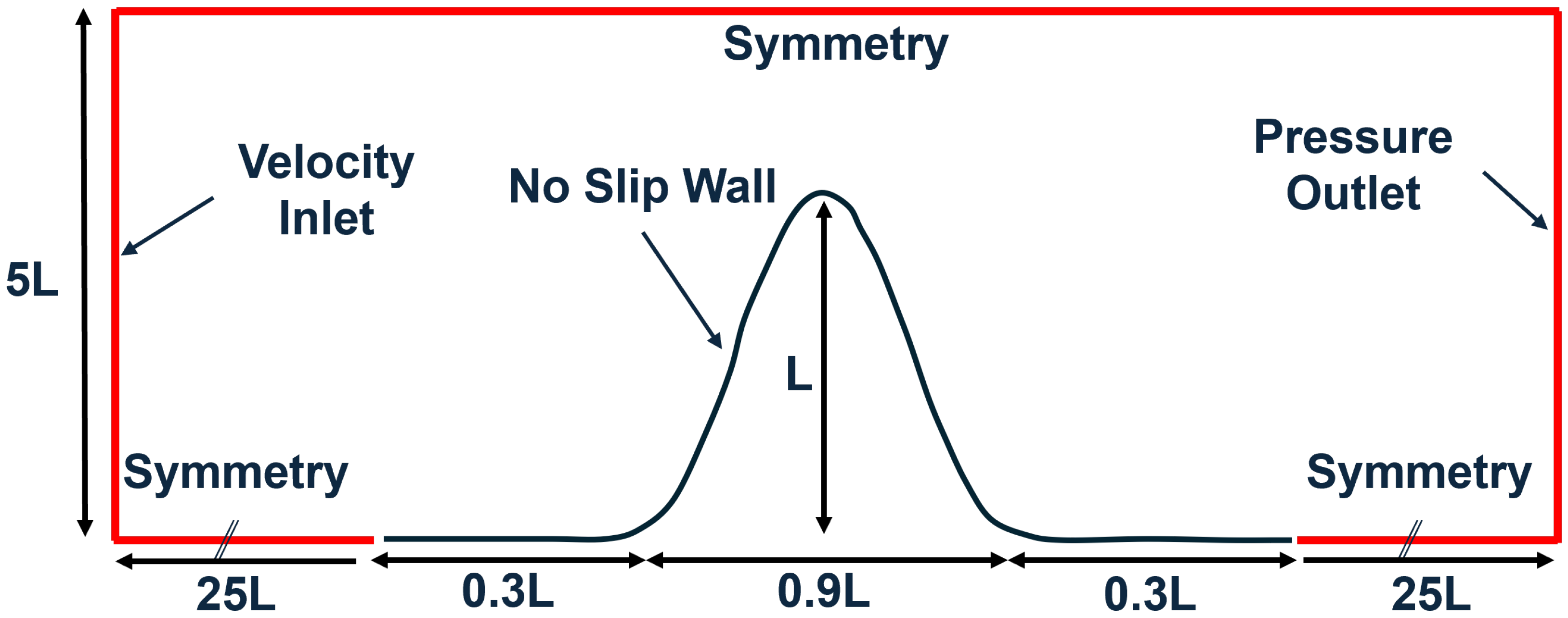
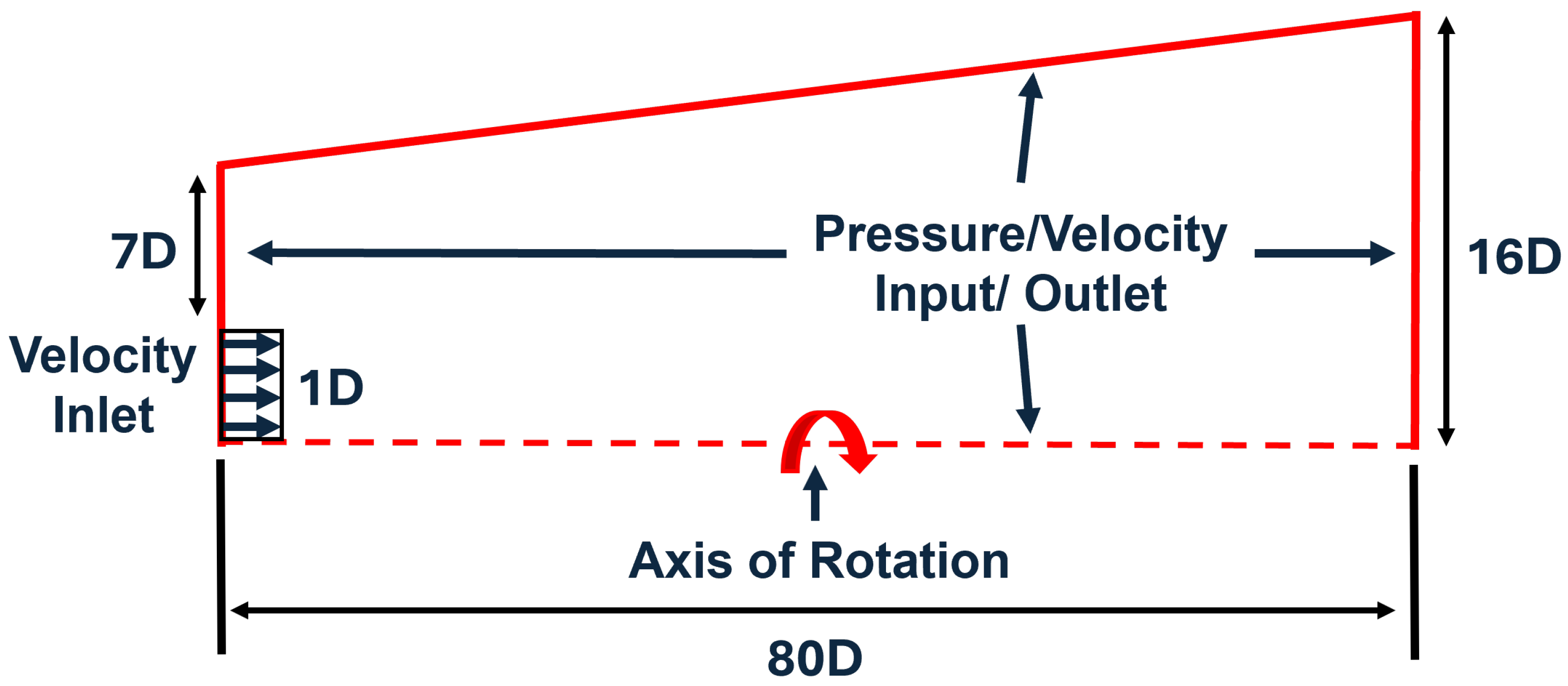
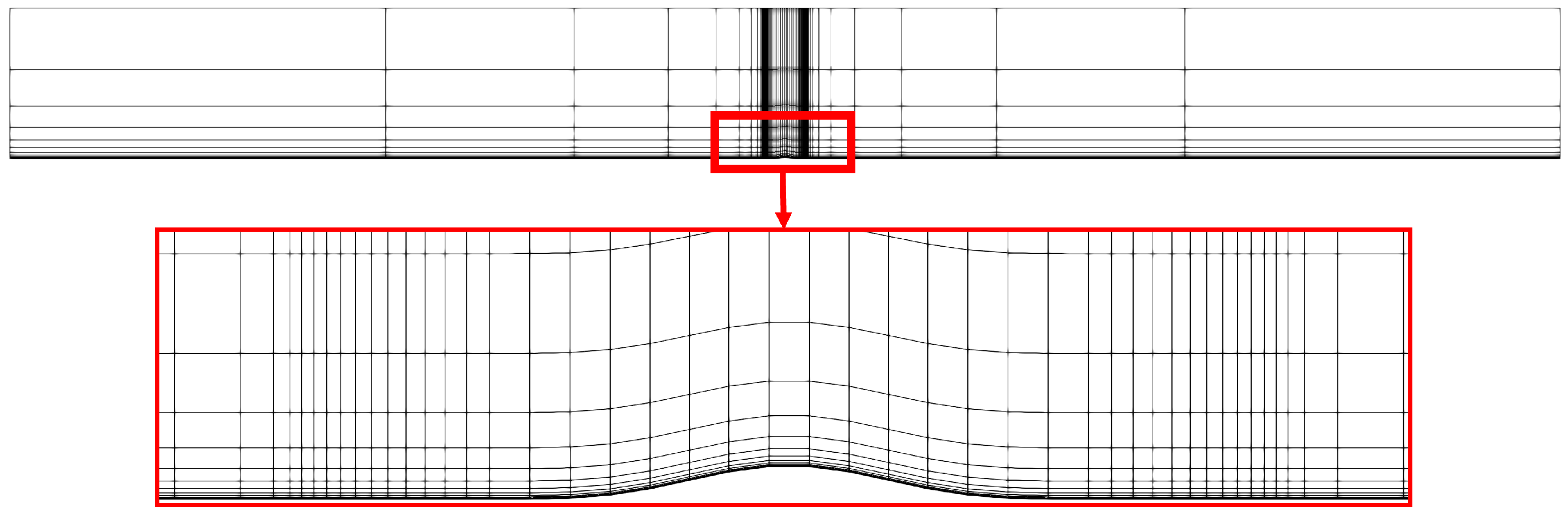
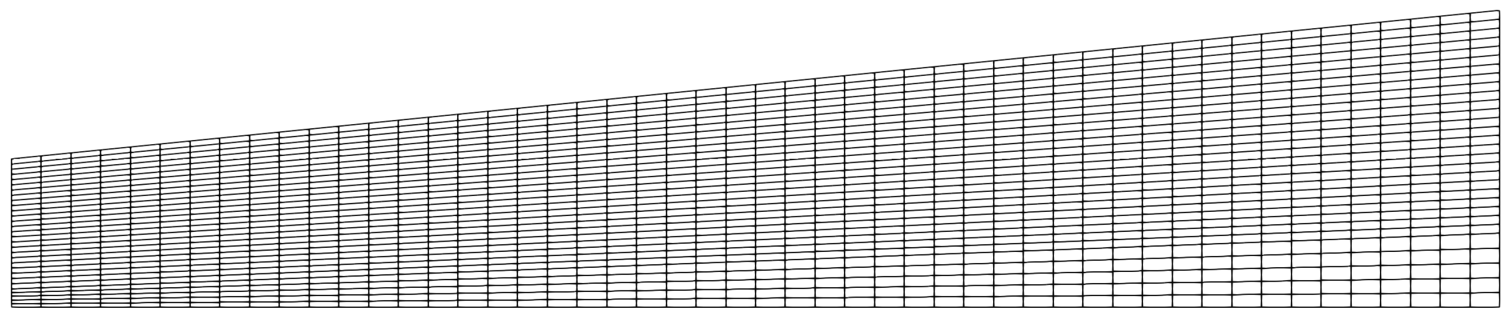
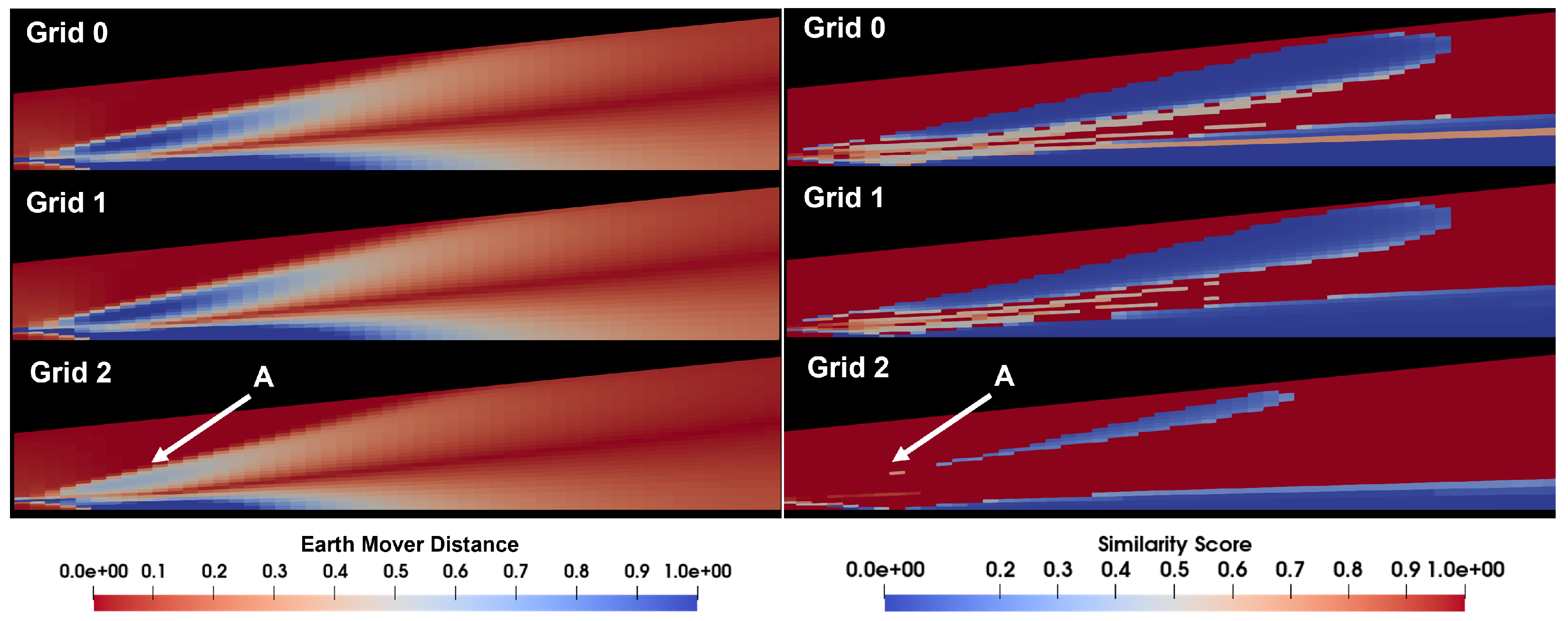
Two numerical case studies were conducted (distinct from the three flow cases discussed earlier). The first case study demonstrates the importance of specifying a convergence criterion, enabling the model to interpret the user’s definition of grid convergence. This was achieved by applying the similarity model to the geometry test cases without and with a user-defined convergence specification, and subsequently comparing the results. The second case study investigates feature selection for the model by evaluating its performance using different sets of flow features as inputs. The model was applied with various feature combinations, and its outputs were assessed against the mesh convergence results obtained earlier, as well as through visual inspection of scalar field slices.

For each case study, the model was evaluated by writing its output as an OpenFOAM scalar and displaying it along the center plane of each geometry using ParaView (v5.10.1). As mentioned previously, the similarity score ranges from 0, displayed in blue in the figures, to 1, displayed in red in the figures, where 0 is an unconverged solution while 1 is a converged solution. When analyzing the figures, the performance of the model was analyzed with two objectives in mind: intuitiveness and consistency with previous results. For the first aspect, the model was evaluated to ensure that it provides answers that are in agreement with what is known about the flow field and does not return nonsensical results. The second aspect focused on evaluating the model to ensure that its results agree with the previously performed mesh sensitivity analysis for each case and do not predict low similarity scores between two grids that have already been shown to be similar.

5.1. Similarity Score Validation

Before beginning the case studies outline above, the similarity score metric must first be checked for consistency against another statistical measure of distance to ensure its efficacy. The quantity chosen is the Earth Mover’s Distance (EM), which is a method to evaluate similarity between two distributions by calculating the amount of work required to move mass from one pile and transform it into the other pile. In this case, the piles are the probability density functions (PDF) for the selected features. To learn more about the implementation and theory, an interested reader is directed to the following works [36,37]. To compare the similarity score to the EM distance, the jet case was selected and the metrics calculated using the $U_0$ feature and the grid J3 as the focus case to compare against the other grids. The first challenge with the EM metric was that the scales between grids were seen to vary significantly. If the raw results were displayed, the EM distance appeared to show that the difference between grid J3 and J0 was the same as that between J3 and J2, which, from the mesh confirmation, has been seen to be false. To overcome this scaling, the EM score was normalized by the 95th percentile value of all of the cases calculated. This normalized score is presented alongside the similarity scores in Figure 16. Please note that for EM, a value of 0 represents perfect similarity, so the color scale on the EM scalar was flipped and clipped at a max value of 1 for display purposes. Analyzing the figure, it can be seen that the similarity score bears good resemblance to the EM distance, with both methods placing the dissimilarity regions along the jet axis and near the spread region of the jet where the flow resumes freestream behavior. The main difference between the two methods is highlighted by the annotation A of grid J2. At annotation A, it is observed that the similarity score predicts a region of almost perfect similarity while the EM distance predicts slight dissimilarity. This is believed to be due to the user feature limits that can be placed on the similarity score (to be discussed in Section 5.2 of this work). If the distance between the medians of the selected features is below a specified threshold, the similarity score will be clipped to a value of 1. In the case of the figure shown below, a limit of 0.025 was used. For other regions of the flow, the methods are seen to agree in shape with one another, but not in magnitude. From the analysis, the authors believe that the metric is grounded enough to continue for further testing.

5.2. Case Study 1: Feature Convergence Limit Specification

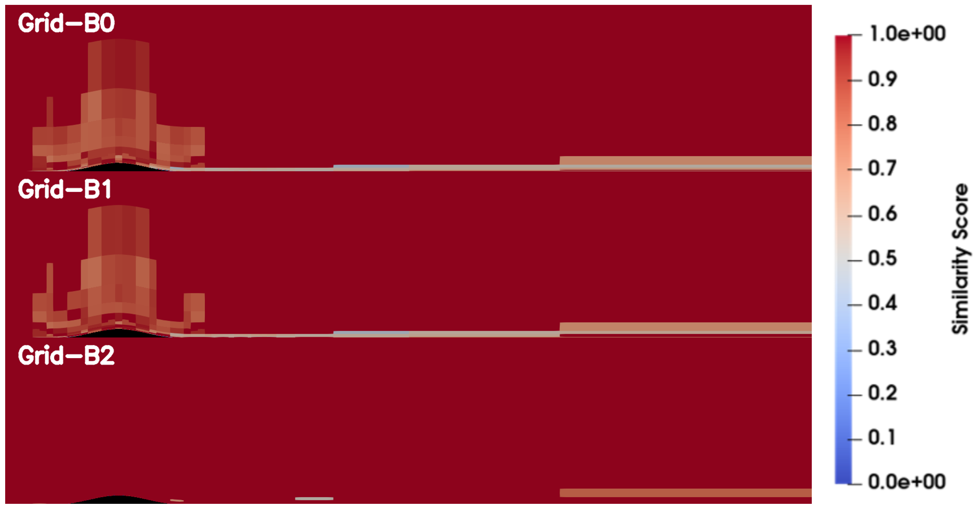
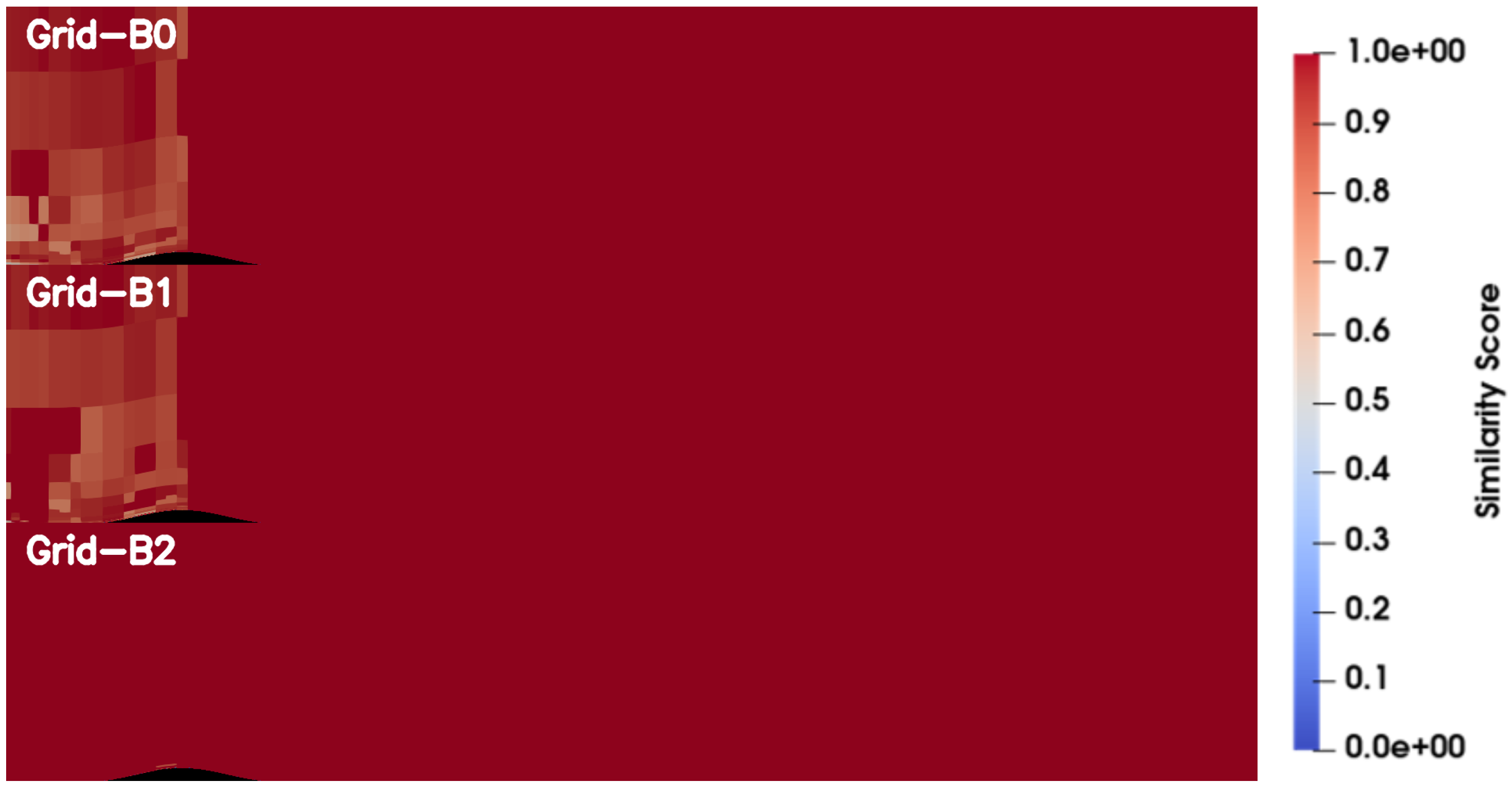
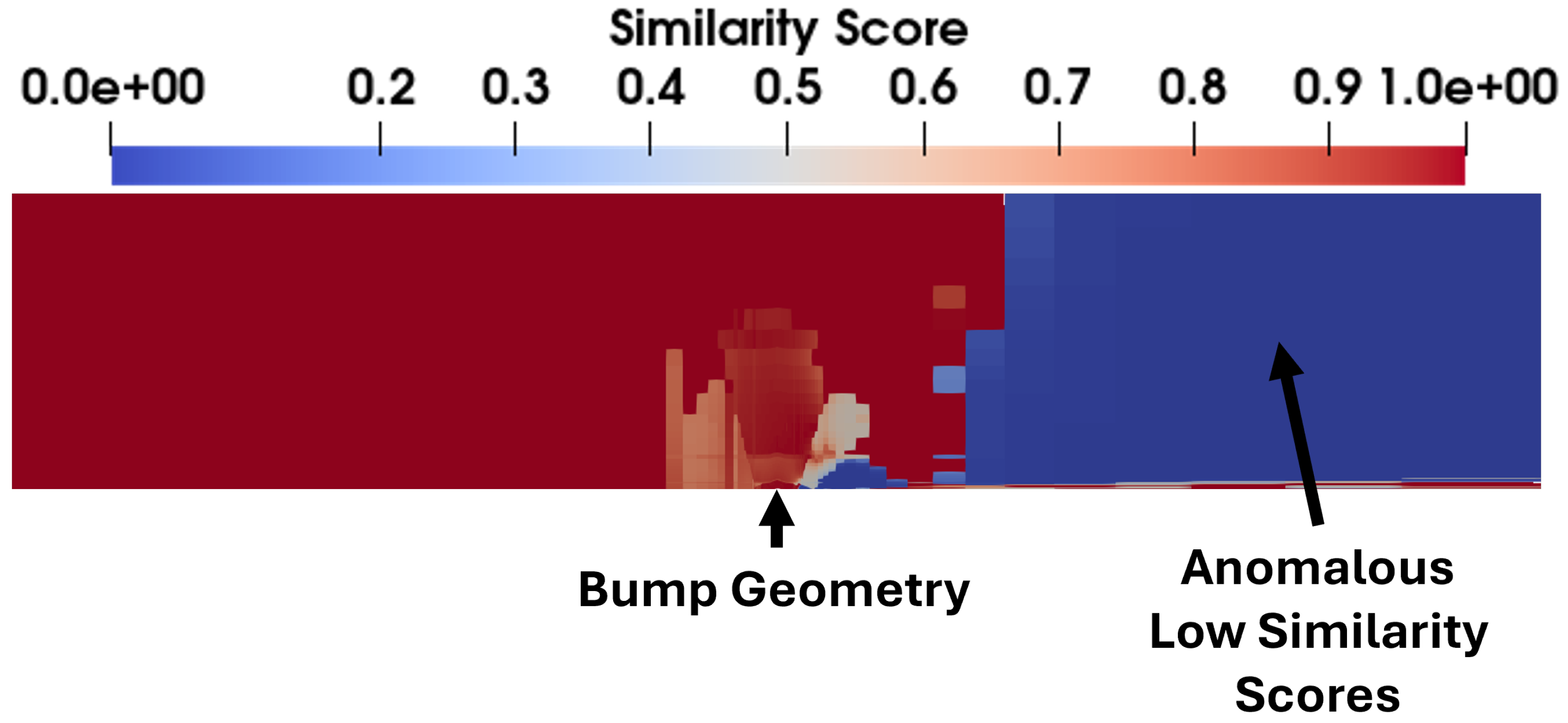
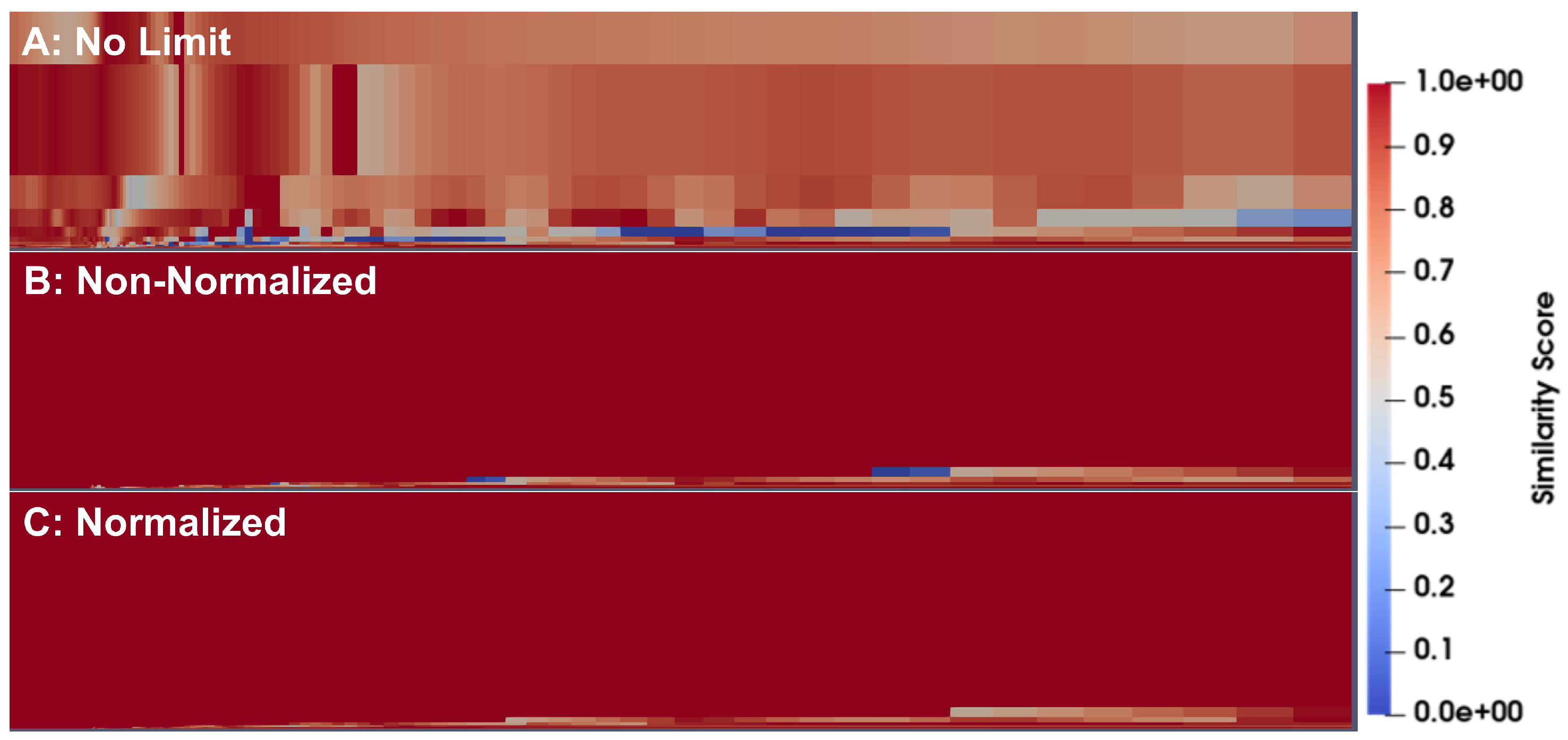
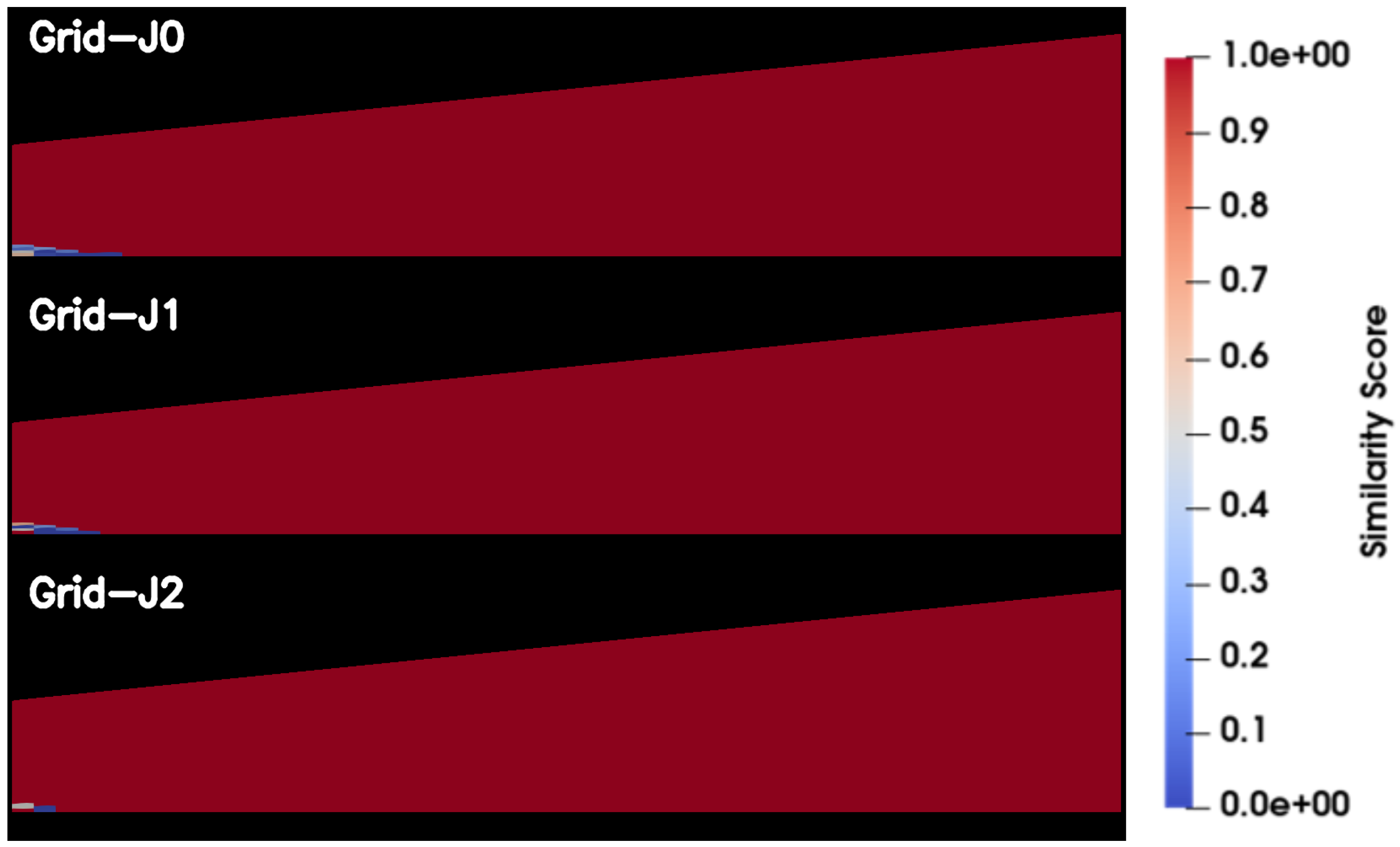
The first numerical investigation aimed to determine whether the machine-learning (ML) framework requires explicit user-defined thresholds to identify when a flow feature should be considered numerically significant. A central objective of the proposed ML methodology is to minimize user intervention. Reducing the need for expert input improves model generalizability, decreases susceptibility to user-induced bias, and allows the framework to adapt more robustly to new flow configurations. During evaluation of the model using the bump test case, however, it became evident that some degree of user-defined guidance was necessary. In particular, anomalously low similarity scores were observed in regions of the freestream that are physically unaffected by grid refinement. 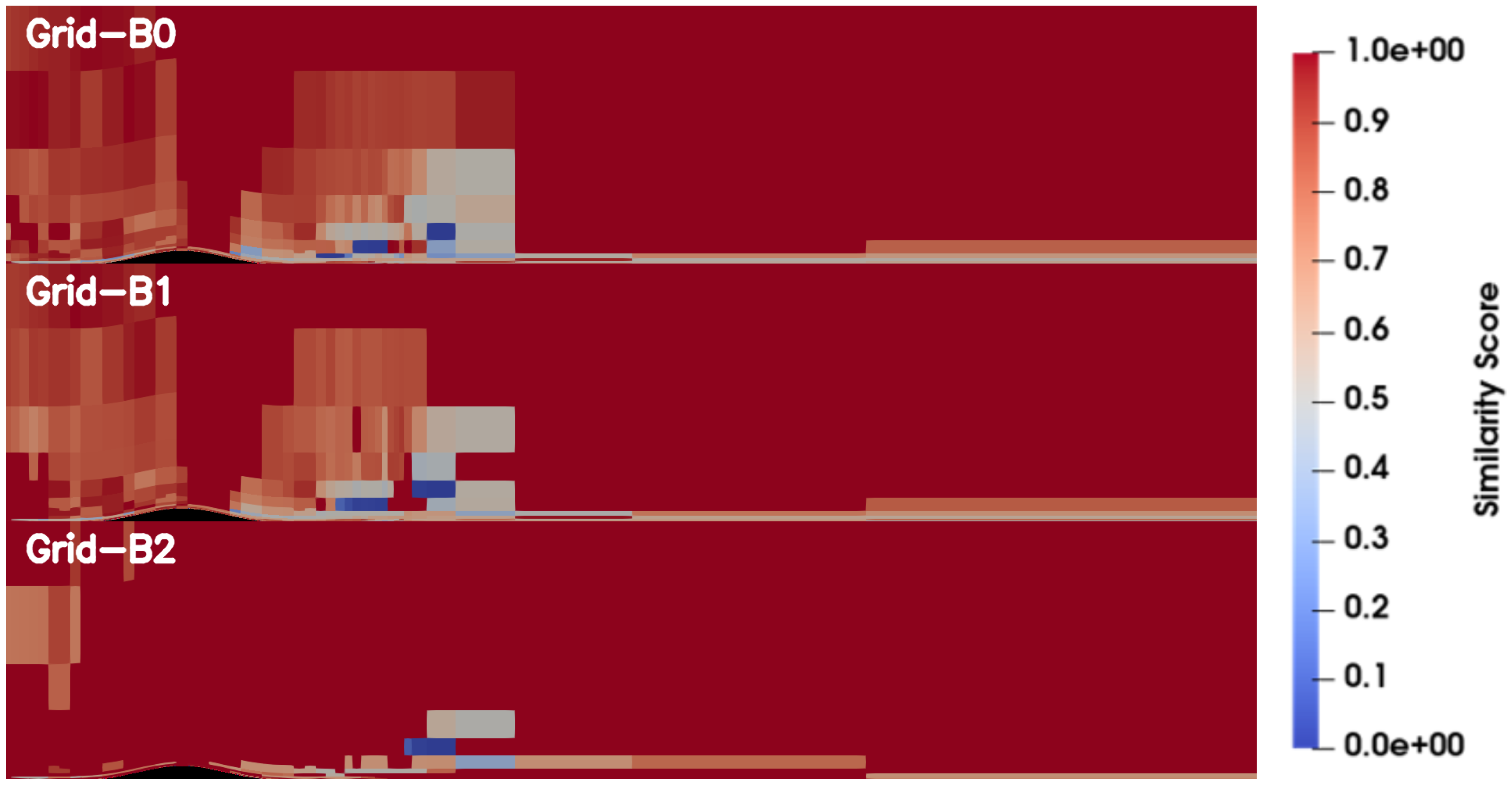As shown in Figure 17, these low-similarity zones appear far from the bump, in areas where the flow field should remain essentially invariant to mesh perturbations.Based on physical intuition and standard grid-sensitivity arguments, the solution in these regions should remain nearly unchanged with grid refinement. Since there are no strong gradients or localized features, the similarity scores should be close to one. Further examination revealed that the ML model exhibited excessive sensitivity to small-magnitude variations in the feature fields. This scale sensitivity led the model to assign disproportionate importance to numerically insignificant fluctuations, thereby producing artificially low similarity values in otherwise uniform regions. These findings indicate that, without appropriate magnitude-based normalization or user-defined tolerances, the model may misinterpret benign numerical noise as physically meaningful deviations.

In the anomalous regions shown in Figure 17, the model detected differences between the two grids, but the changes in feature magnitude were extremely small. In this example, the feature under consideration was the $U_0$ velocity component, and the average difference between the grids in these regions was approximately 0.01%. Despite the small magnitude, the model identified this variation and separated the grids into distinct clusters, resulting in a low similarity score. However, the model did not recognize that, although the distributions differed slightly, the magnitude of the change was so small that it would be considered insignificant by a human observer. This limitation is not a failure of the model itself, since it was never provided with information about which differences should be treated as meaningful. To address this issue in the baseline model, a mechanism was introduced to allow the user to define a feature validity limit. This limit is applied by evaluating each feature using Equation (24), where ${\beta }^i$ is the validity threshold for the i-th feature, $X_{j/k}^i$ is the corresponding feature set, Med is the median, and j/k represent the two grids being used in the calculation.

$$Med\left(X_j^i\right)-Med\left(X_k^i\right)\ge {\beta }^i$$

(24)

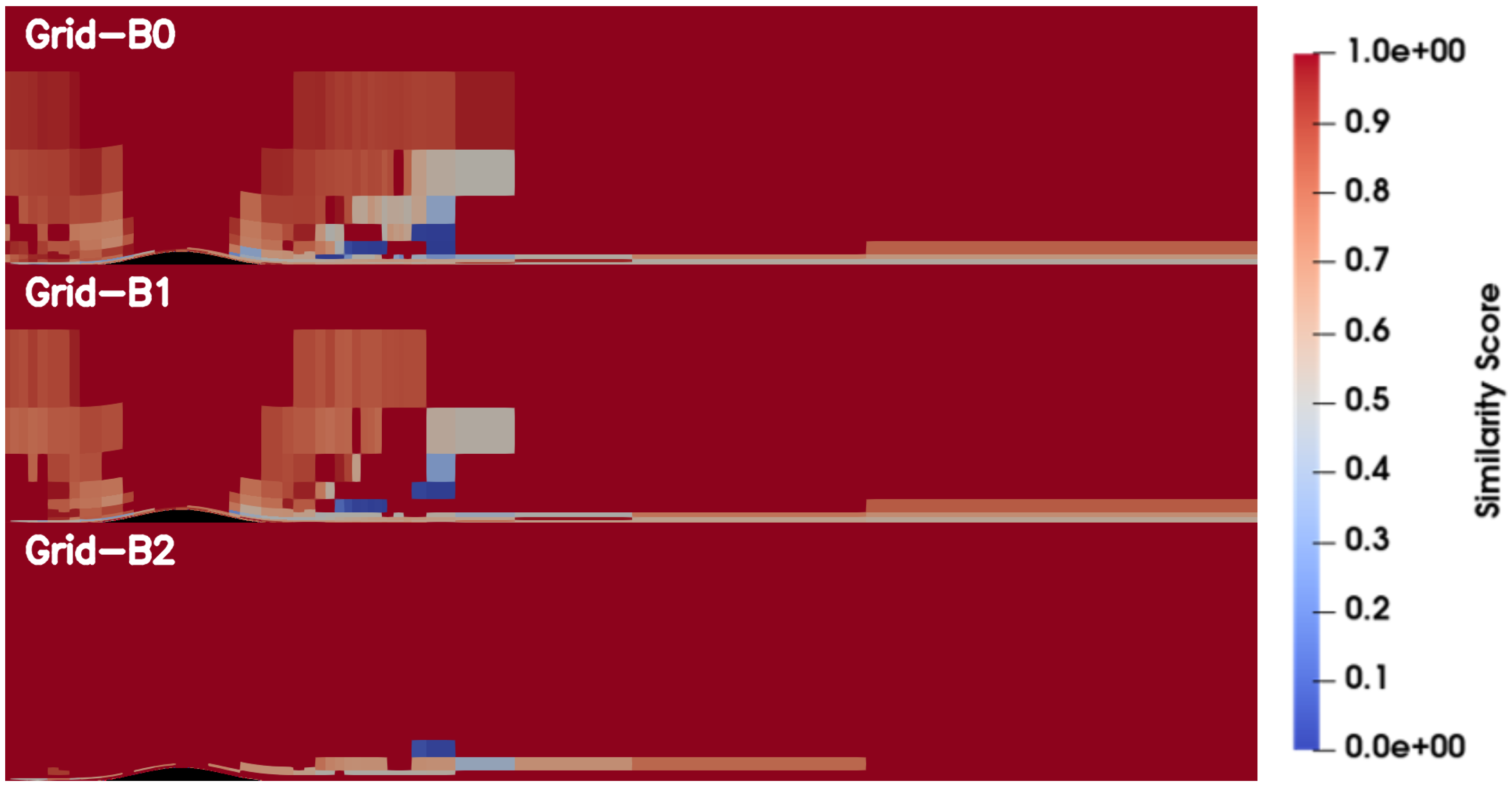
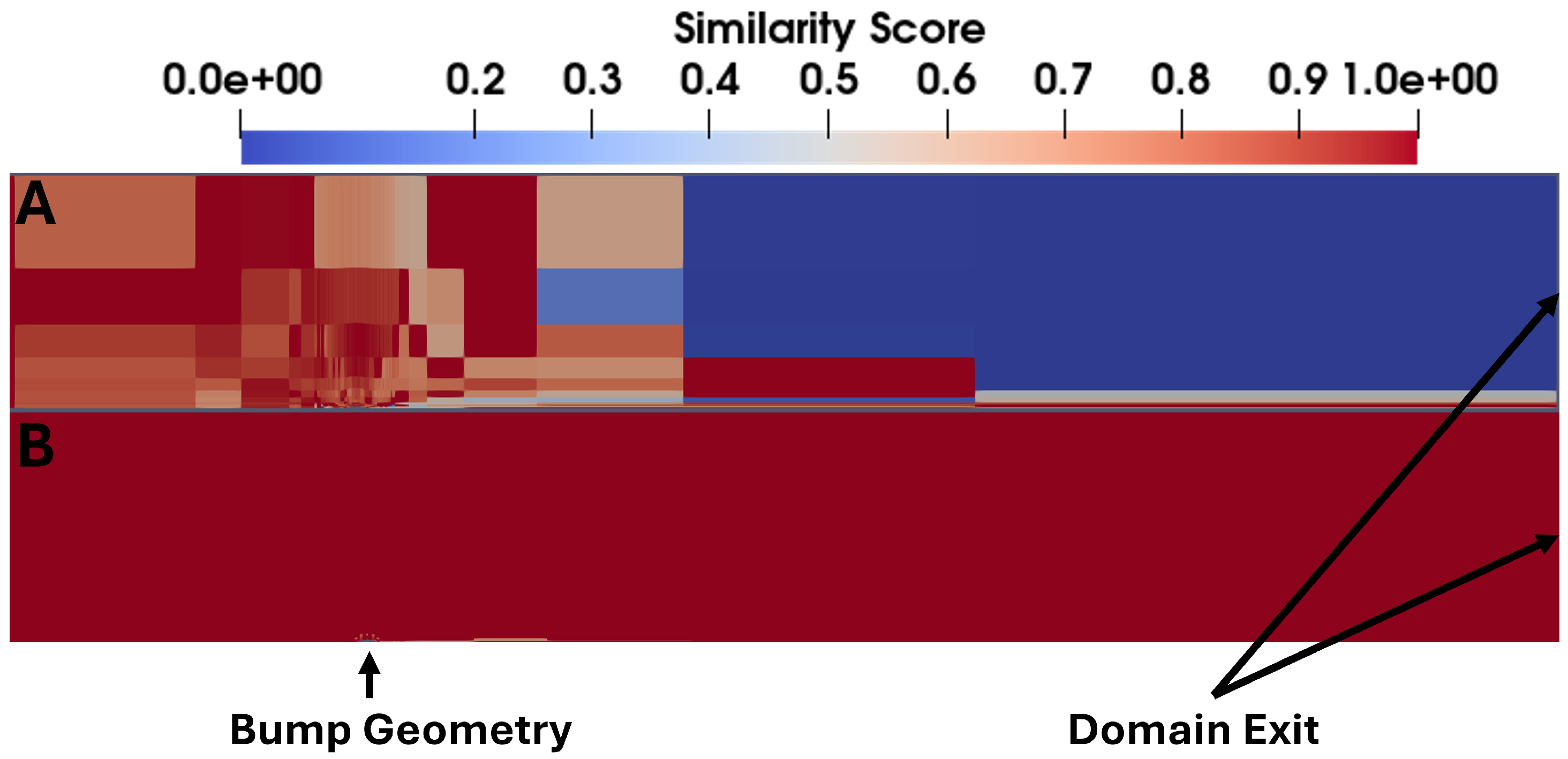
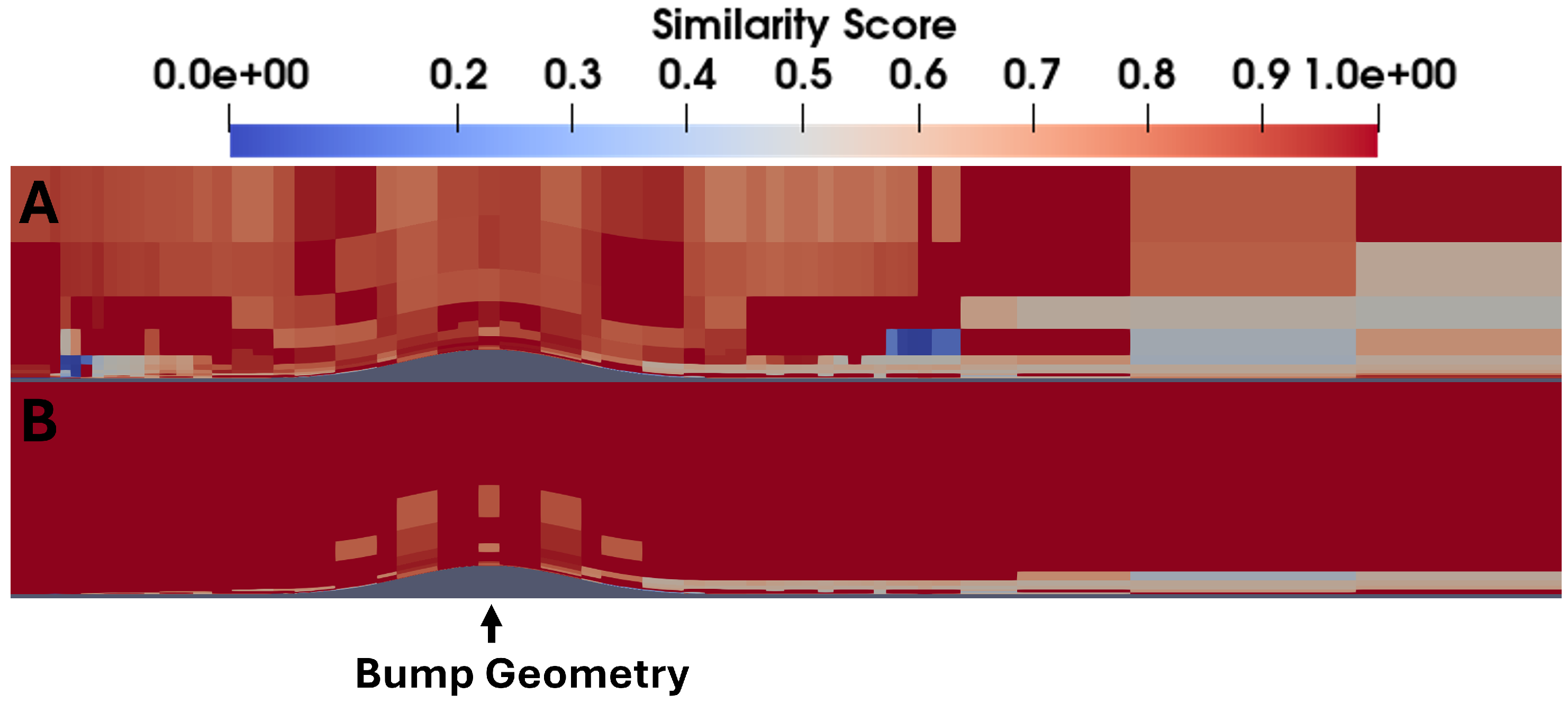
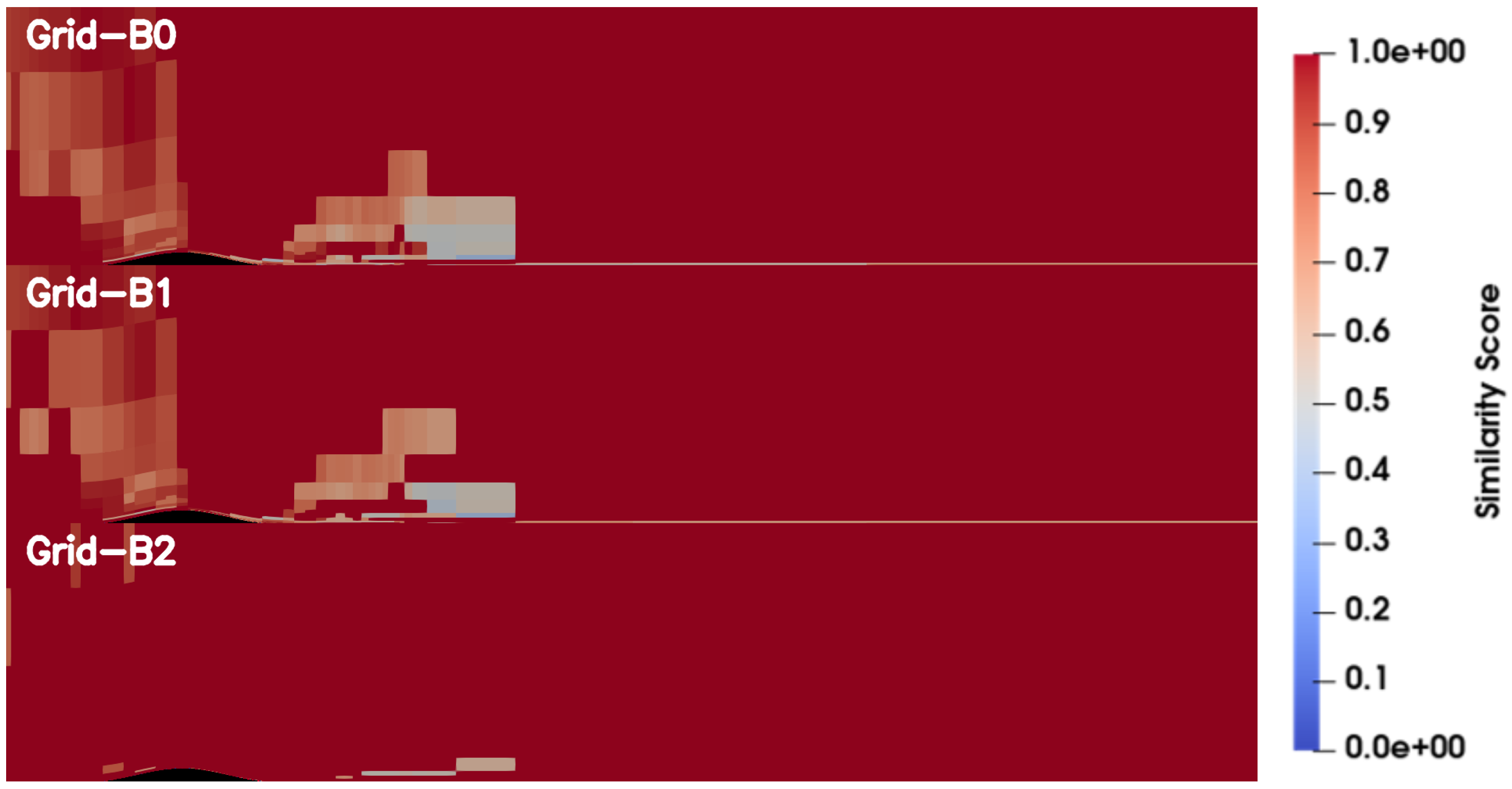
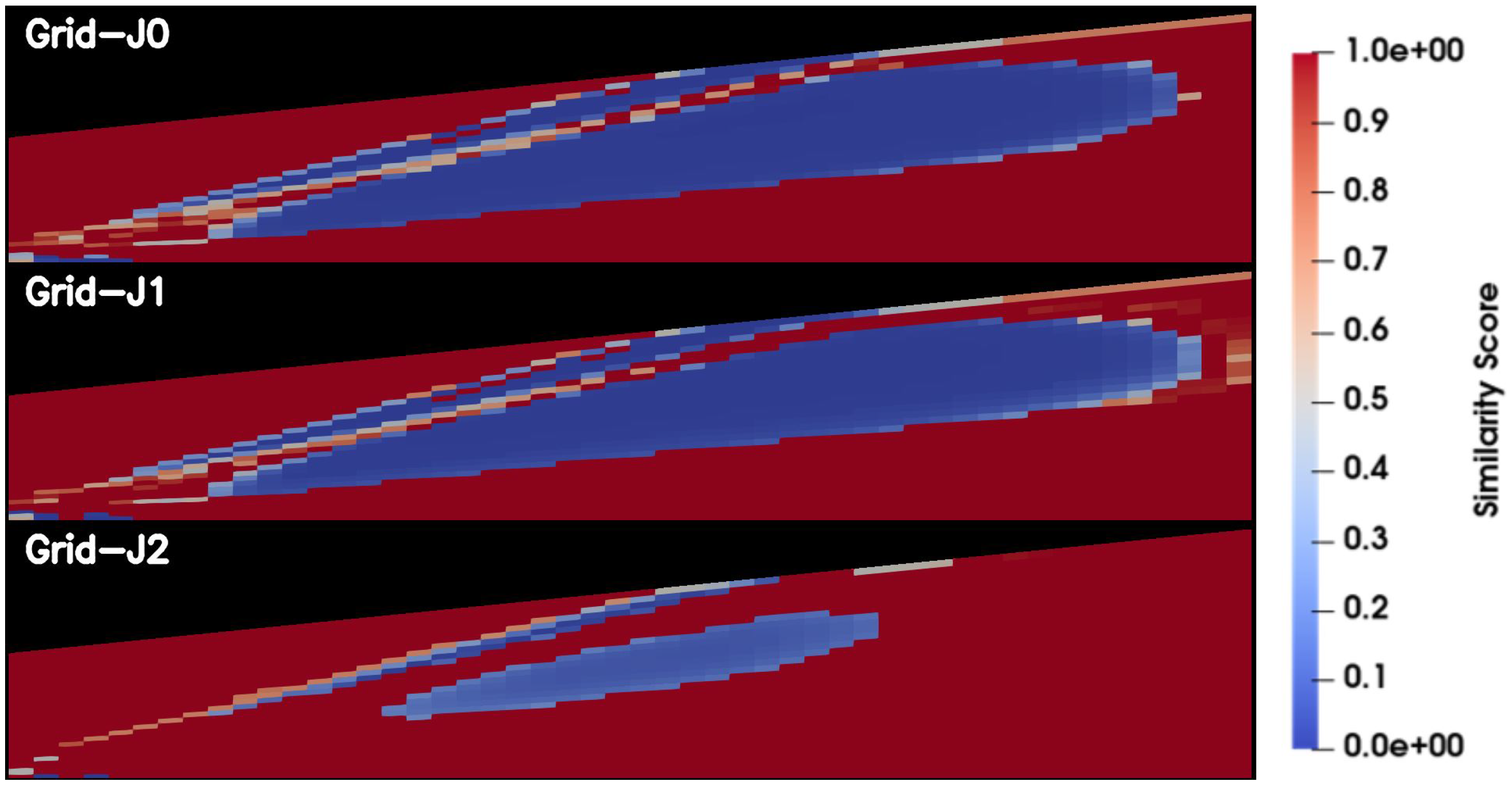
If a feature fails to satisfy the validity criterion in Equation (24), it is considered converged by user definition and is removed from the feature set provided to the ML model. If none of the features pass the validity test, the model is left with an empty feature set, and the similarity score is manually assigned a value of 1, since all features are deemed to have converged. Figure 18 and Figure 19 illustrate the implementation of this feature-validity check using the streamwise velocity for the 2D bump-in-channel case. Pane A in both figures shows the similarity score computed without a feature-validity check, whereas Pane B shows the score after applying the validity criterion. In Figure 18, the validity check clearly eliminates the spurious low-similarity regions in the far field. When zooming into the bump region in Figure 19, it becomes evident that the validity check isolates the only physically significant differences between the grids to the vicinity of the bump, which is the expected behavior.

Absolute limits also allow users to introduce custom normalizations that may be better suited to a specific problem. For example, one may normalize the velocity-gradient feature by the local velocity, $(\partial U_0/\partial x_0)/U_0$ (Here, $x_0$ and $x_1$ denote the streamwise and normal directions, respectively.). This type of normalization enables the user to define an absolute limit in terms of a physically intuitive quantity—namely, “the fractional change in velocity per unit distance”. Such an interpretation is straightforward to understand and directly relevant to many flow problems. Figure 20 compares two approaches applied to the $\partial U_0/\partial x_1$ feature: no limit implementation and an absolute limit implementation using the normalized gradient $\left(\partial U_0/\partial x_1\right)/U_0$. The results show that both approaches perform effectively when the absolute limit is paired with a feature that is properly scaled across the domain.

This case study highlights the importance of having users define for the model what they consider a “converged” feature. If users do not specify the level of change they regard as converged, the model tends to be overly sensitive to minor variations in the flow field. These minor changes can significantly affect the similarity scores, leading to artificially low scores in areas that are mostly unaffected by grid refinement. To address this issue, the introduction of feature checks using the $\beta$ parameter has proven to be an effective solution for eliminating non-physical similarity scores. The use of a feature limit was found to be problematic for features that do not scale throughout the domain and can result in excessively high similarity scores. In these cases, the user must provide an intuitive scaling for the feature throughout the domain.

From case study one, it was observed that the choice of $\beta$ plays a role in the final similarity score. While the model is sensitive to the value of $\beta$, the choice of $\beta$ is intuitive since it is based purely on what the user would deem to be a significant value. When setting a value for $\beta$, the user needs only to answer the following question, “If the difference in median values between the two cases was below $\beta$, would I consider them significantly different?” By answering this question, the user conveys to the model what a human would consider a convergence value, meaning that while the model is influenced by the value of the parameter, it is not a value that must be tuned through complex search methods. 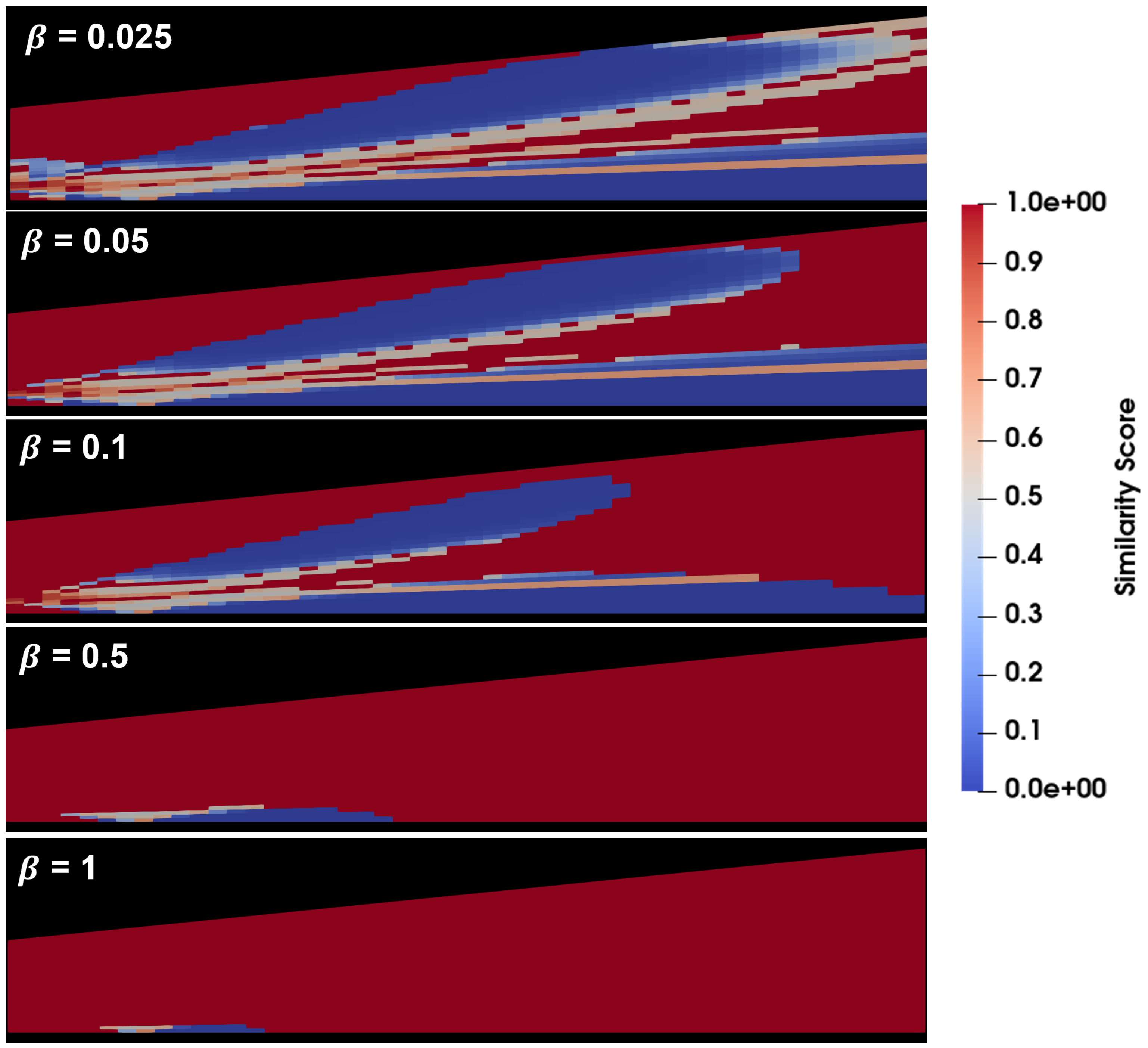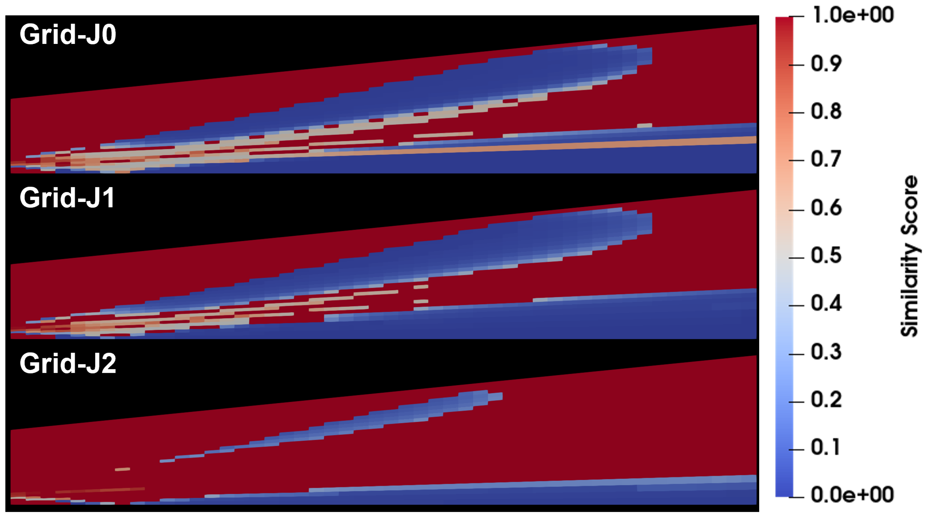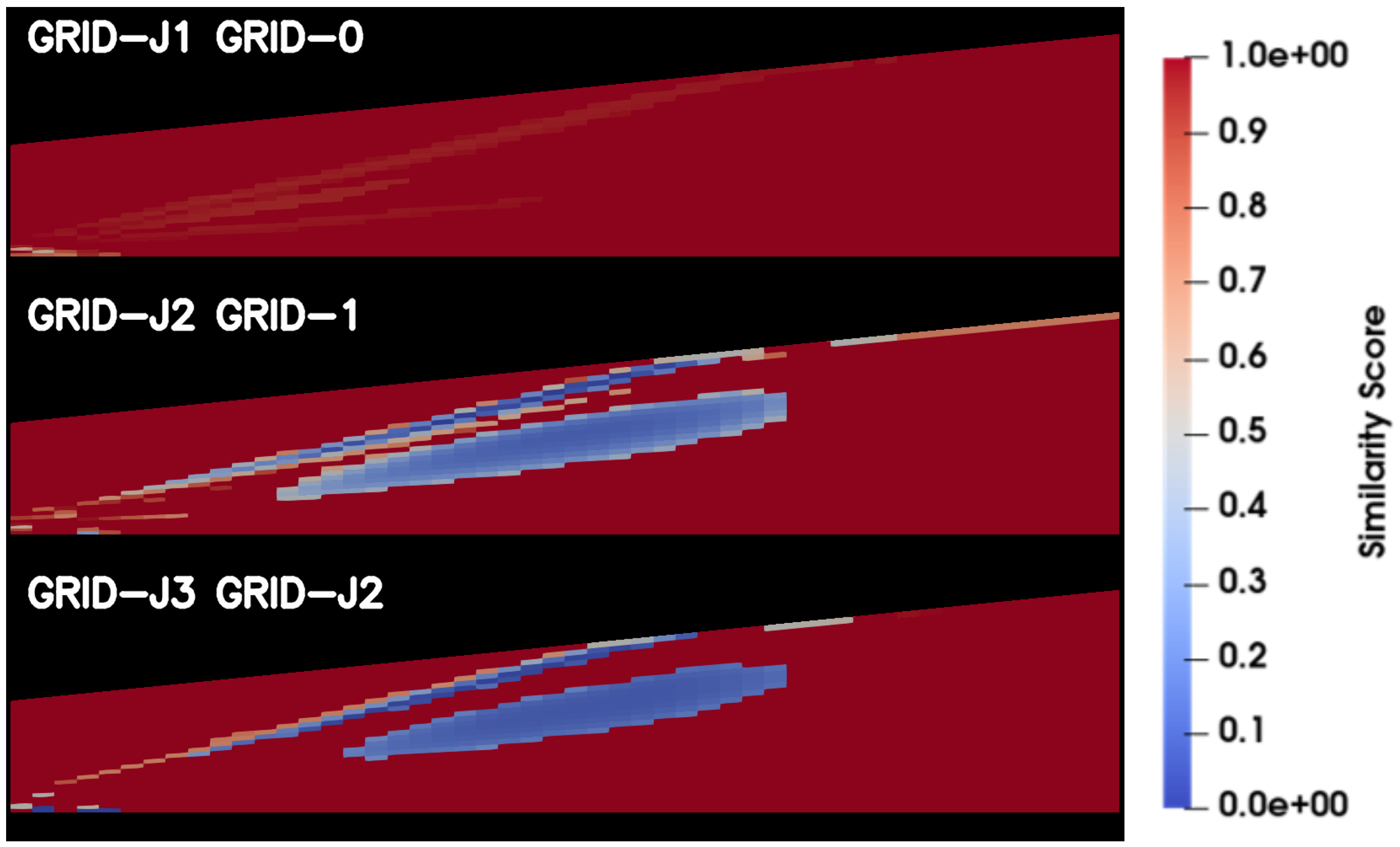To help the reader better understand the influence of the $\beta$ parameter on the solution, Figure 21 shows a sweep of the $\beta$ parameter. The jet grids J3 and J0 were used to calculate the similarity score for the feature $U_0$ while sweeping the $\beta$ from 0.025 to 1. The figure demonstrates that as the parameter is increased, the regions of dissimilarity are reduced with only the strongest regions, those along the jet axis, remaining at $\beta =0.5$ and $\beta =1$.

5.3. Case Study 2: Feature Selection

The second numerical experiment focused on examining feature selection within the model. Since the framework is designed to accept any flow variable as input for computing similarity, an important question arises: which features provide the most meaningful and physically consistent results? In this context, a “better” feature is defined as one whose similarity trends align closely with the convergence behavior observed in standard mesh-confirmation analyses and whose response clearly and intuitively differentiates between grid levels. To investigate this, the axisymmetric jet and bump geometries were used as test cases. Five different feature sets were evaluated using the similarity model with the feature-validity criterion applied. The selected features were the streamwise velocity $U_0$, the transverse velocity $U_1$, the velocity gradients $\partial U_0/\partial x_0$ and $\partial U_0/\partial x_1$, and the combined gradient set $\{\partial U_0/\partial x_0,\partial U_0/\partial x_1\}$.

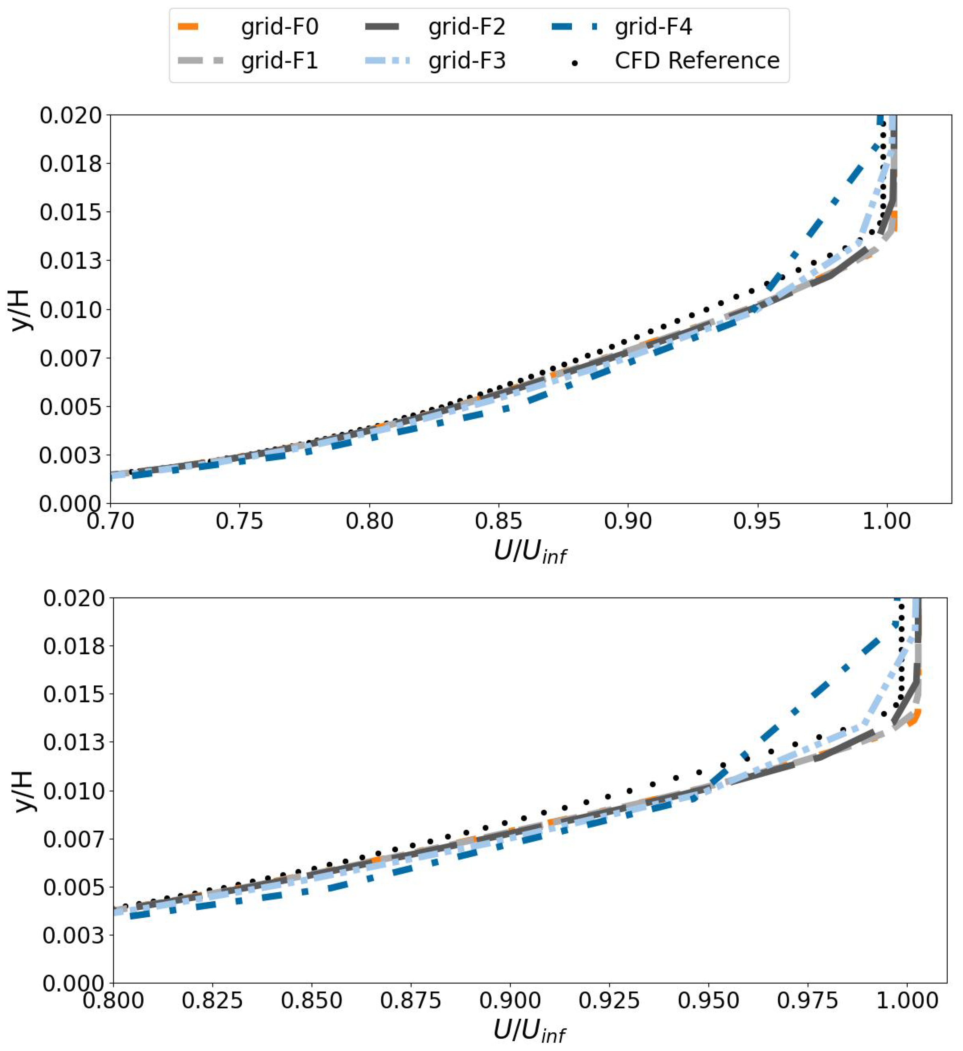
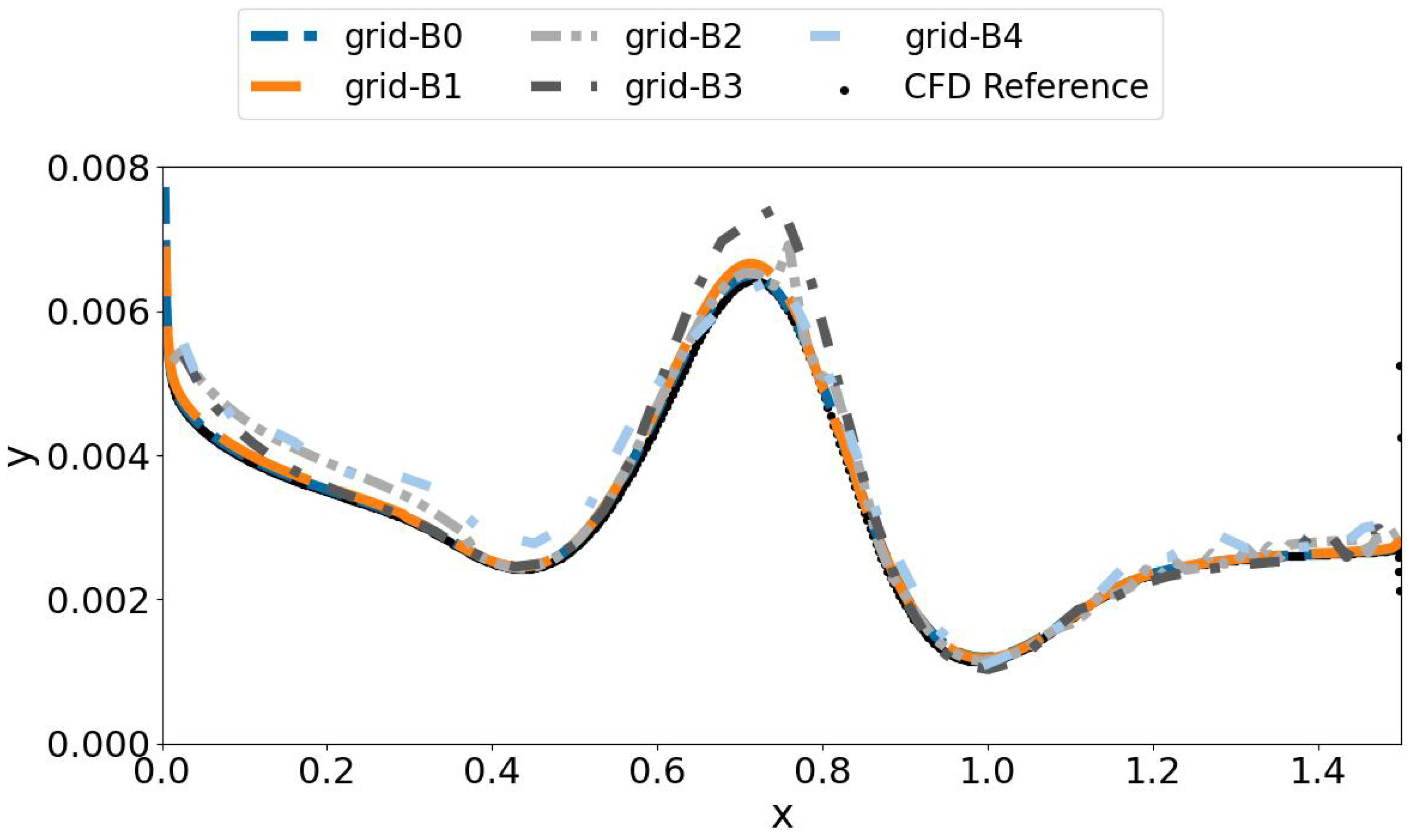
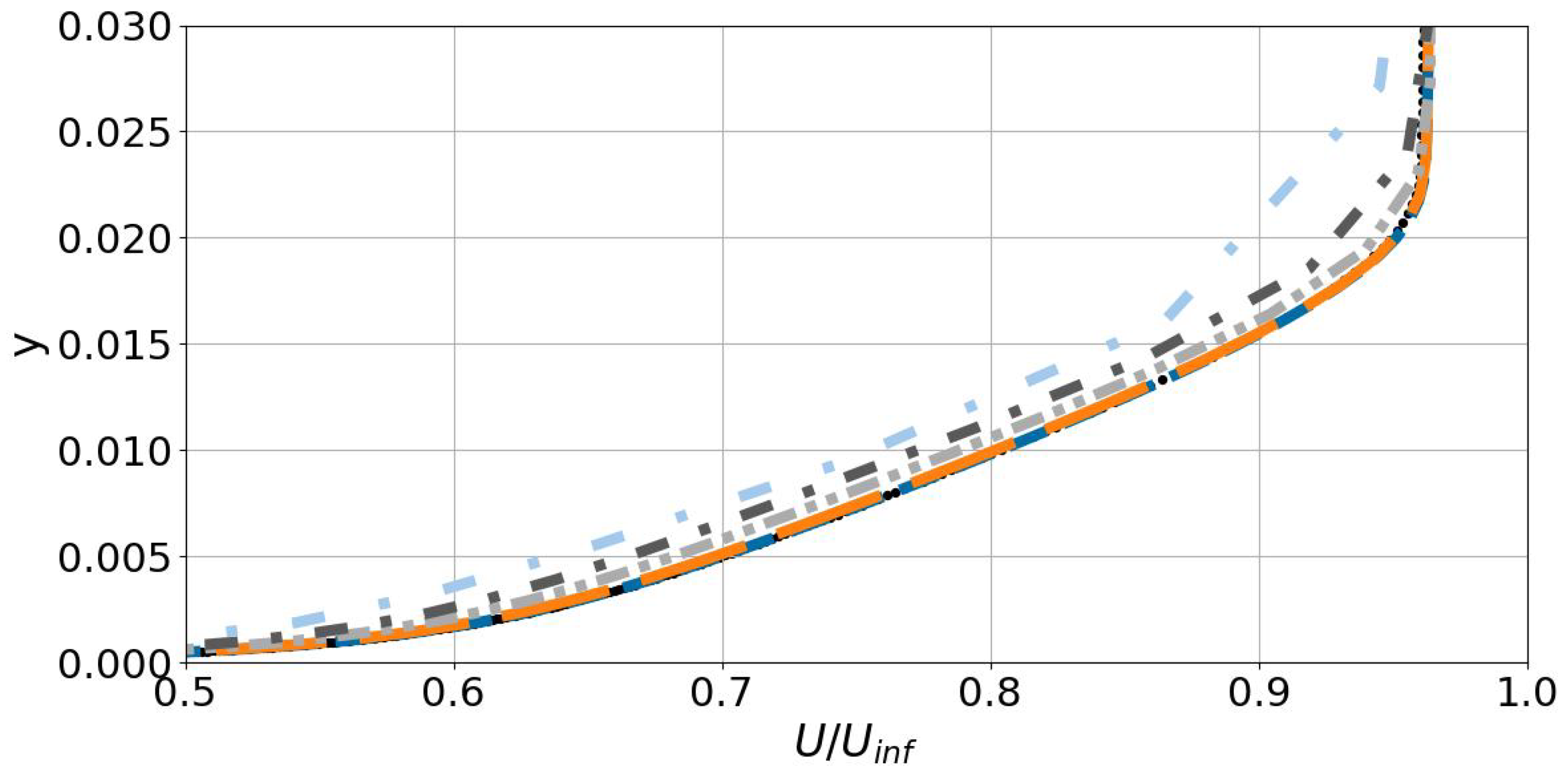
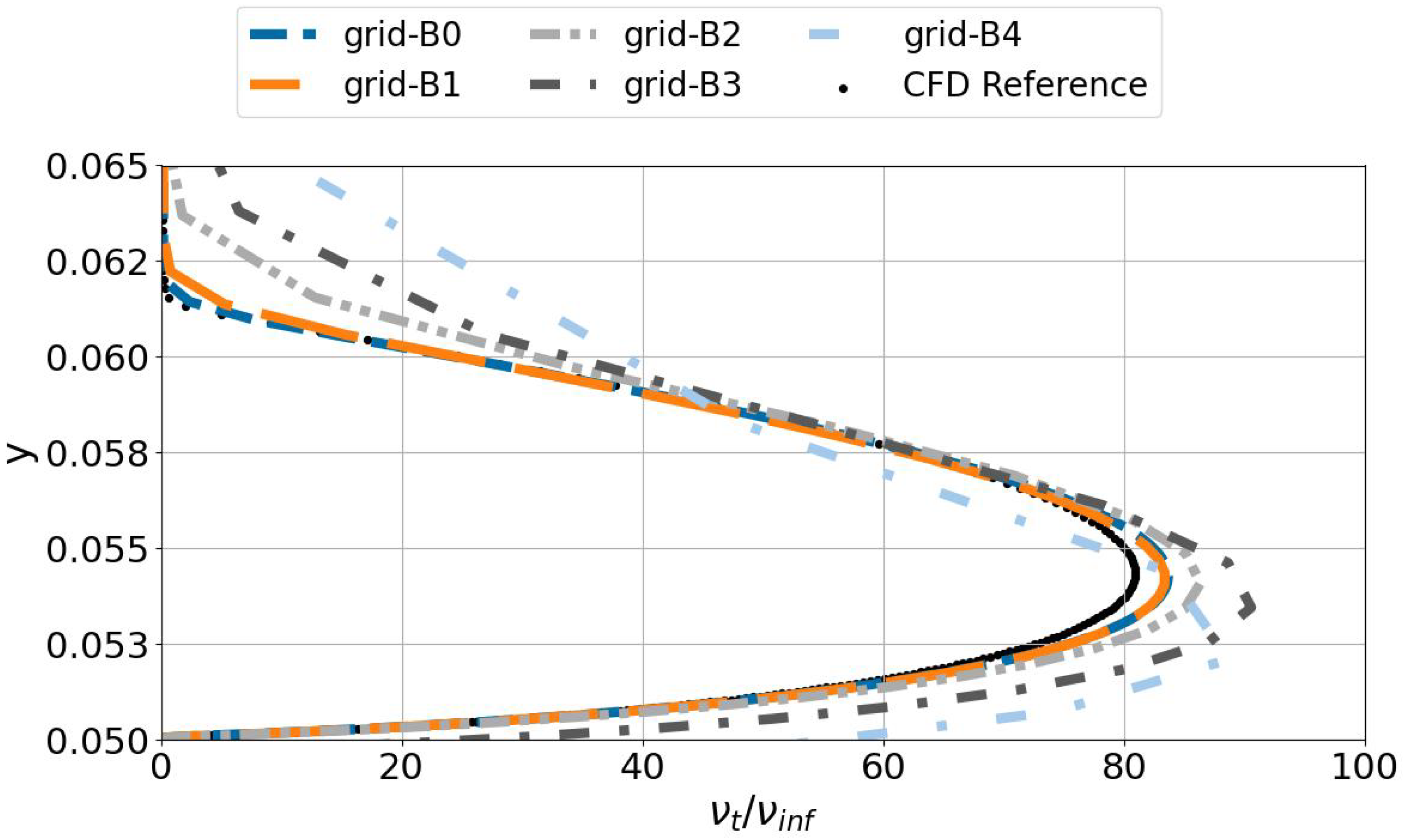
We begin the feature-selection analysis with the bump cases. Before examining the similarity results, a brief summary of the mesh-confirmation study is helpful. Analysis of the skin-friction, velocity, and eddy-viscosity profiles in the bump wake showed substantial differences between grids B3 and B2, smaller differences between B2 and B1, and virtually no change between B1 and B0. Based on these findings, comparisons involving grid B3 should yield the highest similarity with B2, with progressively lower and nearly indistinguishable similarity scores when compared with B1 and B0.

Figure 22 and Figure 23 present the similarity fields for the bump case using the $U_0$ and $U_1$ velocity components, respectively. In both cases, the expected trends from the mesh-confirmation study are reproduced, with B3 and B2 showing nearly identical similarity levels. However, using velocity alone as the feature does not highlight the differences between B3 and B2 as strongly as one might anticipate. This behavior can be understood by examining the velocity profiles in Figure 12, where $U_0$ reaches its freestream value by $x_1=0.025$. Consequently, most of the mesh-dependent variation occurs close to the wall, which is not fully captured in the plotted slices. The $U_0$ feature set identifies differences between B3 and the finer grids primarily around the bump and in the near-wall region of the far wake. In contrast, the $U_1$ velocity component detects differences mainly from the leading edge of the bump up to its apex, reflecting the physical structure of the flow in that region.

Extending the feature analysis to the gradients, Figure 24, Figure 25, Figure 26 and Figure 27 show the ML results for the individual velocity gradients $\partial U_0/\partial x_0$ and $\partial U_0/\partial x_1$, and the combined gradient set $\{\partial U_0/\partial x_0,\partial U_0/\partial x_1\}$. Starting with the $\partial U_0/\partial x_0$ feature, it can be seen that once again the model does a good job at providing almost identical predictions for grids B1 and B0. The $\partial U_0/\partial x_0$ feature agrees with the velocity features in the respect that it shows very little difference between grids B3 and B2. The $\partial U_0/\partial x_0$ does show some difference between the B3 grid and the B1 and B0 grids in the near wake, but not in the far wake, like the velocity features.

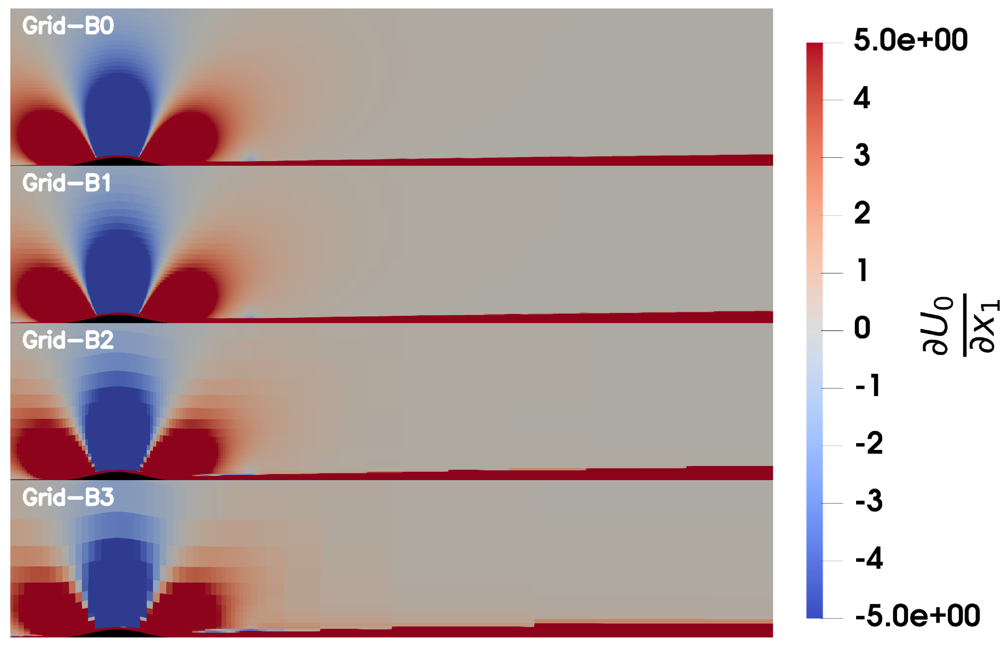
The $\partial U_0/\partial x_1$ feature set, shown in Figure 25, is the first to reveal a clear distinction between grids B3 and B2. The transverse velocity gradient in the $x_1$ direction highlights more pronounced differences between B3 and the finer B1 and B0 grids than any of the previously examined features. This behavior is further illustrated in Figure 26, which displays the $\partial U_0/\partial x_1$ field at the same locations used for the similarity slices. In this figure, one can see that grids B3 and B2 smear the gradients directly over the bump, producing a noticeably different distribution from that of the finer meshes. The coarse grids also generate a small pocket of negative $\partial U_0/\partial x_1$ immediately downstream of the bump, while this feature is absent in the B1 and B0 solutions. In the far wake, B3 and B2 exhibit near-wall gradient structures that differ substantially from those in B1 and B0. Both of these mesh-dependent discrepancies, near the bump and in the downstream region, are well captured by the model’s similarity predictions, demonstrating the sensitivity of the gradient-based feature to physically meaningful changes in the flow.

Finally, the $\partial U_0/\partial x_0$ and $\partial U_0/\partial x_1$ fields were combined into a single feature set and input to the model. The resulting similarity predictions are shown in Figure 27. This combined-gradient feature set produces the widest range of similarity scores among all the cases examined. It is important to note that the resulting field is not simply a linear superposition of the outputs obtained from the individual $\partial U_0/\partial x_0$ and $\partial U_0/\partial x_1$ features. Instead, the combined input retains the dominant trends seen in both individual feature sets while amplifying regions of dissimilarity, particularly in the B3 to B2 comparison. This suggests that combining complementary gradient information provides a more sensitive indicator of mesh-dependent flow variations.

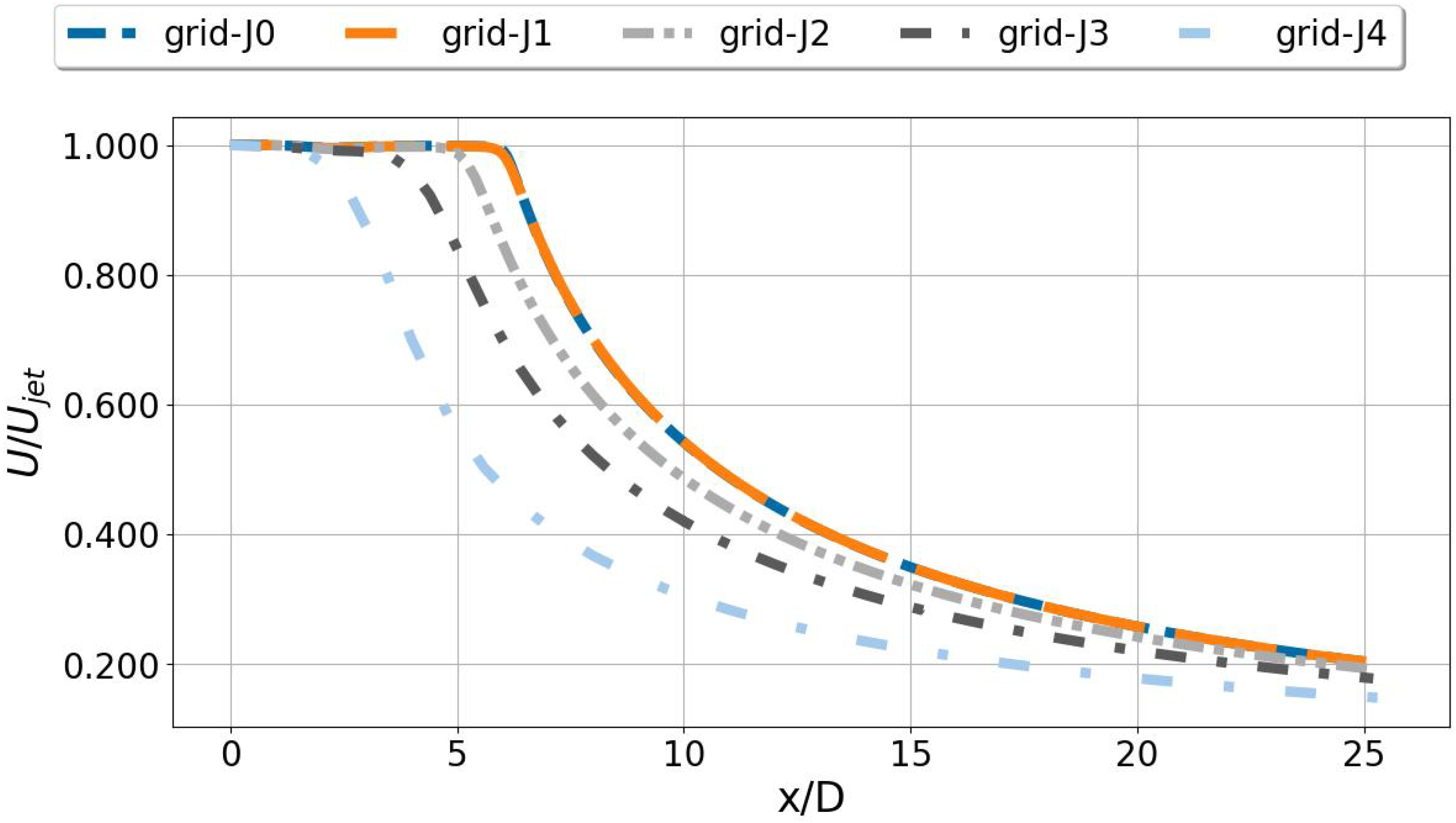
To continue the feature-selection analysis, the following figures compare grid J3 of the jet case with grids J2, J1, and J0 using each of the feature sets. Before examining these results, it is helpful to summarize the expectations based on the mesh-confirmation study presented earlier. The analysis showed substantial differences in both the centerline and radial velocity profiles between successive grids until J1 and J0, whose profiles nearly overlapped. Accordingly, when evaluating the similarity predictions, we expect grid J2 to appear most similar to J3, while grids J1 and J0 should yield nearly identical similarity fields. The mesh-confirmation study also revealed that differences in the radial streamwise velocity profiles became more pronounced farther downstream from the jet inlet, a trend that should be reflected in the similarity distributions.

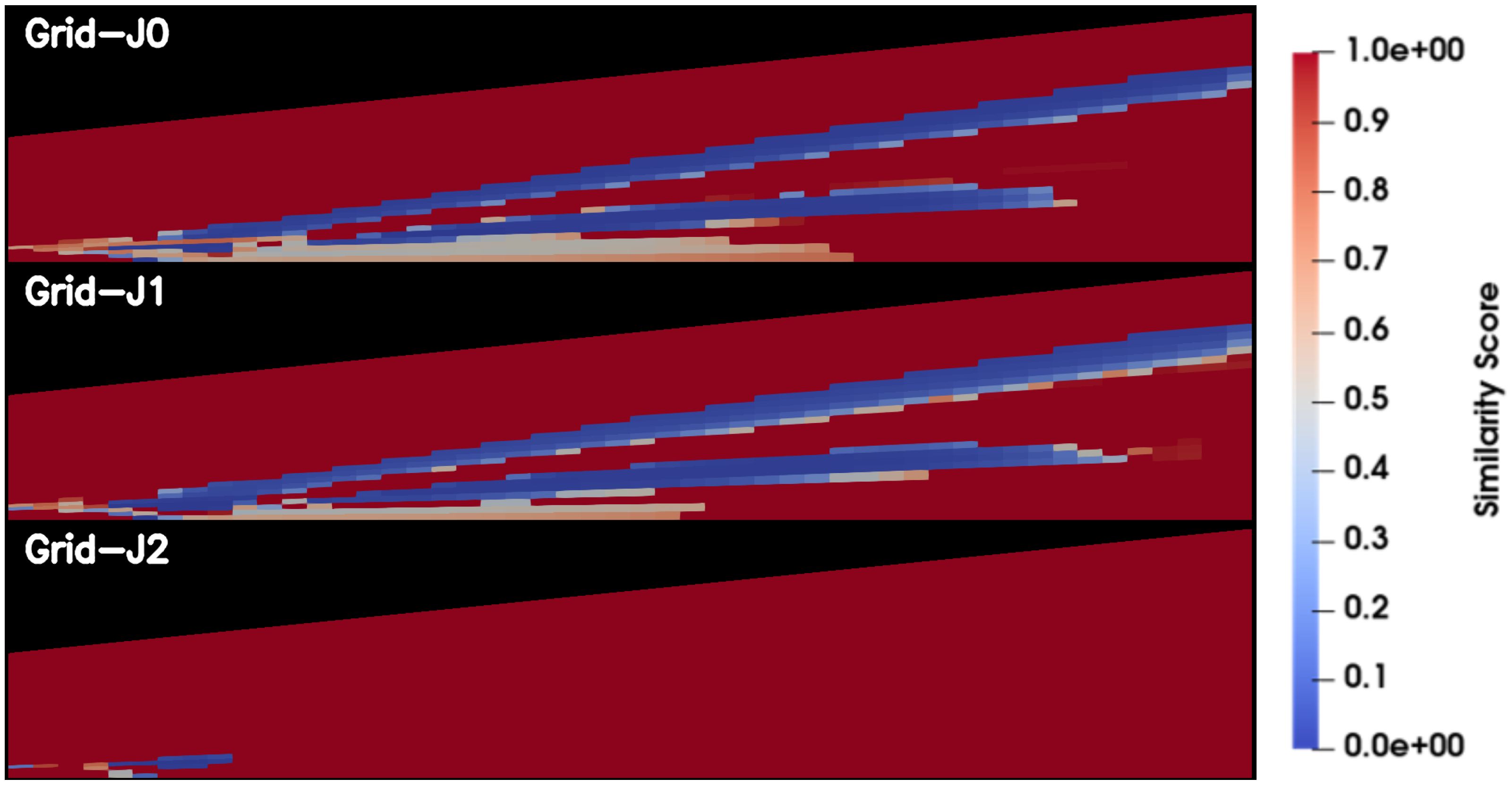
Figure 28 and Figure 29 present slices of the jet domain with similarity scores computed using the $U_0$ and $U_1$ velocity components as features, respectively. The most prominent difference between the two feature sets is the ability of $U_0$ to capture changes along the centerline of the jet, consistent with the mesh-confirmation results showing significant variation in the radial velocity profile. In contrast, the $U_1$ feature shows almost no difference near the centerline for grid J2 and only mild variations for grids J1 and J0. The $U_0$ feature does exhibit some limitations. A few anomalously low similarity scores appear just above the jet inlet, a region where no meaningful flow features exist. In addition, $U_0$ indicates slight differences between grids J1 and J0, whereas $U_1$ more accurately assigns these grids nearly identical similarity scores when compared to J3, which is the expected behavior.

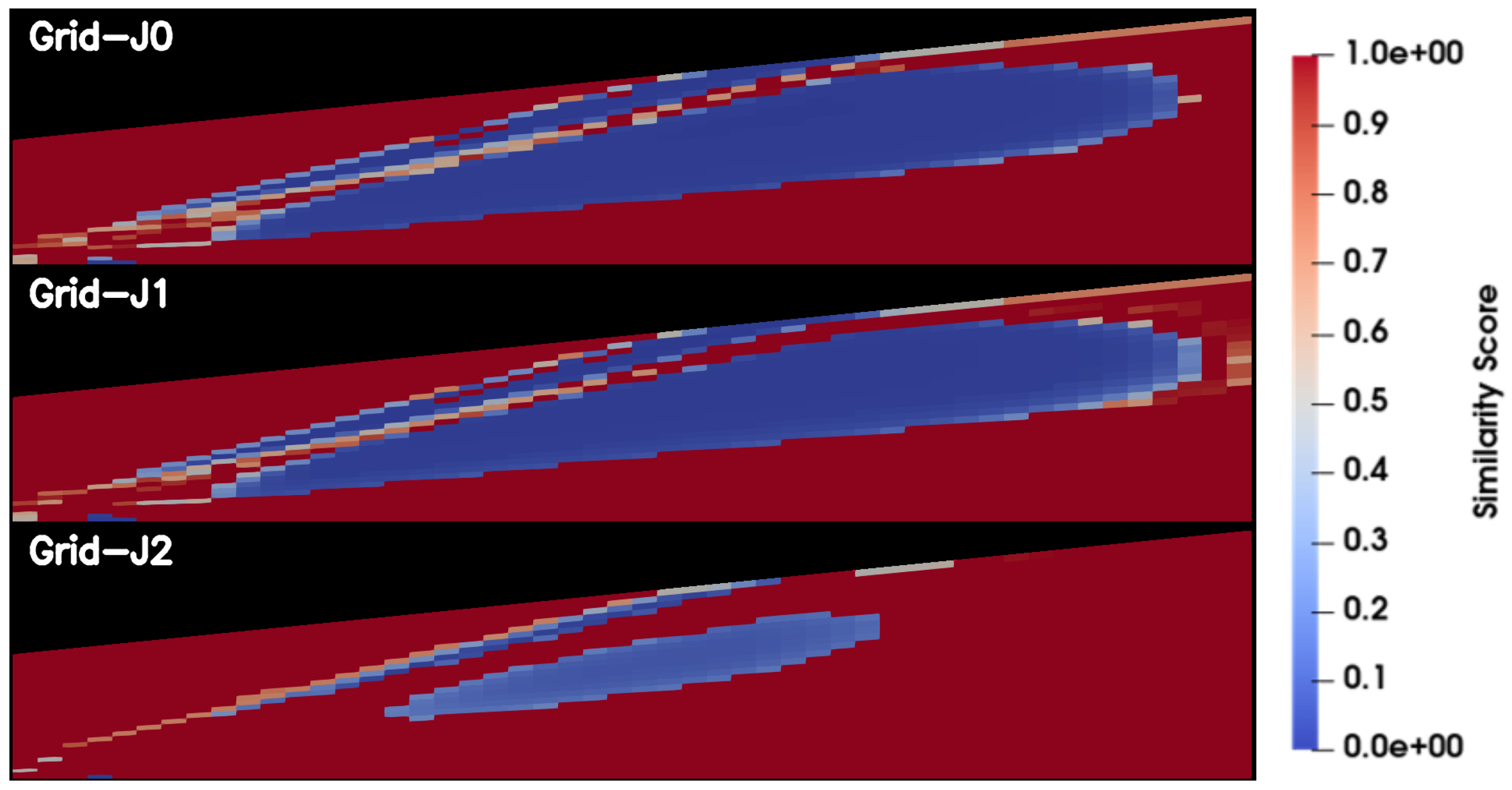
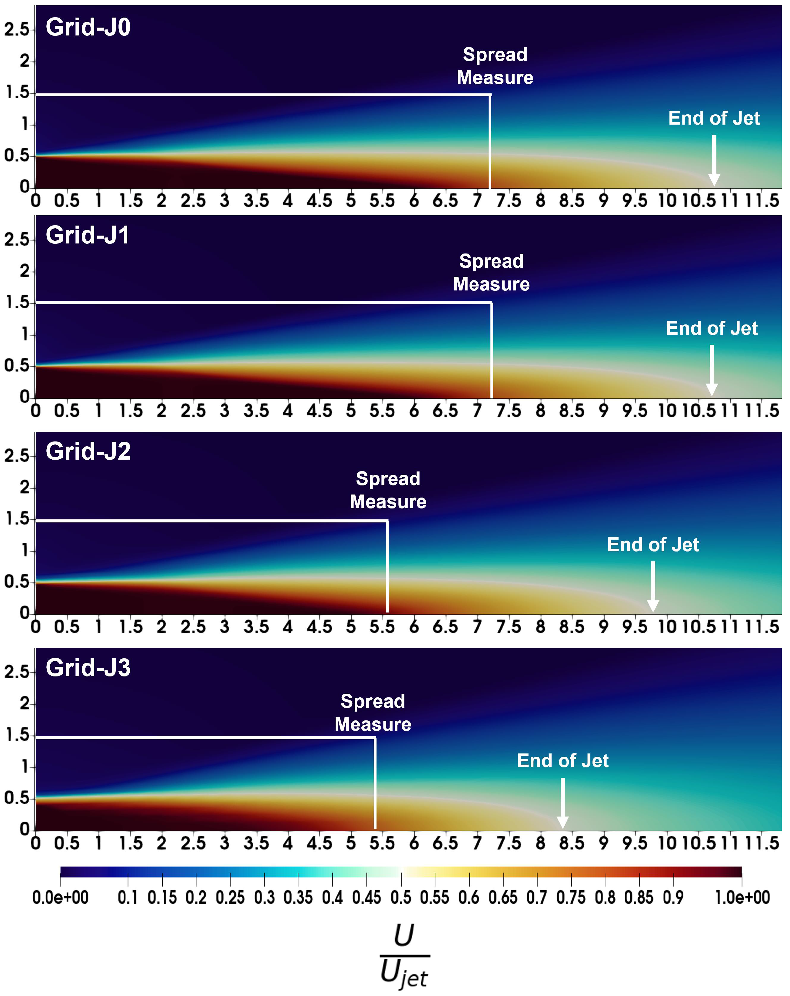
Continuing to Figure 30, Figure 31 and Figure 32, where the individual velocity gradients $\partial U_0/\partial x_0$ and $\partial U_0/\partial x_1$, as well as their combined set $\partial U_0/\partial x_0,,\partial U_0/\partial x_1$, are used as features, it is evident that none of the gradient-based features capture the mesh differences along the centerline as clearly as the $U_0$ feature. 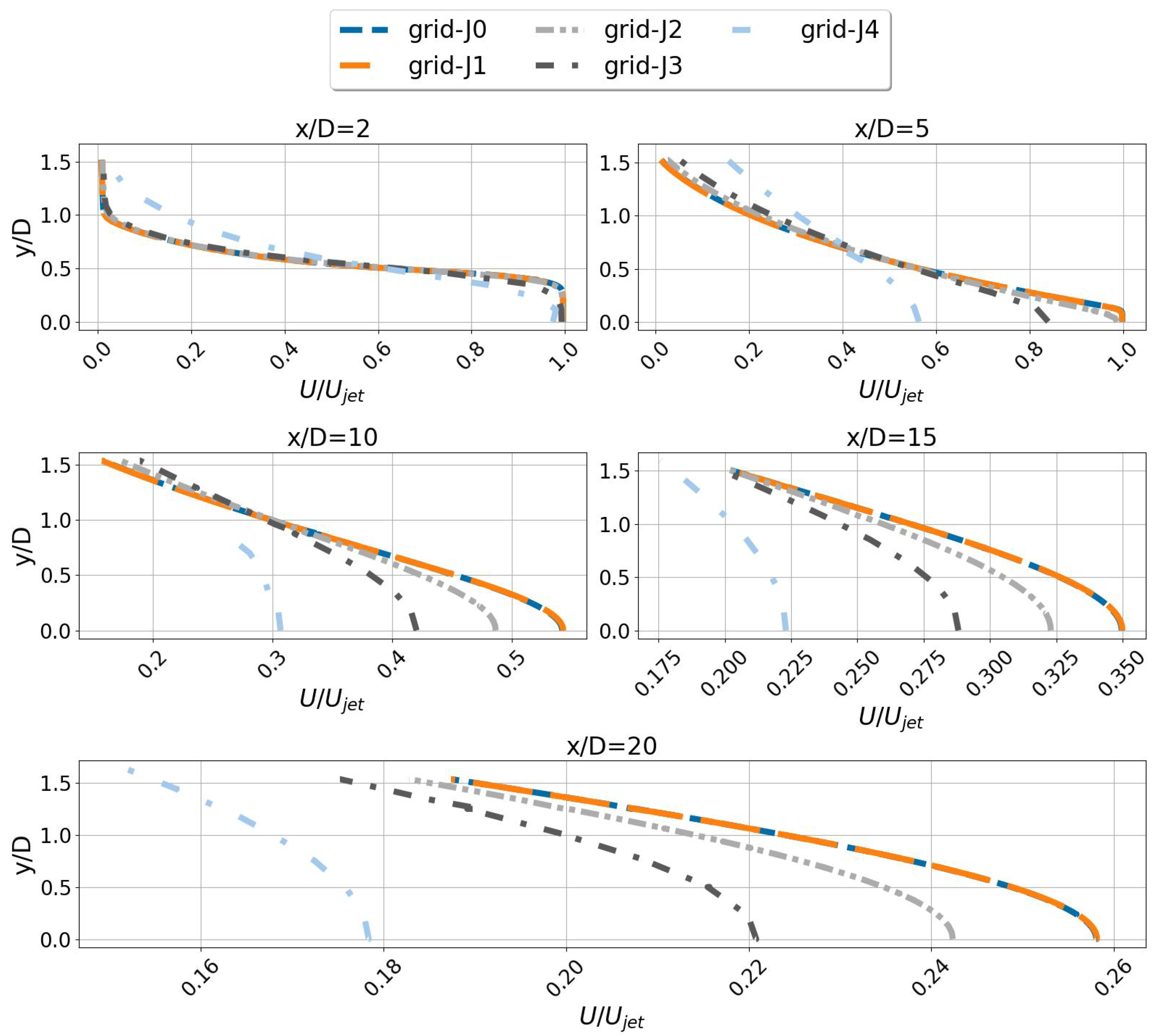The velocity profiles in Figure 33 help explain this behavior. From Figure 33, it can be observed that the refinement of the mesh extends the jets’ influence down the domain, as noted by the “End of Jet” annotations. The refinement also slows the spread of the jet in the radial direction as marked by the “Spread Measure” annotation, which was placed at y = 1.5 and extended until $U/U_{jet}=0.05$. When comparing these profiles to the similarity fields generated using $\partial U_0/\partial x_0$, the model primarily detects changes in the region where the jet spreads outward, approaching the freestream value. The $U_0$ feature detects the differences along the center line of the jet. Finally, the $\partial U_0/\partial x_1$ feature shows minimal variation between the meshes, except in the immediate vicinity of the jet inlet. The combined-gradient feature set produces a similarity field that emphasizes many of the same regions identified by the individual gradients. Importantly, as the combined result is not a linear superposition of the two single-feature outputs, but it resembles the $\partial U_0/\partial x_0$ prediction while incorporating some of the lowest similarity regions associated with $\partial U_0/\partial x_1$, these trends suggest that the model assigns greater influence to the more informative gradient component.

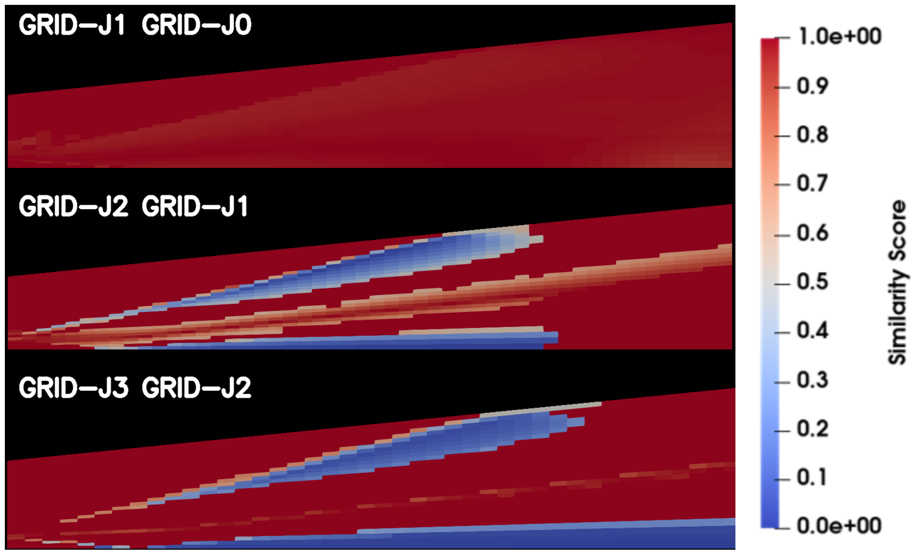
To better assess how each feature performs across the full grid hierarchy, Figure 34 and Figure 35 present the similarity scores for each sequential grid pair, (J3, J2), (J2, J1), and (J1, J0), in the jet flow case, using the $U_0$ feature and the combined gradient features $\partial U_0/\partial x_0$ and $\partial U_0/\partial x_1$. Both feature sets correctly indicate that there is essentially no change in the solution between grids J1 and J0, consistent with the mesh-confirmation analysis. The differences between the feature sets become more apparent when comparing grids J2 and J1. The $U_0$ feature suggests that the change between J2 and J1 is larger than the change between J3 and J2. This trend is physically reasonable when considering the relative refinement ratios: J2 to J1 has a refinement ratio of 2.6, whereas J3 to J2 has a refinement ratio of 1.7. The larger refinement jump between J2 and J1 naturally allows for more substantial differences to emerge in the computed solution.

When comparing the results from the gradient feature sets $\partial U_0/\partial x_0$ and $\partial U_0/\partial x_1$ to the $U_0$ feature, we observe that the gradient-based features do not reproduce the same trend in which the change between grids J2 and J1 exceeds that between J3 and J2. Another noteworthy observation is that, for both gradient features, the regions highlighted with low similarity scores remain consistent across all grid pairs. In other words, the areas identified as changing do not significantly shift in shape or location as the mesh is refined. This behavior further supports the reliability of the model, given that the jet meshes were generated using a uniform global refinement ratio applied to all cells. Because no localized refinement was introduced, any meshing deficiencies are addressed uniformly as the grid is refined. As a result, one would expect the regions of physical change in the solution to remain in the same locations while their magnitude evolves with each refinement step—a trend that is reflected in the similarity predictions.

5.4. Summary Observations: Feature-Set Sensitivity and Comparative Performance

From the analysis of both cases, no single feature set emerged as the clear best choice. Each feature set produced results that were logical and consistent with the physics. The $U_1$ velocity was the least informative. It showed very little difference between grids in either the jet or bump cases. The $U_0$ velocity performed better. In the bump case, it highlighted changes near the bump and in the near-wall wake region. In the jet case, $U_0$ captured large differences along the centerline, which agrees with the mesh-confirmation findings.

The gradient features were the most sensitive. For the bump case, they produced the lowest similarity scores and exposed questionable gradient behavior in the coarse meshes. For the jet case, the $\partial U_0/\partial x_0$ gradient dominated, while $\partial U_0/\partial x_1$ showed almost no meaningful distinction between grids. It is also important to note that combining the two gradient features did not create a linear combination of their individual outputs. Instead, the combined set produced a new pattern influenced by both, but weighted more strongly toward $\partial U_0/\partial x_0$.

Overall, there was no clear best feature set for the jet case. Both velocity and gradient features had strengths and weaknesses. The model performred well with either a single feature or multiple features. There is also potential value in using other flow variables, such as pressure or turbulence quantities, but additional work is needed to confirm their effectiveness. Second-order gradients were also tested, but they did not offer noticeable improvements over the first-order features, and hence, for brevity, were not included in this paper.

Based on these results, the authors recommend following the “No Free Lunch” theorem of machine learning [38]. This principle states that no single model, or in this context, no single feature set, works best for all problems. Each application requires testing and selecting the feature set that performs best for that specific case. For practical use of this model, two suggestions are made. First, we suggest starting with both velocity ($U_0$, $U_1$) and gradient feature sets ($\partial U_0/\partial x_0$, $\partial U_0/\partial x_1$), then placing greater emphasis on whichever feature set aligns most closely with the needs and physics of the user’s problem. Second, the user is advised to not “boil the ocean” with feature selection. If too many features are added to the model, its prediction ability and interpretability will be impaired. This is due to the “curse of dimensionality” [39], which describes how finding structures becomes more difficult when the dimensionality of the data is higher. For clustering approaches, this is caused by the increase in distance between points making the data to become more sparse, making the cluster fitting process less effective at extracting meaningful groupings. In addition to reducing the model’s effectiveness, it also hinders the user’s ability to interpret the decision-making of the model, as the user cannot as easily link the similarity score values to any particular input feature. Currently, the authors advise keeping the number of features below 5, as this was the maximum tested during development.

5.5. Computational Cost

Table 6. Computational benchmark of simulation time for the CFD cases.

Case	Iterations	Mesh Resolution	Time (s)
2D Bump in Channel	10,000	B0	990
		B1	425
		B2	225
		B3	215
		B4	185
Turbulent Flat Plate	5000	F0	3450
		F1	1650
		F2	1200
		F3	1050
		F4	1000
Free Jet Flow	2000	J0	675
		J1	500
		J2	90
		J3	65
		J4	50

shows a benchmark of the computational resources and time used to calculate the CFD solution. In each case, 8 cores were used along with OpenFOAM’s hierarchical decomposition method, with all decompositions being placed in the streamwise direction.

Benchmarking of the ML method was then performed using 8 cores, and was performed by monitoring the full ML pipeline from cell creation to final similarity score prediction. The results of the benchmarking are summarized in

Table 7. Computational benchmark of time taken to calculate the ML model similarity scores.

Case	Ram Consumption (GB)	Total Data Size (Rows)	Time (s)
2D Bump in Channel	1.5	220,150	80
Turbulent Flat Plate	3.0	818,400	335
Free Jet Flow	1.5	241,000	95

. Comparing the ML results to the CFD computation time is minor compared to the CFD calculation time, with most of the cases taking less than half the time of the calculation of the finest CFD solution. The RAM usage of the workstation was seen to increase with the increasing mesh size (expressed by “Total Data Size” in the table), but not at a rate that was prohibitive when running on less powerful machines.

5.6. Summary Observations: Model Usage Recommendations

Throughout the two case studies, a few general observations about the usage of the model can be made. The first is that the model is not an automated replacement for mesh convergence analysis but instead a decision-making aid. The case studies highlight that the model solution is dependent on many choices made by the user, particularly feature selection, normalization, and parent mesh resolution. It is important to understand that just because a case is considered converged according to one set of features, that does not mean it is converged with respect to all features. This tool should be used to prompt the user to explore differences in results to better understand the underlying dissimilarities in the flow field that are causing the answers. The second observation is that the tool is not a replacement for more automated algorithms like AMR, but instead a post-hoc tool to be used alongside them in the development process. The similarity metric, while intuitive, does not provide an actionable number for how much refinement is required to reach mesh convergence. This makes the tool much more suitable as an aid to focus the user’s attention on areas of the mesh that need investigation.

5.7. Possible Future Work

Building on the results presented in this study, several extensions of the methodology appear promising and warrant further investigation, and the authors intend to include these in future publications:

• 3D implementation. The current approach should be tested on fully 3D geometries. Such an extension will help evaluate the method’s robustness and identify any computational optimizations needed to handle the substantially larger data sets typical of 3D simulations.
• Enhanced feature construction. Future work could explore more advanced feature formulation techniques that encode spatial distribution information within each cell set. Such features may allow the model to better detect complex flow behavior, for example, when recirculation zones shift or change direction between grid refinements.
• Improved cell–set generation strategies. In this study, cell sets were generated using only a coarse parent mesh. Alternative strategies, such as cell sets aligned with boundary-layer prism layers or regions of expected high gradients, may offer improved localization and better highlight regions of greatest interest to the user.
• Explainability for ML predictions. Incorporating explainability tools into the ML framework would provide users with deeper insight into the rationale behind the assigned similarity scores. Such tools would strengthen user confidence and support more informed decision-making when interpreting the effects of mesh modifications.

6. Conclusions

This work introduced a machine-learning-based framework designed to improve mesh generation and mesh evaluation by providing users with localized, visually intuitive feedback on how mesh changes affect the underlying flow solution. Unlike prior global error indicators, the proposed method regionalizes model predictions through the construction of “cell sets” derived from a coarse parent mesh. These localized regions serve as the basis for an unsupervised clustering model that compares feature distributions between two grids. A new similarity metric was developed to translate the raw clustering assignments into a continuous scale from zero to one, enabling an interpretable and quantitative measure of local mesh similarity.

The methodology was evaluated using three canonical CFD cases, viz. the turbulent flat plate, the 2D bump in channel, and the axisymmetric jet. These cases are simulated in OpenFOAM across multiple grid levels. Numerical experiments were performed to assess both feature validity and feature selection. The principal findings of this study are summarized as follows.

• The use of coarse mesh-based cell sets proved to be an effective strategy for geographic localization of ML predictions. Future work is needed to automate this process further to reduce user input.
• The similarity metric reliably produced values that were logically consistent with clustering behavior and exhibited expected trends across grid refinements.
• Although the model is unsupervised, it was observed that user input is necessary to define what constitutes a meaningful change between grids. Without such input, the model is overly sensitive and may assign low similarity scores to regions where the distribution changes but the magnitude change is insignificant.
• The ML predictions aligned well with traditional mesh convergence behavior. The model provided feedback that agreed with physical intuition, highlighted regions where mesh differences were expected, and maintained stable predictions across grids with modest refinement differences.
• The feature selection study showed that the model can sensibly process multiple flow features, but that no single feature set is universally superior. The most appropriate feature set is problem-dependent and should reflect the aspects of the flow that are most important to the user.

Taken together, these findings demonstrate the potential of ML-informed similarity assessments to augment traditional mesh evaluation techniques. The approach offers a practical and physics-consistent way to identify where mesh refinement matters most and to guide mesh design strategies in a more informed and interpretable manner.