Abstract
We studied the hemodynamics of abdominal aortic aneurysms (AAAs) by combining laboratory experiments and numerical simulations, with a focus on potential rupture mechanisms. In particular, we investigated the influence of geometrical features—beyond the commonly used maximum diameter—on flow patterns and the wall shear stress (WSS) distribution. Following our previous in vitro study performed utilizing a symmetrical bulge, we extended the analysis to an asymmetrical aneurysm geometry. Experiments and simulations were conducted under steady flow conditions while varying the Reynolds number over a wide range (490 < Re < 3930), to replicate the flow regimes occurring throughout the cardiac cycle. High-resolution, two-dimensional velocity fields were measured in the lab via image analysis and numerically computed using ANSYS Fluent®. These data enabled a detailed characterization of both flow patterns and WSS distributions in healthy aorta and within the aneurysmal region. The good agreement between numerical and experimental results, as well as consistency with the literature, validates the adopted approach and supports its use for future investigations into AAA hemodynamics and rupture risk assessment.
1. Introduction
Abdominal aortic aneurysm (AAA) is a local irreversible dilatation of the abdominal aorta that usually forms between the renal arteries and the iliac bifurcation; it manifests as a pathological condition that may remain silent, i.e., asymptomatic, unless its sudden rupture happens. This event is associated with a high mortality rate; indeed, it is classified as one of the most leading causes of death in the US [1] and, in general, in the world. Risk factors associated with the formation and the progression of AAAs include advanced age, male gender, Caucasian race, positive family history, smoking, obesity, presence of other large vessel aneurysms, atherosclerosis, hypertension, and further cardiovascular diseases [1,2]. After the diagnosis of AAAs and according to the actual guidelines [3], clinicians evaluate if surgical repair is needed to prevent its rupture; the decision is made after comparing the risk of rupture with the risk associated with the repairing itself. The recommendation in this sense is based on a geometrical constraint, i.e., a limit threshold on the maximum diameter of 5 cm for women and of 5.5 cm for men. Nevertheless, the literature reported of both dilation exceeding the limit threshold and remaining unruptured as well as of ruptured AAAs smaller than it [4,5]. Indeed, several more geometrical/morphological, mechanical, and hydrodynamical variables have proven to strongly impact aneurysm evolution and are being analyzed to focus on how they may correlate with rupture and, eventually, help in the clinical management of the disease. Among them, we highlight the following: aspect ratios; wall surface area; volume, symmetry, tortuosity, curvature, and wall thickness; compactness, wall shear stress (WSS) distribution including time-averaged (TWSS) and peak (PWSS) values; oscillatory shear index (OSI); intraluminal thrombus (ILT) thickness; relative residence time (RRT); vorticity; and turbulence intensity [6,7,8,9,10]. Both numerical and experimental (in vivo and in vitro) models demonstrate fundamental tools to assess the variation and the mutual interactions between these quantities. A recent article reviewed the latest advances in computational analysis on AAAs [1], and widely described there and in the references therein [5,7,11], the considered numerical schemes that are based on the solution of the Navier–Stokes equation in a linear conduit with varying geometry using self-developed or commercial software and the level of complexity that is related to the definition of the inlet flow, of the geometry, and of the fluid-structure interactions [12]. In vitro modeling represents a consolidated methodology suitable for reproducing the cardiovascular system within a strictly controlled setting, both in physiological and pathological conditions; also, they represent a reliable tool for validating numerical methods and outcomes [13,14,15,16]. In this regard, the implementation of patient-specific modeling built using clinical data obtained through medical imaging is of particular relevance as it allows for increasing the accuracy of both the anatomical/geometrical and the hemodynamical aspects of system [17,18]. Moreover, the integration of classical approaches, as computational fluid dynamics (CFD) and in vitro models, and deep learning, represents the cutting-edge approach of the current research [4,19]. This paper is in continuity with [20] in which we considered a simplified laboratory model of a symmetric AAA; indeed, here we performed a new laboratory measurements’ campaign using an asymmetric geometry of the sac. For both cases, we coupled the experiments with a numerical study of a simplified model of AAAs with rigid walls performed using the commercial software ANSYS Fluent® (Ansys 2022 R2). Simulations were run in steady flow conditions and varying the Reynolds number in the range 490 < Re < 3930. The assumption of Newtonian flow behavior and of vessel rigid walls adopted here appears to be coherent with the literature even if more accurate models should imply a different rheology behavior and walls deformation (see [19] and reference therein). The 2D description of the experimental flow field was obtained using image analysis. Here, we considered Hybrid Lagrangian particle tracking, HLPT [21], a technique suitable at providing output of both the particles’ trajectories and the velocity fields (instantaneous and time-averaged) on a regular grid. Based on the analysis of the velocity fields and by comparing the experimental results with the numerical predictions, we were able to investigate the evolution of flow patterns and the distribution of the WSS as functions of the imposed flow regime and geometric asymmetry. These findings may support the identification of clinical scenarios suitable for investigating the correlation between aneurysm-induced wall shear stress (WSS) distribution and rupture risk. Furthermore, with this study, we aimed to validate the scheme built in simplified conditions in order to consolidate the procedure in preparation of its future application in more complex and realistic conditions.
The paper is organized as follows: Section 2 includes the description of the experimental model and of the measuring technique as well as of the numerical scheme considered; in Section 3, we show and comment on the obtained results, and in Section 4, we provide the main conclusions and some ideas for future work.
2. Materials and Methods
2.1. Experimental Investigation Setup
The main features of the experimental facility employed for the investigation will be provided herein. For a more detailed description, refer to [20]. The fluid circulated within the system was pure water provided by a reservoir equipped with an overflow outlet to remove water exceeding a set level; this ensures a constant flow rate Q within the hydraulic circuit. Using water in the model, we implicitly assumed that the blood behaves as a Newtonian fluid; this assumption is consistent with the phenomena under study being a vessel transverse size greater than 1 mm [15]. Indeed, this assumption is reasonable for systemic circulation, given the average dimension of blood cells, ~10−3 cm. However, a non-Newtonian rheology is well suited for modeling small arteries or stenoses [12]. The fluid moved from the upstream tank through a custom-made Pyrex glass tube mimicking both a healthy aorta (straight portion) and the AAA, designed with symmetrical or asymmetrical bulges, depending on the case under investigation, hereinafter SYM and ASYM cases (see Figure 1). The total length of tube for the SYM model was 1.060 m with a diameter ranging from d = 0.018 m in the straight portion to a maximum bulge diameter of D = 0.030 m and a sac length of La = 0.060 m (dilatation ratio D/d = 1.66, elongation ratio La/d = 3.33). The ASYM model was 1.300 m long, with the same diameter in the straight portion (d = 0.018 m), maximum enlargement diameter D = 0.025 m, and a sac length La = 0.080 m (dilatation ratio D/d = 1.66, elongation ratio La/d = 4.44). We estimated the asymmetry ratio β = r/R [5], where r and R are the distances of the posterior and anterior walls from the aneurysms’ axis measured in correspondence to the sac maximum enlargement section. The corresponding values were 0.6 (ASYM) and 1 (SYM), respectively. To fulfill geometric similarity in both cases, we considered the physiological shape of the bulge model with a 1:1 scale. Moreover, the geometry of the model was representative of an aneurysm at a consolidated stage of the disease (i.e., increase in diameter > 50%).
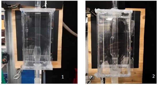
Figure 1.
Pyrex glass tubes with (1) symmetrical or (2) asymmetrical bulges.
The test section was enclosed in a rectangular plexiglass container (10 × 10 × 25 × 10−6 m3), filled with the same fluid flowing through the circuit, to minimize light refraction between air and water and to allow for consistent optical measurements. Out of the bulge, the water flowed through a flowmeter which provided the flow rate. To visualize particle trajectories and reconstruct the fluid mean velocity field in the test section, the passive tracer VESTOSINT® 2157 natural (polyamide 12) was introduced. The tracer’s mean particle diameter (~56 µm) and density (1016 kg/m3) enabled it to passively follow the fluid motion. A green laser (5 W diode, 532 nm wavelength) illuminated the test section, generating a light sheet in the (x, z) plane, where the z-axis was vertical, and the x-axis was horizontal and orthogonal to the camera acquisition axis. It is worth noting that the light sheet thickness was sufficiently limited to minimize the out-of-plane velocity component. Images for each run were captured using a high-resolution Mikrotron EoSens camera (1280 × 1024 pixels) equipped with a 50 mm lens. Before the recording, the camera was positioned frontally to the test section, ensuring its acquisition axis was orthogonal to the measurement area. To capture a larger portion of the tube, the camera was rotated 90°, secured on a tripod, and placed at a distance that allowed for proper framing and focusing. Multiple recordings for different flow rates were carried out at 400 frames per second, each lasting about 60 s. The Core Express® digital recording system, managed via a PC, controlled image acquisition and storage. Hybrid Lagrangian Particle Tracking (HLPT) was used to elaborate the acquired images. The 2D tracking approach relies on solving the optical flow equation, which identifies regions in each image with high gradients in light intensity [21]. These regions can be linked to tracer particles, making them suitable features to track in the sequence. After the identification of the features, the method reconstructs the trajectories. The displacement along the trajectory and the associated elapsed time are then used to evaluate the particle velocity, and the fluid motion is then characterized in a Lagrangian reference frame. Sparse velocity vectors are then regularized along a grid of square meshes overlapped to the area of interest. Time-averaged horizontal and vertical velocity components (U, ) are computed for each grid mesh providing the Eulerian description of the flow field. The velocity fields are then post-processed to compute all the quantities of interest for the description of the fluid motion. In Table 1 the experimental parameters corresponding to the performed experiments are listed.

Table 1.
Experimental parameters in the performed experiments: flow rate Q, Reynolds number Re, bulk velocity Wb, and WSS assuming a Poiseuille velocity profile (τPois).
2.2. Numerical Investigation Setup
For both the SYM and ASYM bulges, numerical simulations were performed using the commercial software ANSYS Fluent®. The discretization of the domain was performed via the software provided by ANSYS (Fluent Meshing), which guarantees the generation of a simply connected domain (Watertight Geometry). The 3D drawings of both SYM and ASYM bulges were realized with AutoCAD® (2022 by Autodesk), starting from pictures of the physical models with their dimensions. These drawings were imported in the ‘Geometry’ component section of Fluent. Figure 2 reports the pictures of the AAA models. The computational domain was discretized using a hybrid mesh of poly-hexcore elements comprising 5 layers of polyhedral elements close to the boundaries and hexahedral (hex) elements in the core region. This discretization method uses polyhedral elements close to boundaries to maintain accuracy in complex geometries and for a better simulation of the boundary layer while utilizing the efficiency of hex elements in the bulk flow.
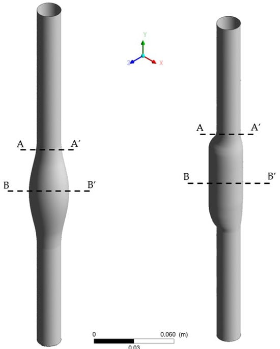
Figure 2.
3D drawing of the SYM (left) and ASYM (right) model of AAA; sections (A-A’) and (B-B’) indicate the proximal neck and the midplane of the aneurysm sac, respectively.
To assess mesh independence, simulations were performed using three refinement levels: a coarse mesh (maximum element size = 0.005 m), a medium mesh (5× finer than coarse), and a fine mesh (2× finer than medium) while holding constant all other settings, including boundary conditions, solver parameters, and turbulence models. It is worth noting that for all cases, while a nominal maximum element size was imposed, the meshing algorithm dynamically adjusted local element sizes to conform to geometric curvature (e.g., near the AAA wall) and satisfy skewness/quality criteria. Consequently, the realized maximum element size was smaller than the target value in all cases, as confirmed by post-processing.
The centerline velocity in the region of the unhealthy flow profile (where the maximum velocity occurs within the AAA) was selected as the key metric for convergence analysis due to its sensitivity to mesh resolution and its relevance to hemodynamic characterization in AAAs.
The relative difference between successive meshes was quantified as follows:
where ϕ represents the centerline velocity. A difference of <1% was predefined as the threshold for mesh independence. The differences were 2.5% (coarse-to-medium) and 0.1% (medium-to-fine), indicating that the medium mesh achieved sufficient accuracy for further simulations.
Table 2 shows the main features of the discretization adopted after the mesh optimization procedure. The minimum and maximum size of the grids and the total number of elements are provided. Note that the greater number of meshes that characterizes the ASYM model, with minimum and maximum sizes comparable between the two models, is related to its geometry which requires a greater number of meshes for accurate characterization.
Table 2.
Main features of the grids employed for both models.
When simulating pipe flow in CFD, the choice of inlet boundary condition is critical, particularly when comparing laminar and turbulent regimes. The inlet boundary condition for both models is ‘Velocity inlet’, setting a Poiseuille-law velocity profile for which an average velocity value equal to the ratio of the fluid flow rate to the cross-sectional area is used (see Wb values in Table 1). A velocity profile à la Poiseuille was also adopted for cases #5 and #6, which are characterized by a transitional or turbulent flow regime. For laminar flow, the Poiseuille profile is appropriate because it represents the exact analytical solution for fully developed flow. In contrast, turbulent flows exhibit a flatter velocity profile due to enhanced momentum mixing. However, to ensure consistent comparisons across different geometries and flow conditions, we standardized the inlet boundary condition using the Poiseuille profile—despite its inaccuracy for turbulent cases—as a controlled simplification. This approach isolates the effects of geometry and flow rate without introducing additional variability from differing inlet profiles. The ‘pressure outlet’ boundary condition was set at the outlet surface. The ‘Wall’ boundary condition was assigned to the wall. The ‘no-slip’ condition was set which prescribes the fluid to adhere to the interface with the wall and move with the same velocity at zero velocity in our models since the walls were fixed. The viscous model adopted for cases #1–4, with Re ranging from 490 to 1970, was the laminar one. For cases #5 and #6, given the remarkable robustness and reliability in simulations involving similar geometries and Re within the intermittency region, the k-ω SST turbulence model was chosen to close the Reynolds-Averaged Navier–Stokes equations (RANS).
Numerical Model Validation
To validate the numerical model, we considered the SYM scheme and compared the experimental outcomes shown in [20] with their numerical counterpart obtained with the simulations. In Figure 3, we show run#2: the experimental (E), numerical (N), and the Poiseuille velocity profiles calculated (a) in the inflow zone just above the proximal neck (A-A’), and (b) in the midplane of the aneurysm sac (B-B’); (c) the distribution of the normalized WSS in the vessel calculated as the product of the spatial gradient of the velocity component normal to the wall with the fluid viscosity (for the ASYM profile, the posterior wall is considered). Normalization of the shear stress τ was performed dividing it by the value of the WSS recovered in correspondence of the healthy aorta.
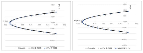
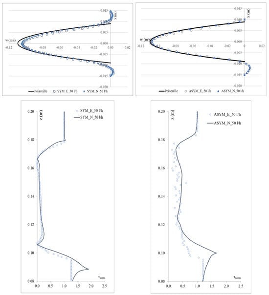
Figure 3.
Experimental (E) and numerical (N) axial velocity profiles obtained for SYM (left) and ASYM (right) models in run#2, in the inflow zone A-A’ (top), and in the center of the aneurysm sac B-B’ (center); Normalized WSS (bottom). The black continuous line plotted with the velocity profiles is the Poiseuille law. Flow is from top to bottom.
To quantitatively assess the similarity between the numerical and the experimental profiles for each quantity of interest, i.e., the axial velocity in the inflow zone and in the center of the aneurysm and the Normalized WSS, the Root Mean Square Error (RMSE) was employed. The RMSE is defined as the square root of the mean squared differences between corresponding data points in the two plots, calculated as
Here, y1,i and y2,i denote the i-th points of the first and second datasets, respectively, and N is the total number of points. The RMSE reflects the average magnitude of discrepancies, with values closer to zero indicating higher agreement. To make the error metric relative to the range of the observed data, the RMSE is normalized by dividing it by the difference between the maximum and minimum observed discrepancy and multiplying by 100, resulting in the NRMSE. This normalization allows for easier comparison across different datasets or models with varying scales.
The NRMSE values for axial velocity in the inflow zone were 0.05% (SYM) and 0.15% (ASYM), while in the aneurysm center, they were 0.11% (SYM) and 0.17% (ASYM). For Normalized WSS, the NRMSE values were 3.10% (SYM) and 4.25% (ASYM). The agreement we found appeared quite good and allowed us to consider both the models with the selected closure scheme as suitable for the subsequent analyses.
3. Results and Discussion
In this section we show the experimental and numerical results obtained in both SYM and ASYM configurations varying the flowrate, i.e., the Reynolds number, as indicated in Table 1.
3.1. Flow Patterns in ASYM AAA
In Figure 4, we show the streamlines and the colormaps of the average longitudinal velocity field measured in the ASYM experiments performed at different Re. The flow appears as a jet flow forming at the inlet of the aneurysm which separates in correspondence of the proximal neck into a recirculating zone and reattaches at the outlet nearby the distal neck. The formation of recirculating flow regions in the sac enlargement, already observed in our previous experimental campaign focused on the symmetrical aneurysm shape (see plots in ref. [20]), agrees with the literature [5].
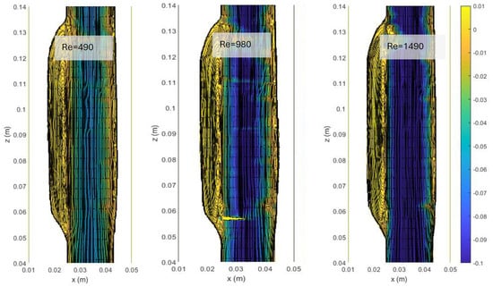
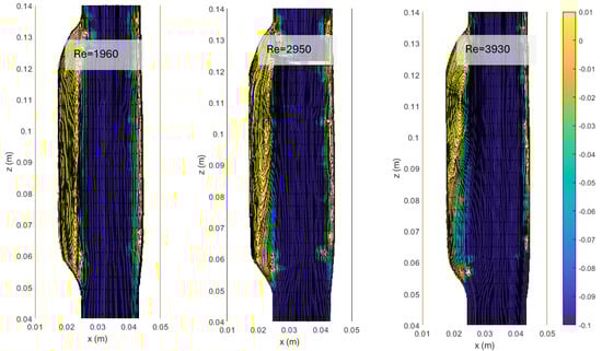
Figure 4.
Streamlines and colormaps of the average longitudinal velocity field measured in the ASYM experiments performed at different Re (Table 2). Flow is from top to bottom.
The images clearly indicate an upward displacement of the vortical structure forming in correspondence of the cavity, which is found to increase with Re. Also, the corresponding increase of turbulence phenomena induces the onset of flow instabilities and nonlinear interactions leading to a modification of the geometrical features of the recirculation zone.
3.2. Numerical Simulations
Based on the validation described above, we ran the numerical simulations for all the considered Re and both the models.
SYM vs. ASYM AAA
- Axial velocity profiles
In Figure 5, we show the axial velocity profiles obtained for SYM and ASYM models in correspondence of the inflow zone and of the center of the aneurysm sac. As expected, the profiles obtained in the healthy aorta for the higher value of the flow rate tend to differ from the theoretical ones. Further, for the higher Re, the structures in the recirculating region tend to feature higher velocity values. This effect is particularly relevant in the ASYM model.
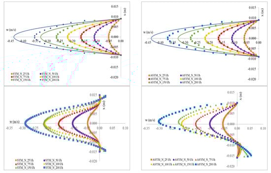
Figure 5.
Axial velocity profiles obtained for SYM (left) and ASYM (right) models in the inflow zone A-A’ (top), in the center of the aneurysm sac B-B’ (bottom). The continuous lines in the upper panels correspond to the Poiseuille theoretical profile.
- WSS Analysis
In Figure 6, we show the WSS calculated for SYM and ASYM models in run#1; the vessel boundaries were also plotted. The profiles indicate low WSS values in the stagnation zone showing two local minima in correspondence of the detachment/reattachment points while two local WSS maxima were recovered nearby the proximal (τP) and the distal (τD) necks; in particular, when the flow regime is laminar, τP were found of the same order of those measured in healthy aorta and the difference increased with Re. The highest values were found out of the aneurysm sac (τD). This behavior is clearly shown in the WSS contour maps represented in Figure 7. From the profiles, we were able to estimate the WSS extrema τD and τP and the average WSS in the sac (τAS) for both SYM and ASYM models. These values are listed in Table 3 and Table 4, respectively. As for the ASYM case, we reported the outcomes recovered in both the anterior and the posterior walls (see Figure 6). In agreement with the literature [5,7], the WSS peaks intensity increases with the asymmetry and in the ASYM model it is found to be higher in correspondence of the anterior wall [22].
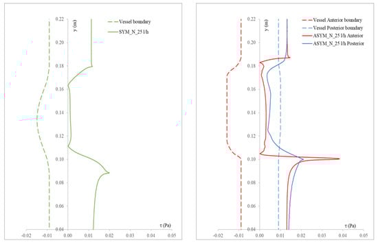
Figure 6.
WSS profiles calculated for SYM (left) and ASYM (right) models in run#1. The dashed lines represent the vessel boundaries. Flow is from top to bottom.
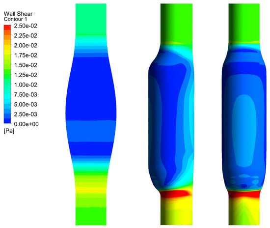
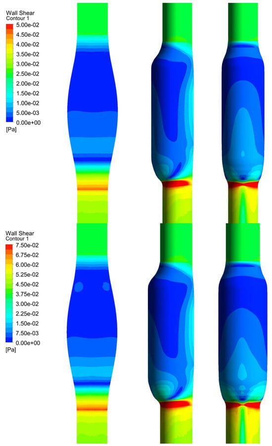
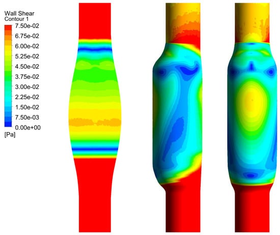
Figure 7.
WSS contour maps calculated for SYM (left) and ASYM (right) models for, from top to bottom, run#1, run#2, run#3, and run#5. Flow is from top to bottom.
Table 3.
WSS maxima in correspondence of the proximal (τP) and distal (τD) necks and in the aneurysm sac (τAS) measured for the SYM model.
Table 4.
WSS maxima in correspondence of the proximal (τP) and distal (τD) necks and the aneurysm sac (τAS) measured for the ASYM model in anterior and posterior walls.
In summary, streamline analysis reveals a flow pattern in the artery characterized by an inlet jet that detaches near the proximal neck, creating stagnation zones, and reattaches close to the distal outlet. The influence of flow regime is evident from both numerical and experimental simulations. Below the turbulent transition threshold in the SYM model, the flow closely approximates the theoretical Poiseuille solution. At higher Reynolds numbers, the flow pattern alters in recirculation zones, with velocities exhibiting a greater average intensity. The WSS is found to vary in a wide range, showing an alternation of high (in correspondence of the proximal and distal necks)−low (inside the aneurysm sac) values; in agreement with the literature [22,23]. The WSS peaks intensity increases with the asymmetry and in the ASYM model it is found to be higher in correspondence of the anterior wall. The complex interplay of morphological, mechanical, and biological factors leading to aneurysm growth and rupture, and/or thrombus deposition is clearly summarized in [19]. We recall that the role of high−low WSS in the aneurysm evolution is still an open issue [23]: on one hand, the recirculating regions characterized by low WSS are associated with increasing OSI and ILT formation, ultimately inducing wall weakening and a possible consequent rupture; on the other hand, high shear stress levels are believed to damage epithelial cells and induce platelet activation, potentially triggering wall failure, coagulation, and thrombus formation.
4. Conclusions
The main goal of this work was to set a procedure based on the integration of laboratory experiments and CFD simulations aimed at a deep investigation of AAAs by focusing, in particular, on the effects of an increase in the inlet fluid velocity and of the bulge shape, symmetry vs. asymmetry. To this aim and based on a previous investigation performed on a symmetric model [20], we consider here an experimental campaign using an asymmetric aneurysm sac. Also, we built a numerical model of both the geometries using the commercial software ANSYS Fluent® and after having validated it, we were able to run the simulations considering the same parameter settings of the experiments.
Even if our model is based on several assumptions, the investigation of the WSS distribution and its correlation with the asymmetry of the sac was found to be in agreement with the literature [22]. Also, the consistency obtained between experimental and numerical results allows one to extend this procedure to flow conditions that we have not considered in this study, i.e., the flow time variation and the compliance of the phantom that will be the object of future research actually in progress. Indeed, both these aspects are related to the WSS time variability: the velocity distribution changes during the cardiac cycle and the compliance, by allowing the wall deformation, acts to modulate PWSS occurring at the systolic peak. Moreover, high to low values transitions appear to play a crucial role in the morphological−mechanical−biological mechanisms inducing aneurysm evolution and thrombus formation as previously discussed [19].
Finally, we remark how a deep comprehension of these complex phenomena necessarily implies a multidisciplinary approach, taking into account a combination of mechanical, fluid dynamical, and physiological aspects.
Author Contributions
Conceptualization, S.E. and M.M.; methodology, S.E. and M.M.; validation, S.E. and M.M.; formal analysis, S.E. and M.M.; investigation, S.E. and M.M.; data curation, S.E. and M.M.; writing—original draft preparation, S.E. and M.M. All authors have read and agreed to the published version of the manuscript.
Funding
This research received no external funding.
Data Availability Statement
The raw data supporting the conclusions of this article will be made available by the authors on request.
Conflicts of Interest
The authors declare no conflicts of interest.
Abbreviations
The following abbreviations are used in this manuscript:
| AAA | Abdominal aortic aneurysm |
| WSS | Wall shear stress |
| TWSS | Time-averaged wall shear stress |
| PWSS | Peak wall shear stress |
| OSI | Oscillatory shear index |
| ILT | Intraluminal thrombus thickness |
| RRT | Relative residence time |
| CFD | Computational fluid dynamics |
| SYM | Symmetrical bulge |
| ASYM | Asymmetrical bulge |
| HLPT | Hybrid Lagrangian Particle Tracking |
| RANS | Reynolds-Averaged Navier–Stokes equations |
References
- Manta, A.; Tzirakis, K. A Comprehensive Review on Computational Analysis, Research Advances, and Major Findings on Abdominal Aortic Aneurysms for the Years 2021 to 2023. Ann. Vasc. Surg. 2025, 110 Pt A, 63–81. [Google Scholar] [CrossRef]
- Chaikof, E.L.; Dalman, R.L.; Eskandari, M.K.; Jackson, B.M.; Lee, W.A.; Mansour, M.A.; Mastracci, T.M.; Mell, M.; Murad, M.H.; Nguyen, L.L.; et al. The Society for Vascular Surgery practice guidelines on the care of patients with an abdominal aortic aneurysm. J. Vasc. Surg. 2018, 67, 2–77. [Google Scholar] [CrossRef] [PubMed]
- Wanhainen, A.; Van Herzeele, I.; Bastos Goncalves, F.; Bellmunt Montoya, S.; Berard, X.; Boyle, J.R.; D’Oria, M.; Prendes, C.F.; Karkos, C.D.; Kazimierczak, A.; et al. Editor’s Choice—European Society for Vascular Surgery (ESVS) 2024 Clinical Practice Guidelines on the Management of Abdominal Aorto-Iliac Artery Aneurysms. Eur. J. Vasc. Endovasc. Surg. 2024, 67, 192–331. [Google Scholar] [CrossRef] [PubMed]
- Chung, T.K.; Gueldner, P.H.; Aloziem, O.U.; Liang, N.L.; Vorp, D.A. An artificial intelligence based abdominal aortic aneurysm prognosis classifier to predict patient outcomes. Sci. Rep. 2024, 14, 3390. [Google Scholar] [CrossRef] [PubMed]
- Belkacemi, D.; Al-Rawi, M.; Abbes, M.T.; Laribi, B. Flow behaviour and wall shear stress derivatives in abdominal aortic aneurysm models: A detailed CFD analysis into asymmetry effect. CFD Lett. 2022, 14, 60–74. [Google Scholar] [CrossRef]
- Urrutia, J.; Roy, A.; Raut, S.S.; Antón, R.; Muluk, S.C.; Finol, E.A. Geometric surrogates of abdominal aortic aneurysm wall mechanics. Med. Eng. Phys. 2018, 59, 43–49. [Google Scholar] [CrossRef]
- Vorp, D.A.; Raghavan, M.L.; Webster, M.W. Mechanical wall stress in abdominal aortic aneurysm: Influence of diameter and asymmetry. J. Vasc. Surg. 1998, 27, 632–639. [Google Scholar] [CrossRef]
- Rawat, D.S.; Pourquie, M.; Poelma, C. Numerical Investigation of Turbulence in Abdominal Aortic Aneurysms. J. Biomech. Eng. 2019, 141, 061001. [Google Scholar] [CrossRef]
- Vergara, C.; Le Van, D.; Quadrio, M.; Formaggia, L.; Domanin, M. Large eddy simulations of blood dynamics in abdominal aortic aneurysms. Med. Eng. Phys. 2017, 47, 38–46. [Google Scholar] [CrossRef]
- Zambrano, B.A.; Gharahi, H.; Lim, C.; Jaberi, F.A.; Lee, W.; Baek, S. Association of intraluminal thrombus, hemodynamic forces, and abdominal aortic aneurysm expansion using longitudinal CT images. Ann. Biomed. Eng. 2016, 44, 1502–1514. [Google Scholar] [CrossRef]
- Saha, S.C.; Francis, I.; Saha, G.; Huang, X.; Molla, M.M. Hemodynamic Insights into Abdominal Aortic Aneurysms: Bridging the Knowledge Gap for Improved Patient Care. Fluids 2024, 9, 50. [Google Scholar] [CrossRef]
- Quarteroni, A.; Manzoni, A.; Vergara, C. The cardiovascular system: Mathematical modelling, numerical algorithms and clinical applications. Acta Numer. 2017, 26, 365–590. [Google Scholar] [CrossRef]
- Deplano, V.; Knapp, Y.; Bertrand, E.; Gaillard, E. Flow behaviour in an asymmetric compliant experimental model for abdominal aortic aneurysm. J. Biomech. 2007, 340, 2406–2413. [Google Scholar] [CrossRef] [PubMed]
- Querzoli, G.; Fortini, S.; Espa, S.; Melchionne, S. A laboratory model of the aortic root flow including the coronary arteries. Exp. Fluids 2016, 57, 134. [Google Scholar] [CrossRef]
- Yazdi, S.G.; Huetter, L.; Docherty, P.D.; Williamson, P.N.; Clucas, D.; Jermy, M.; Geoghegan, P.H. A Novel Fabrication Method for Compliant Silicone Phantoms of Arterial Geometry for Use in Particle Image Velocimetry of Haemodynamics. Appl. Sci. 2019, 9, 3811. [Google Scholar] [CrossRef]
- He, W.; Jiao, M.; Fang, X.; Shen, Z.; Cai, Q.; Zhang, L. In vitro study of flow characteristics in abdominal aortic aneurysm. AIP Adv. 2024, 14, 2158–3226. [Google Scholar] [CrossRef]
- Conlisk, N.; Geers, A.J.; McBride, O.M.; Newby, D.E.; Hoskins, P.R. Patient-specific modelling of abdominal aortic aneurysms: The influence of wall thickness on predicted clinical outcomes. Med. Eng. Phys. 2016, 38, 526–537. [Google Scholar] [CrossRef]
- Bardi, F.; Gasparotti, E.; Vignali, E.; Antonuccio, M.N.; Storto, E.; Avril, S.; Celi, S. A hybrid mock circulatory loop integrated with a LED-PIV system for the investigation of AAA compliant phantoms. Front. Bioeng. Biotechnol. 2024, 12, 1452278. [Google Scholar] [CrossRef]
- Fan, T.; Wang, J.; Wang, X.; Chen, X.; Zhao, D.; Xie, F.; Chen, G. Integrated multidisciplinary approach to aneurysm hemodynamic analysis: Numerical simulation, in Vitro experiment, and deep learning. Front. Bioeng. Biotechnol. 2025, 13, 1602190. [Google Scholar] [CrossRef]
- Espa, S.; Moroni, M.; Boniforti, M.A. In-Vitro Simulation of the Blood Flow in an Axisymmetric Abdominal Aortic Aneurysm. Appl. Sci. 2019, 9, 4560. [Google Scholar] [CrossRef]
- Shindler, L.; Moroni, M.; Cenedese, A. Using optical flow equation for particle detection and velocity prediction in particle tracking. Appl. Math. Comput. 2012, 218, 8684–8694. [Google Scholar] [CrossRef]
- Li, Z.; Kleinstreuer, C. A comparison between different asymmetric abdominal aortic aneurysm morphologies employing computational fluid–structure interaction analysis. Eur. J. Mech. B/Fluids 2007, 26, 615–631. [Google Scholar] [CrossRef]
- Al-Jumaily, A.M.; Embong, A.H.B.; Al-Rawi, M.; Mahadevan, G.; Sugita, S. Aneurysm rupture prediction based on strain energy-CFD modelling. Bioengineering 2023, 10, 1231. [Google Scholar] [CrossRef]


Disclaimer/Publisher’s Note: The statements, opinions and data contained in all publications are solely those of the individual author(s) and contributor(s) and not of MDPI and/or the editor(s). MDPI and/or the editor(s) disclaim responsibility for any injury to people or property resulting from any ideas, methods, instructions or products referred to in the content. |
© 2025 by the authors. Licensee MDPI, Basel, Switzerland. This article is an open access article distributed under the terms and conditions of the Creative Commons Attribution (CC BY) license (https://creativecommons.org/licenses/by/4.0/).