Article

Weakly Nonlinear Instability of a Convective Flow in a Plane Vertical Channel

Institute of Applied Mathematics, Riga Technical University, Zunda Embankment 10, LV 1048 Riga, Latvia
*
Author to whom correspondence should be addressed.
Fluids 2025, 10(5), 111; https://doi.org/10.3390/fluids10050111
Submission received: 10 March 2025 / Revised: 12 April 2025 / Accepted: 19 April 2025 / Published: 26 April 2025

Abstract

:
The weakly nonlinear stability analysis of a convective flow in a planar vertical fluid layer is performed in this paper. The base flow in the vertical direction is generated by internal heat sources distributed within the fluid. The system of Navier–Stokes equations under the Boussinesq approximation and small-Prandtl-number approximation is transformed to one equation containing a stream function. Linear stability calculations with and without a small-Prandtl-number approximation lead to the range of the Prantdl numbers for which the approximation is valid. The method of multiple scales in the neighborhood of the critical point is used to construct amplitude evolution equation for the most unstable mode. It is shown that the amplitude equation is the complex Ginzburg–Landau equation. The coefficients of the equation are expressed in terms of integrals containing the linear stability characteristics and the solutions of three boundary value problems for ordinary differential equations. The results of numerical calculations are presented. The type of bifurcation (supercritical bifurcation) predicted by weakly nonlinear calculations is in agreement with experimental data.

1. Introduction

Convective flows generated by internal heat sources are widespread in nature and engineering. Examples include convection in the Earth’s mantle [1] and the internal heating of liquid blankets of thermonuclear reactors [2]. Convection is one of the factors that has to be taken into account in biomass thermal conversion [3], where heat is released as a result of chemical reactions.
Linear and weakly nonlinear instability theory is often used in applications with the objective to determine when and how a particular base flow becomes unstable [4]. In many cases, instability is undesirable and should be prevented (typical examples of such cases are found in aerodynamics). A different situation takes place in the mathematical modeling of a biomass thermal conversion [5]. In this case, instability leads to more intensive mixing of fluid layers, which, in turn, can lead to a more efficient energy conversion process.
The first step in the stability analysis of a particular base flow is linear stability theory [4]. In a classical hydrodynamic stability theory, a base flow is typically a simple steady one-dimensional flow (such as plane Poiseuille flow), which is obtained analytically as the solution of the equations of motion. Small perturbations are imposed on the flow; the perturbed quantities are substituted into the governing equations and are linearized in the neighborhood of the base flow. Using the method of normal modes, the linearized system of partial differential equations is transformed to an eigenvalue problem for ordinary differential equations where the unknowns are the amplitudes of the normal perturbations, and the eigenvalues are complex wave speeds of the perturbations. This eigenvalue problem is usually solved numerically using spectral methods or the shooting method [6].
Linear stability theory can be used to determine when a particular base flow becomes unstable. This means, in particular, that the parameter describing the system (for example, Grashof number G r ) exceeds the critical value G r c . The development of instability above the threshold is usually analyzed by numerical methods. The solution of the nonlinear system of equations is required at this stage. There are situations, however, where asymptotic analyses may lead to a simplified description of the problem. Assume that the base flow is linearly unstable, but the value of the Grashof number G r is slightly larger than G r c . The growth rate of the most unstable perturbation in accordance with linear stability theory is positive (but very small). Thus, there is hope that the development of instability can be analyzed by the asymptotic expansion of the disturbance amplitude. The evolution of the amplitude of the linearly unstable perturbation can be described by a slowly varying function of time and space variables. The application of the method of multiple scales leads to a nonlinear scalar amplitude evolution equation, which can be solved more efficiently than the full nonlinear system. Such an approach has been effectively used in the past for different flows. Examples include but are not limited to plane Poiseuille flow [7], shallow water flows [8], and rapidly decelerating flows in pipes [9].
In the present paper, we perform linear and weakly nonlinear stability analyses for the case of a convective flow in a plane vertical channel. Convection is induced by internal heat sources distributed within the fluid. We restrict ourselves to the case of small Prandtl numbers. In this case, instability is of a hydrodynamical nature (shear instability [10]) so that the effect of thermal perturbations is small and can be neglected.
The main contributions of the present study are summarized as follows:
  • A weakly nonlinear approach is used in the paper in the limit of small Prandtl numbers to investigate the behavior of the most unstable perturbation. The asymptotic expansion is constructed in the neighborhood of the critical point where the Grashof number is slightly larger than the critical value.
  • The amplitude evolution equation for the most unstable mode is derived from the equations of motion in contrast with many other studies where a phenomenological approach is used (the form of the amplitude equation is assumed without derivation). It is shown that the amplitude evolution equation is the complex Ginzburg–Landau equation (CGLE). The formulas for the calculations of the coefficients of the equation are derived in the paper. It is shown that the coefficients depend on the solutions of the linear stability problem, the corresponding adjoint problem, and three boundary value problems, which are obtained using the expansion procedure.
  • The formulas for the coefficients of the CGLE do not change and are the same for different convective flows between two parallel vertical planes. These flows include (a) flows due to heat sources of constant or variable density; (b) flows due to a temperature difference between the walls of the channel or the superposition of cases (a) and (b). In all these cases, the same CGLE derived in the present paper can be used. The input data for the calculation of the coefficients of the CGLE are as follows: (1) the velocity profile obtained from the solution of the steady state Navier–Stokes equations under the Boussinesq approximation, and (2) the corresponding critical values of the parameters of the linear stability problem.
  • To illustrate the procedure, we perform calculations for the case of heat sources of constant density. The results show that the CGLE correctly predicts the type of bifurcation (supercritical bifurcation) in agreement with experimental data. This means that when the base flow becomes linearly unstable, a new laminar flow with a more complicated structure sets in. In addition, the CGLE also predicts the existence of periodic solutions for some values of the parameters also in agreement with experimental data.

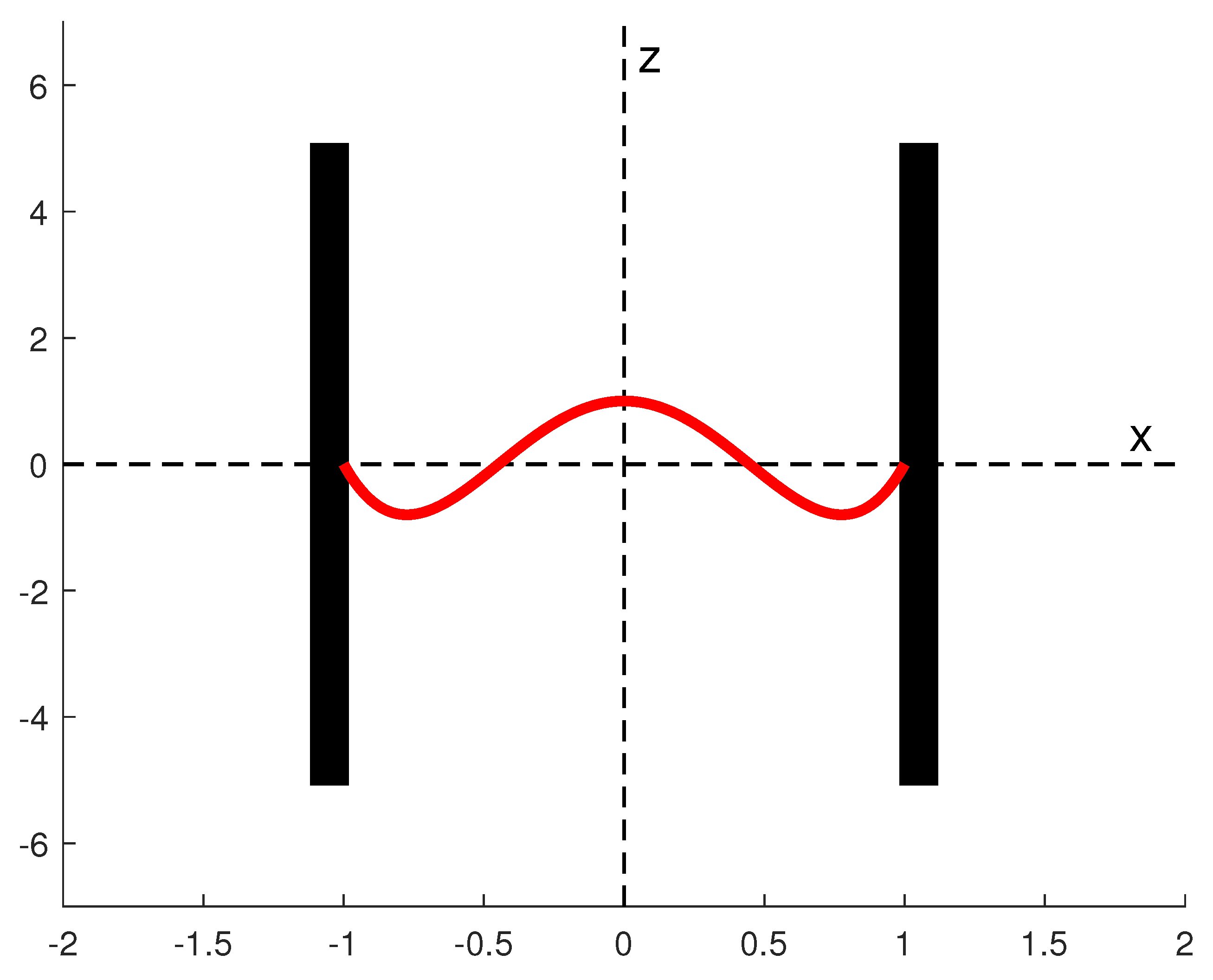
2. Mathematical Formulation of the Problem

Consider a flow of a viscous incompressible fluid in the region D = { h < x ˜ < h , < y ˜ < + , < z ˜ < + } in a plane vertical channel bounded by two infinite parallel planes x ˜ = ± h . We introduce a system of Cartesian coordinates ( x ˜ , y ˜ , z ˜ ) with the origin at the axis of the channel; the z ˜ -axis is directed upwards. It is assumed in sequel that the variables with tildes are dimensional while the variables without tildes are dimensionless. Convection is generated by internal heat sources Q ˜ = Q ˜ ( x ˜ , y ˜ , z ˜ , T ˜ ) distributed within the fluid, where T ˜ is the absolute temperature. Different forms of internal heat sources are considered in the literature: (a) Q ˜ = Q ˜ 0 = c o n s t [10,11,12]; (b) Q ˜ = Q ˜ 0 exp ( a x ˜ ) , where a is a constant [13]; (c) nonlinear heat sources distributed in accordance with Arrhenius’ law [14,15,16]:
Q ˜ = Q ˜ 0 e E / ( R 0 T ˜ ) ,
where E is the activation energy and R 0 is the universal gas constant. Distribution (b) takes place where a light beam is passing through a fluid and the absorbed energy is distributed in the form of heat. Distribution (c) is usually used in case a chemical reaction is taking place in the fluid.
The flow is described by the dimensionless form of the system of the Navier–Stokes equations under the Boussinesq approximation (see [17,18,19,20,21]):
v t + G r ( v · ) v = p + Δ v + T e k ,
T t + G r v · T = 1 P r Δ T + Q P r ,
· v = 0 .
Here, v is the velocity of the fluid, T is the temperature, p is the pressure, and e k = ( 0 , 0 , 1 ) . We assume that Q = Q ( x , T ) .
The analysis of the linear and weakly nonlinear instability of the flow can be performed for different functions Q = Q ( x , T ) . In order to illustrate all the procedures, we choose the case of a constant density of heat sources ( Q = Q 0 ), and all numerical calculations in the paper are performed for this case. The dimensionless form of (2)–(4) is obtained using the following units of measurement: h, h 2 / ν , g β Q 0 h 4 / ( 2 ν κ ) , Q 0 h 2 / ( 2 κ ) , and ρ g β Q 0 h 3 / ( 2 κ ) for the length, time, velocity, temperature, and pressure, respectively. Here, ν is the viscosity, β is the coefficient of thermal expansion, g is the acceleration due to gravity, ρ is the density, and κ is the thermal diffusivity. The dimensionless parameters G r and P r are given by G r = g β Q 0 h 5 / ( 2 ν 2 κ ) and P r = ν / κ , respectively.
Consider a steady solution of (2)–(4) of the following form:
v 0 = ( 0 , 0 , U ( x ) ) , T 0 = T 0 ( x ) , p 0 = p 0 ( z ) .
Figure 1 represents the base flow profile (shown in red color) and the domain of the flow.
Substituting (5) into (2)–(4), we obtain
U + T 0 = C ,
T 0 + Q = 0 ,
where C = d p 0 / d z and Q = 2 for the case of internal heat sources of constant density.
The boundary conditions are
U ( ± 1 ) = 0 , T 0 ( ± 1 ) = 0 .
The channel is assumed to be closed at infinity so that the total fluid flux through the cross-section of the channel is equal to zero:
1 1 U ( x ) d x = 0 .
It is seen from 7, (8) that the boundary value problem for the function T 0 can be solved independently. Analytical solutions to problems 7 and (8) for a constant or exponentially decaying (with respect to x) density of internal heat sources are given in [10,13], respectively. The case of a nonlinear density of heat sources given by (1) is investigated numerically in [15] using Frank–Kamenetskii transformation for the exponent in (1) and later in [16]. A rigorous proof presented in [16] shows that there exists F = 0.8785 such that the boundary value problem
T 0 + F e T = 0 ,
T 0 ( ± 1 ) = 0 .
has two solutions in the region 0 < F < F , one solution at F = F , and no solutions in the region F > F . The latter case is referred to as the thermal explosion in the literature (see, for example, [14]). The accuracy of the Frank–Kamenetskii transformation is analyzed in [14,22], where it is shown that for a wide range of the parameters of interest, the relative error in using it does not exceed 5 percent.
Suppose that the solution to (7), (8) is found (either an analytical or a numerical solution depending on the form of the function Q). Then, the base flow velocity distribution U ( x ) can be found from (6), (8), and (9).

3. Linear Stability Analysis

Assume that the density of internal heat sources is constant. Thus, Q = 2 in (3). The solution to (6)–(8) is (see [10]):
U ( x ) = 1 60 ( 1 6 x 2 + 5 x 4 ) , T 0 = 1 x 2 .
Squire’ theorem [23] for isothermal flows between two parallel planes states that the most unstable perturbations are two-dimensional (that is, the critical Reynolds number for a two-dimensional perturbation is always smaller than the critical Reynolds number for three-dimensional perturbations). The analog of Squire’s theorem for the case of fluid flow due to internal heat sources between two parallel planes is proved in [2]. Thus, the most unstable perturbations for flows with internal heat sources are two-dimensional; therefore, we restrict ourselves to two-dimensional perturbations. The analysis presented in [24] shows that three-dimensional perturbations may become the most unstable for inclined fluid layers (depending on the angle of inclination). The velocity vector for two-dimensional perturbations has the form
v = ( u ( x , z , t ) , 0 , w ( x , z , t ) ) .
Introducing the stream function ψ by the relations u = ψ z and w = ψ x , we transform (2)–(4) to the form
( Δ ψ ) t + G r [ ψ z ( Δ ψ ) x ψ x ( Δ ψ ) ] = Δ 2 ψ T x ,
T t + G r ( ψ z T x ψ x T z ) = 1 P r ( T x x + T z z ) + Q P r .
Consider a perturbed flow of the form
ψ ( x , z , t ) = ψ 0 ( x ) + ψ ( x , z , t ) , T ( x , z , t ) = T 0 ( x ) + T ( x , , t ) ,
where ψ ( x , z , t ) and T ( x , z , t ) are small perturbations represented by normal modes.
ψ ( x , z , t ) = φ ( x ) exp ( λ t + i k z ) , T ( x , z , t ) = θ ( x ) exp ( λ t + i k z ) .
Here, λ = λ r + i λ i is a complex eigenvalue, k is the wave number, and φ ( x ) and θ ( x ) are the amplitudes of the normal perturbations. Substituting (16), (17) into (14), (15) and linearizing the resulting equations in the neighborhood of the base flow U ( x ) , T 0 ( x ) , we obtain the system of equations for the amplitudes φ ( x ) and θ ( x ) (see [10]):
M 2 φ + i k G r ( U φ U L φ ) + θ = λ M φ ,
1 P r M θ + i k G r ( T 0 φ U θ ) = λ θ ,
where M = d 2 / d x 2 k 2 . The boundary conditions are
φ ( ± 1 ) = 0 , φ ( ± 1 ) = 0 , θ ( ± 1 ) = 0 .
Problem (18)–(20) is an eigenvalue problem. The base flow is said to be linearly stable if all λ r > 0 and linearly unstable if at least one λ r < 0 . The numerical solution of (18)–(20) is obtained in [10] for different Prandtl numbers. Subsequently, we consider the case of small Prandtl numbers. As a result, eigenvalue problem (18)–(20) is transformed as follows. First, the term containing temperature perturbations in (18) is neglected. Second, we do not consider Equation (19) since its solution approaches zero as P r 0 . Such an approximation is applicable where temperature perturbations are quickly decaying in comparison to velocity perturbations. Thus, the development of instabilities can be approximately considered as an isothermal process. Under the small Prandtl number approximation, problem (18)–(20) is transformed to the Orr–Sommerfeld equation
M 2 φ + i k G r ( U φ U L φ ) = λ M φ ,
φ ( ± 1 ) = 0 , φ ( ± 1 ) = 0 .
with the given convective velocity profile U ( x ) . In order to determine the domain of applicability of small-Prandtl-number approximations, we solve problems (18)–(20) and (21)–(22) numerically. A collocation method based on Chebyshev polynomials is used for calculations. The details of the numerical method are given, for example, in [16] and in Section 5 below. Figure 2 plots the marginal stability curves for three Prandtl numbers, namely, P r = 0 , P r = 0.05 , and P r = 0.1 . The base flow is stable below the curves and unstable above the curves. The coordinates of the minimum point correspond to the critical values of the parameters G r and k. Calculations show that for the case P r = 0 , the critical values of the parameters are G r c = 1719.11 , k c = 2.07 . Thus, the base flow is linearly stable if G r < G r c . In order to determine the domain of applicability of a small-Prandtl-number approximation, we calculate the critical values of the parameters G r and k for several Prandtl numbers. The results are shown in Table 1, where the relative error δ e r r = ( P r P r 0 ) / P r 0 100 in G r c is calculated in comparison with the case of P r = 0 (denoted as P r 0 ). As can be seen from the table, the relative error in G r c for the values of P r in the interval 0 < P r < 0.05 is less than 5%. Thus, a small-Prandtl-number approximation is rather accurate for liquid metals.

4. Weakly Nonlinear Stability Analysis

Using the small-Prandtl-number approximation, the system (14), (15) reduces to one equation:
( Δ ψ ) t + G r [ ψ z ( Δ ψ ) x ψ x ( Δ ψ ) ] = Δ 2 ψ .
Consider a perturbed solution to (23) of the form
ψ ( x , z , ξ , τ , t ) = ψ 0 ( x ) + ε ψ 1 ( x , z , ξ , τ , t ) + ε 2 ψ 2 ( x , z , ξ , τ , t ) +
where ε is a small parameter defined as R e = R e c ( 1 + ε 2 ) . Slow variables ξ and τ are defined as follows: ξ = ε ( z c g t ) , τ = ε 2 t , where c g is the group velocity. Substituting (24) into (23) and collecting the terms containing ε , ε 2 , …we obtain the system of equations for the functions ψ 1 , ψ 2 , in the form
L ψ 1 = 0 ,
L ψ 2 = c g ψ 1 z z ξ + c g ψ 1 x x ξ 2 ψ 1 z ξ t + 4 ψ 1 z z z ξ + 4 ψ 1 z x x ξ U G r ( 3 ψ 1 z z ξ + ψ 1 x x ξ ) G r ψ 1 x ( ψ 1 z z z + ψ 1 x x ξ ) + G r ψ 1 z ( ψ 1 z z x + ψ 1 x x x ) + 4 ψ 1 z x x ξ ,
L ψ 3 = c g ( ψ 2 z z ξ + 2 ψ 1 z ξ ξ + ψ 2 x x ξ ) 2 ψ 1 z t ξ ψ 1 z z τ ψ 1 t ξ ξ ψ 1 x x τ U G r ( 3 ψ 2 z z ξ + 3 ψ 1 z ξ ξ + ψ 2 x x ξ ) G r ψ 1 x ( ψ 2 z z z + ψ 2 z x x + 3 ψ 1 z z ξ + ψ 1 x x ξ ) G r ψ 2 x ( ψ 1 z z z + ψ 1 z x x ) + G r ψ 1 z ( ψ 2 z z x + 2 ψ 1 z x ξ + ψ 2 x x x ) + G r ψ 2 z ( ψ 1 z z x + ψ 1 x x x ) + G r ψ 1 ξ ( ψ 1 x x x + ψ 1 z z x ) + G r U x x ψ 2 ξ + 4 ψ 2 z z z ξ + 6 ψ 1 z z ξ ξ + 4 ψ 2 z x x ξ + 2 ψ 1 x x ξ ξ G r ( U ψ 1 z z z + U ψ 1 z x x U x x ψ 1 z ) ,
where the operator L is defined as follows:
L η : = η z z t + η x x t + G r ( U η z z z + U η z x x U x x η z ) ( η z z z z + 2 η z z x x + η x x x x ) .
At order ε (see (25)), the linear stability problem is recovered. Thus,
ψ 1 ( x , z , t ) = φ ( x ) e x p ( i k ( z c t ) ,
where c = λ / i k and φ ( x ) is the eigenfunction of (21), (22) corresponding to the marginally stable mode. Note that the parameters G r , k and c in (26), (27) have the critical values G r c , k c , and c c , respectively. The subscript c is omitted subsequently. Assume that
ψ 1 ( x , z , ξ , τ , t ) = A ( ξ , τ ) φ ( x ) e x p ( i k ( z c t ) ,
where A ( ξ , τ ) is a slowly varying amplitude. The goal of weakly nonlinear analysis is to develop an amplitude evolution equation for the function A.
Next, we need to decide how to find the function ψ 2 ( x , z , ξ τ , t ) . Substituting (30) into the right-hand side of (26), we see that three groups of terms would emerge: (a) the terms proportional to A A that are independent on x and t, (b) the terms proportional to A ξ exp [ i k ( z c t ) ] , and (c) the terms proportional to A 2 exp [ 2 i k ( z c t ) ] . Thus, the function ψ 2 can be expressed in the following form:
ψ 2 = A 2 φ 2 ( 0 ) ( x ) exp [ 2 i k ( z c t ) ] + A A φ 2 ( 1 ) ( x ) + A ξ φ 2 ( 2 ) ( x ) exp [ i k ( z c t ) ] + c . c . ,
where the abbreviation c.c. stands for “complex conjugate”. Substituting (31) into (26), we obtain three boundary value problems for the functions φ 2 ( 0 ) ( x ) , φ 2 ( 1 ) ( x ) , and φ 2 ( 2 ) ( x ) :
φ 2 x x x x ( 0 ) + [ 8 k 2 + 2 i k ( G r U c ) ] φ 2 x x ( 0 ) + [ 8 i k ( c G r U ) 2 i k G r U x x 16 k 4 ] φ ( 0 ) = i k G r φ 1 x φ 1 x x + i k G r φ φ 1 x x x ,
φ 2 ( 0 ) ( ± 1 ) = 0 , d φ 2 ( 0 ) d x ( ± 1 ) = 0 ,
φ 2 x x x x ( 1 ) = i k G r ( φ 1 y φ 1 x x φ 1 x φ 1 x x + φ 1 φ 1 x x x φ 1 φ 1 x x x ) ,
φ 2 ( 1 ) ( ± 1 ) = 0 , d φ 2 ( 1 ) d x ( ± 1 ) = 0 ,
φ 2 x x x x ( 2 ) 2 k 2 φ x x ( 2 ) + k 4 φ 2 ( 2 ) + i k [ c φ 2 x x ( 2 ) + G r U x x φ 2 ( 2 ) G r U φ 2 x x ( 2 ) + k 2 G r U φ 2 ( 2 ) k 2 c φ 2 ( 2 ) ] = c g ( k 2 φ 1 φ 1 x x ) + 2 k 2 c φ 1 3 k 2 G r U φ 1 + G r U φ 1 x x G r U x x φ 1 4 i k ( φ 1 x x k 2 φ 1 ) ,
φ 2 ( 2 ) ( ± 1 ) = 0 , d φ 2 ( 2 ) d x ( ± 1 ) = 0 .
Problems (32)–(35) are well-posed and can be solved numerically using the collocation method. Problem (36), (37) is resonantly forced (the corresponding homogeneous problem coincides with (21), (22), which has a nontrivial solution at G r = G r c , k = k c , and c = c c ). In accordance with Fredholm’s alternative [25], problem (36), (37) has a solution if and only if the right-hand side of (36) is orthogonal to all eigenfunctions of the homogeneous adjoint problem.
The adjoint operator L 1 a is defined as follows:
1 1 φ 1 a L 1 ( φ 1 ) d x = 1 1 φ 1 L 1 a ( φ 1 a ) d x = 0 ,
where φ 1 a ( x ) is the adjoint eigenfunction and L 1 has the form
L 1 η : = η x x x x ( 2 k 2 + i k G r U ) η x x + ( k 4 + i k G r U x x + i k 3 G r U ) η i k c ( k 2 η η x x ) .
Integrating Equation (38) by parts and using boundary conditions φ 1 ( ± 1 ) = 0 , φ 1 ( ± 1 ) = 0 , we obtain the adjoint problem in the form
L 1 a φ 1 a = 0 , φ 1 a ( ± 1 ) = 0 , d φ 1 a d x ( ± 1 ) = 0 ,
where
L 1 a η : = η x x x x ( 2 k 2 + i k G r U ) η x x 2 i k G r U x η x + ( i k 3 G r U + k 4 ) η i k c ( k 2 η η x x ) .
Using solvability condition for Equation (36), we determine the group velocity c g , which has the form
c g = I 1 I 2 ,
I 1 = 1 1 [ 2 k 2 c φ 1 3 k 2 G r U φ 1 + G r U x x φ 1 x x G r U x x φ 1 4 i k c ( φ 1 x x k 2 φ 1 ) ] φ 1 a d x ,
I 2 = 1 1 ( φ 1 x x k 2 φ 1 ) ] φ 1 a d x .
The amplitude evolution equation for the function A ( ξ , τ ) is obtained using the solvability condition for Equation (27) at order ε 3 . Multiplying the right-hand side of (27) by φ 1 a ( x ) , integrating the resulting expression with respect to x from −1 to 1, and equating the result to zero, we obtain the amplitude evolution equation of the form
A τ = σ A + δ A ξ ξ + μ | A | 2 A ,
where σ , δ and μ are complex coefficients that are calculated using the formulas
σ = σ 1 γ , δ = δ 1 γ , μ = μ 1 γ ,
γ = 1 1 ( φ 1 y y k 2 φ 1 ) φ 1 a d x ,
σ 1 = i k G r 1 1 ( k 2 U φ 1 U φ 1 x x + U x x φ 1 ) φ 1 a d x
δ 1 = 1 1 [ ( c g G r U + 4 i k ) φ 2 x x ( 2 ) + ( c g k 2 2 k 2 c + 3 k 2 G r U + G r U x x 4 i k 3 ) φ 2 ( 2 ) + 2 φ 1 x x + ( 2 i k c g + i k c 3 i k G r U k 2 G r ) φ 1 ] d x ,
μ 1 = G r 1 1 ( 6 i k 3 φ 2 ( 0 ) φ 1 x i k φ 1 x φ 2 x x ( 0 ) + 3 i k 3 φ 1 φ 2 x ( 0 ) + i k 3 i k φ 1 x x φ 2 x ( 1 ) φ 1 φ 2 x ( 1 ) + i k 3 φ 1 φ 2 x ( 1 ) i k φ 1 x x φ 2 x ( 1 ) i k φ 1 x x φ 2 x ( 1 ) + i k φ 2 x ( 0 ) φ 1 x x + i k φ 1 φ 2 x x x ( 1 ) + i k φ 1 φ 2 x x x ( 1 ) i k φ 1 φ 2 x x x ( 0 ) + 2 i k φ 1 x x x φ 2 ( 0 ) ) d x .
Equation (43) is the complex Ginzburg–Landau equation (CGLE). It is often used to model spatio-temporal dynamics of complex flows. In many cases, (43) is used as a phenomenological equation. In [26], Equation (43) is assumed to be given and not derived from the equations of motion; the coefficients of the equation are fitted using experimental data, and then (43) is used for modeling. In the present paper, Equation (43) is derived from the Navier–Stokes equations where the coefficients are calculated by the obtained formulas.

5. Numerical Results and Discussion

A collocation method based on Chebyshev polynomials is used to solve linear stability problems (18)–(20), (21), and (22) and to find the coefficients of (43). The function φ 1 ( x ) is represented in the form
φ 1 ( x ) = m = 0 N a m ( 1 x 2 ) 2 T m ( x ) ,
where T m ( x ) = cos m arccos x is the Chebyshev polynomial of the first kind of order m and a m are unknown coefficients. The collocation points are
x m = cos m π / N , m = 0 , 1 , N
In order to illustrate computation accuracy, we perform calculations of the critical Grashof number G r c for the case P r = 0 using different numbers of collocation points N. The numerical convergence of the algorithm is seen from Table 2. We choose N = 50 for all calculations presented in the paper.
The solution to (18)–(20) is organized as follows. Evaluating φ 1 ( x ) and its derivatives up to order four at the collocation points, we obtain a generalized eigenvalue problem:
( G λ H ) a = 0 ,
where G and H are complex-valued nonsingular matrices and a = ( a 0 , a 1 , , a N ) T . Problem (50) was solved iteratively many times using the Matlab solver eig to find the values of the parameters k and G r such that one eigenvalue λ has a zero real part while the other eigenvalues have positive real parts. The corresponding pair ( k , G r ) is the point on the marginal stability curve. The procedure was repeated for different values of k and P r to generate the marginal stability curves shown in Figure 2. In addition, the eigenfunction of the linear stability problem was also calculated for the set of parameters P r , k c , G r c .
The same method was used to compute the eigenfunctions φ 1 a ( x ) of the adjoint problem (39). A similar approach was developed to solve boundary value problems (32)–(35). The functions φ 2 ( 0 ) ( x ) and φ 2 ( 1 ) ( x ) are also represented in the form of (48). In both cases, the coefficient matrices obtained after discretization are not singular, so that the corresponding expansion coefficients for φ 2 ( 0 ) ( x ) and φ 2 ( 1 ) ( x ) can be calculated.
An expansion similar to (48) is used to solve boundary value problem (36), (37). However, the coefficient matrix for the corresponding discretized problem is singular since the homogeneous part of (36), (37) has a nontrivial solution at k = k c , G r = G r c and c = c c . Suppose that the discretized problem has the form
R a = S .
The solution to (51) can be found using a singular value decomposition method (see, for example, [27]). If R is a complex N × N matrix, then there exist orthogonal N × N matrices U S and V S such that
U S H F V S = Σ ,
where Σ = d i a g ( γ 1 , γ 2 , , γ N ) is the diagonal matrix containing singular values of R. In our case, we have γ 1 > γ 2 > γ N = 0 . Thus, the solution to (51) can be written in the form
a = V S Σ 1 U S H S ,
where the last column of V S , the last row of U S H , and the last column and last row of Σ 1 are deleted. The final step of the procedure consists of calculating integrals in (40)–(42) and (45)–(47).
The calculated critical values of the parameters k, G r , and c for the case P r = 0 are, respectively, k c = 2.069 , G r c = 1719.105 , and c c = 4.473 . The group velocity c g is found from (40): c g = 15.5595 . The calculated values of the coefficients of the Ginzburg–Landau Equation (48) are σ = σ r + i σ i = 15.4213 + 7.1283 i , δ = δ r + i δ i = 5.7861 + 1.0663 i , μ = μ r + i μ i = 5.0726 · 10 5 + 1.565 · 10 5 i .
The following criterion is proposed in [28] to check the applicability of the CGLE for a weakly nonlinear analysis of a particular base flow: if the dispersion relation can be approximated by a second degree polynomial in k in the neighborhood of the critical point, then the CGLE is applicable. Following [8], we define a dispersion relation at G r = G r c as the variation with respect to k of the eigenvalue c of the problem (21), (22) where λ = i k c :
ω c ( k ) + i σ c ( k ) = k c .
At k = k c , we have
σ c ( k c ) = 0 , ω c ( k c ) k = c g , σ c ( k c ) k = 0 ,
where c g is the group velocity.
Approximating the dispersion relation in the neighborhood of k = k c by the formula
ω c ( k ) + i σ c ( k ) = b 0 ( k k c ) 2 + b 1 ( k k c ) + b 2 ,
we obtain
ω c ( k ) = 9.253956 + 15.559395 ( k k c ) + 1.064112 ( k k c ) 2 ,
σ c ( k ) = 1.654105 · 10 6 2.958211 · 10 5 ( k k c ) 5.783883 ( k k c ) 2 .
The graphs of the dispersion relation (56) and (57) in the neighborhood of k = k c = 2.069 are shown in Figure 3 and Figure 4, respectively.
The circles on the graphs represent the calculated points, and the dashed lines show the best-fit parabolas (56), (57). It is seen from (56), (57) that the conditions (54) are satisfied and that c g = 15.559395 . The calculated c g from the solvability condition (40) is c g = 15.559499 + 0.000004 i . Both values agree well. The coefficient δ in (43) can also be computed using two methods: Formula (46) and the following formula
δ = 1 2 2 σ c k 2 + i 1 2 2 ω c k 2 ,
See [8]. Using Formulas (56)–(58), we obtain δ = 5.7839 + 1.0641 i , while Formula (46) gives δ = 5.7861 + 1.0663 i . Good agreement is found between two values in both real and imaginary parts. Such comparisons serve as a useful check of algebraic transformations and numerical calculations.
The complex Ginzburg–Landau equation was proposed as a phenomenological approach to the analysis of phase transitions (see, for example, review paper [29]). It is also used to describe such physical phenomena as superconductivity, liquid crystals, and nonlinear waves. The properties and possible solutions of (43) range from deterministic to chaotic depending on the values of the coefficients. It is studied in detail in many papers (see, for example, an excellent review [30]).
An important role is played by μ r , the real part of μ , known as the Landau constant in the literature. If μ r < 0 , then finite amplitude saturation is possible and one can expect a secondary motion for some values of G r > G r c . In our calculations, μ r < 0 . The presence of secondary periodic structures in the region G r > G r c for a convective flow in a plane vertical layer is confirmed experimentally in [31] so that there is a qualitative agreement between the results of the weakly nonlinear analysis and experimental data. Since the growth rate σ r is positive and the Landau constant μ r is negative, this indicates (see, for example, [32]) the presence of an equilibrium amplitude. This fact is confirmed by experiments in [31].
Using suitable substitutions (see [33]), Equation (43) can be transformed to the form
A τ = A + ( 1 + i c 1 ) A ξ ξ ( 1 + i c 2 ) | A | 2 A ,
where c 1 = δ i / δ r , c 2 = μ i / μ r . It is known [30] that (59) has a plane wave solution of the form
A = C ^ e i ( K ξ Ω τ ) .
The instability of (60) is studied in [34], where it is shown that the condition 1 + c 1 c 2 < 0 is a sufficient condition for the instability of the plane wave solution (60). If 1 + c 1 c 2 > 0 , then (60) is either stable or unstable for a finite K. In our case, c 1 = 0.462 and c 2 = 0.309 , so that 1 + c 1 c 2 = 0.857 > 0 . Thus, the results of the weakly nonlinear analysis exclude the possibility that periodic solutions are unstable (and, therefore, are not observable).

6. Conclusions

A weakly nonlinear analysis of a flow of a viscous incompressible fluid caused by internal heat sources in a plane vertical fluid layer is performed in this paper. A small-Prandtl-number approximation is used in the analysis. Numerical calculations of linear stability characteristics are used to select the range of the Prandtl numbers for which thermal perturbations can be neglected. The method of multiple scales is used to construct the amplitude evolution equation for the most unstable mode. It is shown that the amplitude equation is the complex Ginzburg–Landau equation. The coefficients of the equation are calculated in terms of integrals containing information on the linearized problems that are derived using a weakly nonlinear approach. The following problems have to be solved in order to calculate the coefficients of the Ginzburg–Landau equation: (a) linear stability problem (both critical values of the parameters and the eigenfunction of the most unstable perturbation have to be determined); (b) adjoint problem (the eigenfunction of the adjoint problem has to be computed); (c) three boundary value problems for ordinary differential equations, one of which is resonantly forced so that the method of singular value decomposition is used to solve it.
The results of the calculations of the coefficients of the Ginzburg–Landau equation are in agreement with experimental data in terms of the type of bifurcation (supercritical bifurcation) that occurs when the base flow becomes unstable. Calculations using the Ginzburg–Landau equation have to be compared in the future with the numerical solution of the full nonlinear system in order to establish the domain of applicability of the asymptotic approach.

Author Contributions

Conceptualization, N.B. and A.K.; methodology, N.B., V.K., A.K. and I.V.; software, V.K. and A.K.; validation, N.B., V.K., A.K. and I.V.; formal analysis, N.B., V.K. and A.K.; writing—original draft preparation, N.B., V.K., A.K. and I.V.; writing—review and editing, N.B., V.K. and A.K.; supervision, A.K. All authors have read and agreed to the published version of the manuscript.

Funding

This research received no external funding.

Data Availability Statement

The data that support the findings of this study are available from the corresponding author upon reasonable request.

Conflicts of Interest

The authors declare no conflicts of interest.

References

  1. Richard, Y. Physics of mantle convection. In Treatise of Geophysics; Elsevier: New York, NY, USA, 2015; Volume 7, pp. 23–71. [Google Scholar]
  2. Hudoba, A.; Molokov, S. Linear stability of buoyant convective flow in a vertical channel with internal heat sources and a transverse magnetic field. Phys. Fluids 2016, 28, 114103. [Google Scholar] [CrossRef]
  3. Lewandowski, W.M.; Ryms, M.; Kosakowski, W. Thermal biomass conversion: A review. Processes 2020, 8, 516. [Google Scholar] [CrossRef]
  4. Drazin, P.G.; Reid, W.H. Hydrodynamic Stability, 2nd ed.; Cambridge University Press: Cambridge, UK, 2004. [Google Scholar]
  5. Kalis, H.; Marinaki, M.; Strautins, U.; Zake, M. On numerical simulation of electromagnetic field effects in the combustion process. Math. Model. Anal. 2018, 23, 327–343. [Google Scholar] [CrossRef]
  6. Schmid, P.J.; Henningson, D.S. Stability and Transition in Shear Flows. Springer: New York, NY, USA, 2001. [Google Scholar]
  7. Stewartson, K.; Stewart, J.T. A non-linear instability theory for a wave system in plane Poiseuille flow. J. Fluid Mechnanics 1971, 48, 529–545. [Google Scholar] [CrossRef]
  8. Kolyshkin, A.A.; Ghidaoui, M.S. Stability analysis of shallow wake flows. J. Fluid Mechnanics 2003, 494, 355–377. [Google Scholar] [CrossRef]
  9. Ghidaoui, M.S.; Kolyshkin, A.A. A quasi-steady appraoch to the instability of time-dependent flows in pipes. J. Fluid Mechnanics 2002, 465, 301–330. [Google Scholar] [CrossRef]
  10. Gershuni, G.Z.; Zhukhovitskii, E.M.; Iakimov, A.A. Two kinds of instability of stationary convective motion induced by internal heat sources. J. Appl. Math. Mech. 1973, 37, 544–548. [Google Scholar] [CrossRef]
  11. Takashima, M. The stability of natural convection in a vertical fluid layer with internal heat generation. J. Phys. Soc. Jpn. 1983, 52, 2364–2370. [Google Scholar] [CrossRef]
  12. Takashima, M. The stability of natural convection due to internal heat sources in a vertical fluid layer. Fluid Dyn. Res. 1990, 6, 15–23. [Google Scholar]
  13. Shikhov, V.M.; Yakushin, V.I. Stability of convective motion caused by inhomogeneously distributed internal heat sources. Fluid Dyn. 1977, 12, 457–461. [Google Scholar] [CrossRef]
  14. Frank-Kamenetskii, D.A. Diffusion and Heat Exchange in Chemical Kinetics; Princeton: Princeton, NJ, USA, 1955. [Google Scholar]
  15. Eremin, E.A. On the stability of steady convective motion generated by internal heat sources. Fluid Dyn. 1983, 18, 438–441. [Google Scholar] [CrossRef]
  16. Gritsans, A.; Kolyshkin, A.; Sadyrbaev, F.; Yermachenko, I. On the stability of a convective flow with nonlinear heat sources. Mathematics 2023, 11, 3895. [Google Scholar] [CrossRef]
  17. Boussinesq, J. Théory Analytique de la Chaleur; Gauthier-Villars: Paris, France, 1903. [Google Scholar]
  18. Spiegel, E.A.; Veronis, G. On the Boussinesq approximation for a compressible fluid. Astrophys. J. 1960, 131, 442–447. [Google Scholar] [CrossRef]
  19. Mihailjan, J.M. A rigorous exposition of the Boussinesq approximation applicable to a thin layer of luid. Astrophys. J. 1962, 136, 1126–1133. [Google Scholar] [CrossRef]
  20. Gershuni, G.Z.; Zhukhovitskii, E.M. Convective Stability of Incompressible Fluids; Ketter Publications: Jerusalem, Israel, 1976. [Google Scholar]
  21. Gray, D.D.; Giorgini, A. The validity of the Boussinesq approximation for liquids and gases. Int. J. Heat Mass Transf. 1976, 19, 545–551. [Google Scholar] [CrossRef]
  22. White, D., Jr.; Johns, L.E. The Frank-Kamenetskii transformation. Chem. Eng. Sci. 1987, 42, 1849–1851. [Google Scholar] [CrossRef]
  23. Squire, H.B. On the stability for three-dimensional disturbances of viscous fluid flow between parallel walls. Proc. R. Soc. 1933, A142, 621–628. [Google Scholar]
  24. Gershuni, G.Z.; Zhukhovitskii, E.M.; Iakimov, A.A. On the stability of plane-parallel convective motion due to internal heat sources. Int. J. Heat Mass Transf. 1974, 17, 717–726. [Google Scholar] [CrossRef]
  25. Zvillinger, D. Handbook on Differential Equations; Academic Press: New York, NY, USA, 1998. [Google Scholar]
  26. Le Gal, P.; Ravoux, J.F.; Floriani, E.; Dudok de Wit, T. Recovering coefficients of the complex Ginzburg-Landau equation from experimental spatio-temporal data: Two examples from hydrodynamics. Phys. D Nonlinear Phenom. 2003, 174, 114–133. [Google Scholar] [CrossRef]
  27. Strang, G. Linear Algebra and Its Applications, 2nd ed.; Elsevier: New York, NY, USA, 2014. [Google Scholar]
  28. Suslov, S.A.; Paolucci, S. Stability of non-Boussinesq convection via the complex Ginzburg-Landau model. Fluid Dyn. Res. 2004, 35, 159–203. [Google Scholar] [CrossRef]
  29. Hohenberg, P.C.; Krekhov, A.P. An introduction to the Ginzburg-Landau theory of phase transitions and nonequilibrium patterns. Phys. Rep. 2015, 572, 1–42. [Google Scholar] [CrossRef]
  30. Aranson, I.S.; Kramer, L. The world of complex Ginzburg-Landau equation. Rev. Mod. Phys. 2002, 74, 99–143. [Google Scholar] [CrossRef]
  31. Kozlov, V.G. Experimental investigation of stability of convective motion of a fluid due to internal heat sources. Fluid Dyn. 1978, 13, 503–507. [Google Scholar] [CrossRef]
  32. Khan, A.; Bera, P. Waekly nonlinear stability analysis of non-isothermal parallel flow in a vertical porous annulus. Int. J. Non-Linear Mech. 2024, 160, 104630. [Google Scholar] [CrossRef]
  33. Ghidaoui, M.S.; Kolyshkin, A.A.; Liang, J.H.; Chan, F.C.; Li, Q.; Xu, K. Linear and nonlinear analysis of shallow wakes. J. Fluid Mech. 2006, 548, 309–340. [Google Scholar] [CrossRef]
  34. Couairon, A.; Chomaz, J.-M. Primary and secondary nonlinear global instability. Phys. D 1999, 132, 428–456. [Google Scholar] [CrossRef]
Figure 1. Sketch of the domain of the flow.
Fluids 10 00111 g001
Figure 2. Marginal stability curves for three Prandtl numbers.
Fluids 10 00111 g002
Figure 3. The graph of σ c ( k ) versus k in the neighborhood of k = k c .
Fluids 10 00111 g003
Figure 4. The graph of ω c ( k ) versus k in the neighborhood of k = k c .
Fluids 10 00111 g004
Table 1. The critical values of G r and k for several Prandtl numbers.
Pr Gr c k c δ err %
01719.112.070
0.051641.222.064.53
0.11572.652.058.52
0.21451.351.9615.58
Table 2. The values of the critical Grashof number G r c for different numbers of collocation points N.
N Gr c
201719.105329719
301719.518187156
401719.518187156
501719.518187156
Disclaimer/Publisher’s Note: The statements, opinions and data contained in all publications are solely those of the individual author(s) and contributor(s) and not of MDPI and/or the editor(s). MDPI and/or the editor(s) disclaim responsibility for any injury to people or property resulting from any ideas, methods, instructions or products referred to in the content.

