Abstract
The instability of a non-Newtonian dielectric fluid jet of power-law (P-L) type injected when streaming dielectric gas through porous media is examined using electrohydrodynamic (EHD) linear analysis. The interfacial boundary conditions (BCs) are used to derive the dispersion relation for both shear-thinning (s-thin) and shear-thickening (s-thick) fluids. A detailed discussion is outlined on the impact of dimensionless flow parameters. The findings show that jet breakup can be categorized into two instability modes: Rayleigh (RM) and Taylor (TM), respectively. For both fluids, the system in TM is found to be more unstable than that found in RM, and, for s-thick fluids, it is more unstable. For all P-L index values, the system is more unstable if a porous material exists than when it does not. It is demonstrated that the generalized Reynolds number (), Reynolds number (), P-L index, dielectric constants, gas-to-liquid density, and viscosity ratios have destabilizing influences; moreover, the Weber number (), electric field (EF), porosity, and permeability of the porous medium have a stabilizing impact. Depending on whether its value is less or more than one, the velocity ratio plays two different roles in stability, and the breakup length and size of P-L fluids are connected to the maximal growth level and the instability range in both modes.
1. Introduction
The disintegration process of Newtonian fluid jets holds great importance in several real-world applications and is intimately linked to the expansion of wave disturbance in the gas–liquid interface. Among others, Lin and Kang [1], Lin and Lian [2], Li [3], Funada et al. [4], and Li et al. [5] have all investigated the mechanics of the breakdown of liquid jets. See Lin’s monograph [6] for a comprehensive overview of the topic. There is a dearth of information on the instability of non-Newtonian fluid jets, since the literature is dominated by studies on Newtonian fluid jets. In a study by Brenn et al. [7], the stability of an inviscid gas medium in a viscoelastic fluid jet with axisymmetric disturbances was examined. Their findings demonstrated that, for a given Ohnesorge number, the viscoelastic fluid jet disintegrates more readily than the Newtonian one and liquid viscosity reduces the instability. A linear stability study was carried out by Liu and Liu [8] for a two-dimensional viscoelastic fluid jet, in which the surrounded phase was inviscid. Under identical flow circumstances, one of the results that encourages the breakup of fluid jets is its elastic force. To solve the resulting non-dimensional dispersion relation numerically using a novel method, El-Sayed et al. [9] investigated the linear three-dimensional instability of a viscoelastic Rivlin–Ericksen fluid jet traveling in a flowing inviscid or viscous gas. It was demonstrated that a streaming viscoelastic fluid jet in a viscous gas is less unstable than the comparable case of a viscous fluid jet and more unstable than that observed in an inviscid gas. The instability of a non-Newtonian fluid jet traveling in an inviscid gas was studied by Khodayari et al. [10]. By using a numerical approach to construct and solve their dimensionless dispersion equation, they discovered that a rise in and might be caused by the unstable range of viscoelastic fluid jets.
An important type of non-Newtonian fluid is the P-L liquid, whose rheological properties are best explained when stress is presented as a function of the shear rate raised to a certain power. Regarding the analysis of P-L liquid instability, refer to Andersson and Irgens [11]. The breakdown processes of P-L fluid jets with a gradient of the surface tension were investigated by Gao and Ng [12]. Their findings demonstrate that the fluid’s characteristics and the thermal disturbance’s wave number (WN) affect the jet breakup process. Furthermore, as demonstrated by Yang et al. [13], P-L fluids may be utilized as a combustion promoter in diesel engines and airplanes. Using direct numerical modeling, Ertl and Weigand [14] examined the breakdown of an s-thin P-L fluid jet and demonstrated the impacts of various input velocities and s-thin viscosities on the breakup. Moreover, many researchers have carried out several tests for the disintegration of non-Newtonian fluid jets. For instance, Kitamura and Takahashi [15] studied the transition from P-L fluid to Newtonian fluid and contrasted it with the transition from Newtonian fluid to P-L fluid. Their findings demonstrated that the former experiment’s breakup effects outperformed the latter’s. Refer to references [16,17,18,19,20,21] for current studies on the stability of P-L fluid jets and sheets.
Flows through permeable medium have garnered a lot of focus in the last several years. Numerous engineering applications across a wide range of disciplines, including geophysical, thermal, and insulation engineering, electronic system cooling, groundwater hydrology, and groundwater pollution, to name just a few, were the driving forces behind this interest [22]. Pop and Ingham [23], Bejan [24], Straughan [25], Nield and Bejan [26] have examined a large number of papers on this subject. Non-Newtonian fluid flow in permeable media is a very relevant field of study with many real-world applications, including increased oil recovery from subterranean reservoirs, polymer solution filtering, and soil restoration by liquid pollutant removal. See also the works of Sochi [27,28], Amaouche et al. [29], Longo and Federico [30], El-Sayed et al. [31], and Airiau and Bottaro [32] for outstanding investigations regarding the stability of non-Newtonian fluids in a permeable medium. The porosity and permeability of the medium control how the fluid distributes and how easily it flows, directly affecting pressure gradients, charge separation, and electric field strength. Furthermore, the interaction between the jet and the surrounding gas stream introduces additional hydrodynamic instabilities, momentum exchange, and potential deformation of the jet interface, which further influence the development of internal and external flow fields.
Conversely, EHD is a subfield of fluid mechanics that examines how fluids move when subjected to electrical forces, encompassing both the motion of fluids and the motion of electric fields [33]. Since the electrical currents are thought to be extremely low, the magnetic effects should be neglected [34]. Nayyar and Murty’s [35] and Schneider et al.’s [36] theoretical and practical work are among the earliest investigations into EHD stability issues. Turnbull [37] has studied the instability of a liquid jet sprayed electrostatically. According to calculations, a charge in the absence of a tangential field stabilizes long waves but destabilizes short waves. Recently, researchers El-Sayed and Syam [38], Ozgen and Uzol [39], Li et al. [40], Rajabi et al. [41], Wang et al. [42], and Kaykanat and Uguz [43] have made significant advances in the EHD stability of liquid jets. The flow in all of these studies of EHD stability issues was non-porous. The phenomenon of EHD instability in permeable media has applications in many different domains. The applications of it include oil reservoir modeling, the petroleum industry, biomechanics, engineering, micro-cooling systems, nanotechnology, and the construction of thermal insulation [44]. Some of the researchers who have examined the instability of a viscoelastic fluid in permeable media in EHD are Metwaly and Hafez [45], Bendel et al. [46], and El-Sayed et al. [47,48]. The coupling between fluid dynamics, porous media transport, and electrical effects forms a complex multi-physical system, which this study aims to model and analyze. This physical insight is essential for a better understanding of the electrohydrodynamic behavior of non-Newtonian jets in porous environments.
In this paper, we have explored the EHD instability of a fluid jet injected in a moving dielectric gas through permeable media that is non-Newtonian P-L in nature. Based on the interfacial BCs, the dispersion relation for both s-thin and s-thick fluids has been determined. The findings show that there are two types of instability for P-L fluid jet breakup: RM and TM. Because the results of the liquid jet differ in the two modes, it is vital to investigate the instability of the P-L liquid jet in both modes. This paper is organized as follows: Section 2 presents the formulation of the problem and the equations of motion for the gas medium and electrified P-L liquid jet. For the disturbed flow in both phases, we have obtained linearized differential equations, as shown in Section 3 and Section 4, using perturbations and normal modes approaches. We used the appropriate BCs in Section 5 to derive our system’s dimensionless dispersion relationship. Section 6 presents the implications of various factors on the system’s stability. Lastly, Section 7 presents the closing remarks derived from the acquired results.
2. Framework of the Study
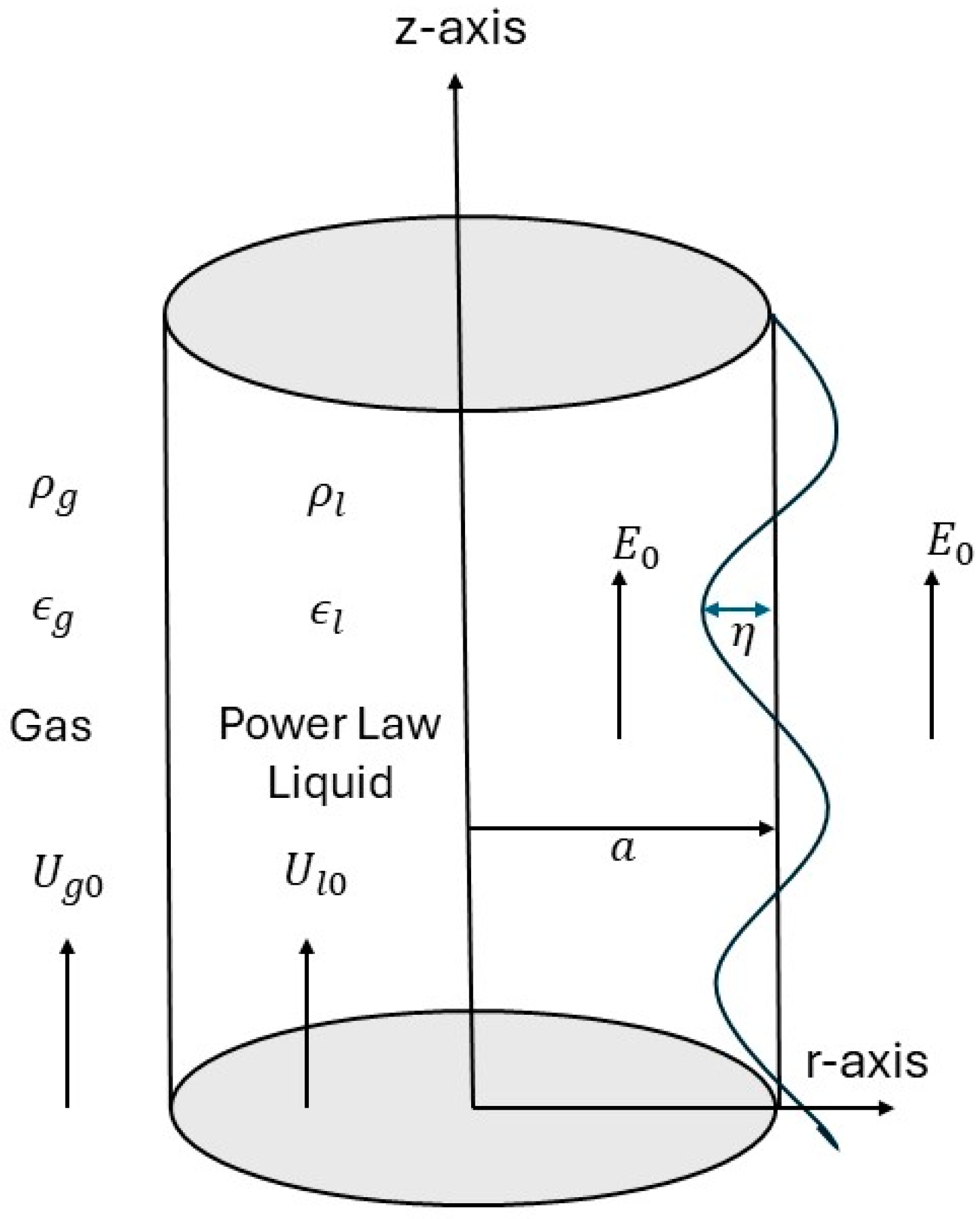
We consider an axisymmetric dielectric P-L liquid jet streaming at an axial velocity in an inviscid dielectric gas medium of density , pressure , and dielectric constant moving with an axial velocity . The jet has consistency coefficient , P-L exponent , radius , density , pressure , dielectric constant , and surface tension . It is assumed that the media in both phases have medium permeability and porosity . A homogeneously applied EF acting in the same direction of flows as and affects the whole system. A sketch of the base flow and the system of coordinates are shown in Figure 1. The two-dimensional cylindrical coordinate system has its origin on the jet axis, the -axis parallel to the direction of the jet flow, and the r-axis is normal to it. It is assumed that the fluids are incompressible, since the velocities and are negligible concerning the speed of sound. The present study investigates the behavior of a non-Newtonian (power-law) fluid jet issuing through a permeable medium into a gaseous streaming environment, where both the porous structure and the surrounding flow field significantly influence the dynamics. The power-law nature of the fluid introduces shear-dependent viscosity, which leads to nonlinear velocity profiles and complex flow behavior, especially within confined or porous domains.
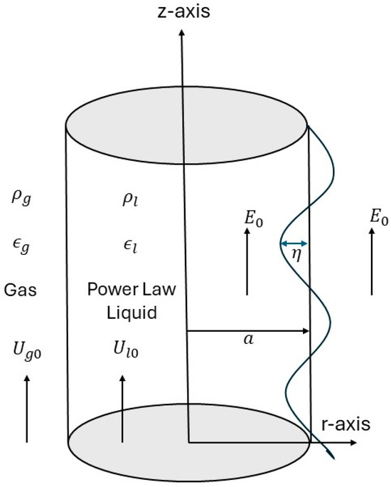
Figure 1.
Schematization of the theoretical physical situation.
The governing equations for momentum and mass preservation in both gas and liquid states are provided by [25].
where is the time and is the extra stress tensor of the fluid jet defined as
Here, stands for the flow behavior index, is the consistency factor, is the strain tensor, is the velocity gradient, and is its transpose. It should be noted that, depending on the amount of , P-L fluids can be ordered as s-thin when , Newtonian when , and s-thick when .
Also, Maxwellian equations, when the quasi-static approximation is considered (i.e., when , with being electric potential), can be written in the two regions in the formula [33].
where the indices ) denote the quantities in both liquid and gas media, respectively. We must make certain approximations to solve the liquid’s equations of motion. When the disturbance is minimal and the liquid jet is seen as vertical, the azimuthal and shear stresses are disregarded, making Equations (1) and (2) obsolete.
where
For the gas phase, Equations (3) and (4) yield the following:
3. Perturbation Equations
The basic states that satisfy equations of motion in both media are
and
The interface between liquid and gas will move away from the position when the jet is disturbed, hence we can write
where is the unit vector in the -direction and is the elevation of the interface from the balance position. In this case, Equations (6) and (7), with the help of Equation (17), yield
To acquire the answers, one must linearize the governing Equations (8)–(10) while maintaining the P-L’s nonlinear characteristics. The velocity component , which is connected to the fluid’s characteristics, is expressed by adding a new coefficient [16]. Consequently, Equation (11) yields
The right-hand side of Equation (19) may be expanded and neglect the higher-order terms, as follows:
The disturbed variables given by Equation (17) can be replaced by the system of Equations (8)–(10), (12)–(14), and (18) above, with the help of Equation (20). That way, the nonlinear components may be disregarded.
4. Normal Modes Analysis and Solutions
As stated in the normal modes form, the temporal linear instability analysis in the current study suggests that the liquid jet is impacted by a little disturbance. We suppose that all perturbation quantities are represented by [49], as is common.
where is the wave number (WN) of the disturbance and . The amplitude of the initial disturbance is lower than the jet radius . It should be noted that, in the analysis of temporally increasing disturbances, is real, and the unstable or stable disturbances are given by , respectively [50], while, when , the system is neutrally stable.
One may derive the linearized equations for the disturbed flow in the two phases by disregarding the nonlinear components and inserting Equation (28) into Equations (21)–(27).
To solve Equations (30) and (31), we express velocities and in following the form:
Therefore, continuity Equation (29), yields the following modified Bessel differential equation:
where
The solution of Equation (38), using Equation (28), is obtained as
Substituting Equations (28) and (40) in Equations (36) and (37), we obtain the following solutions:
Similarly, for the gas medium, we have obtained the following solutions:
In Equations (40)–(45), and are constants to be determined using the BCs, while or and or are the -order modified Bessel functions of 1st and 2nd kinds, respectively [51].
Next, Equation (35) reduces to the modified Bessel differential equation as follows:
The potential functions in the two media may be expressed as follows, after solving Equation (46):
where and are integration constants to be determined via the corresponding BCs.
5. BCs and Dispersion Relationship
The appropriate BCs at the interface () must be satisfied by the solutions of the equations. Therefore, the requirements listed below ought to be met at the interface [16,31], as follows:
Substituting from Equations (28), (41), (42), and (44) into the BCs (49)–(52) and solving the obtaining equations with the help of relations [51] and , we obtain the following:
Therefore, Equations (40)–(42) for the liquid phase reduce to
Similarly, Equations (43)–(45) for the gas phase reduce to
Solutions (47) and (48) of the electric potential functions reduce to
Finally, substituting from Equations (28), (57), (60), and (63) into the condition (53) at yields a dispersion relation in the following form:
Note that for theoretical verification, when , (non-porous media) and , Equation (64) reduces to the following form:
This mathematical form (65) recovered the results achieved before by Chang et al. [16], in which here is replaced by and here is replaced by , ignoring the previous factors. Also, in the absence of a porous medium and an electric field, the dispersion relation (65) can be obtained from the dispersion relation obtained by Guo et al. [52,53] by ignoring the gas cross flow (when ) and the disturbance mode (), respectively. This was also obtained by Wang et al. [54] by ignoring the gas rotational strength and the disturbance mode m for the axisymmetric case . Consequently, given the impacts of the parameters included in this study, flow instability may be reasonably predicted by our suggested model.
Equation (64) can be written in the following dimensionless form:
such that
where , , , and , , , , , , , , , , , .
6. Results and Stability Discussion
The dispersion relation (66) can be solved numerically using Mathematica software (version 12.1) to obtain positive real values of the disturbance growth level . It should be noted that the flow is stable or unstable when , and neutrally stable when . Following the novel procedure of El-Sayed and Alanzi [48], by assuming , and suppose that (for example) as an initial value for the root, we obtained by iteration the solution as the ordered pairs . Figure 2, Figure 3, Figure 4, Figure 5, Figure 6, Figure 7, Figure 8, Figure 9, Figure 10, Figure 11, Figure 12 and Figure 13 listed below give versus to show the influences of other physical parameters on the system’s instability.
It will be demonstrated that every curve in the figures increases monotonically up to a point at which the extreme growth rate is attained, after which the curves start to shrink and eventually cross the WN -axis (cut-off WN) [55]. Furthermore, the WN at which the growth level is greatest is known as the dominant WN. The disintegration of P-L fluid jets in s-thin and s-thick fluids can be categorized into two types of instability modes: RM and TM. In these cases, the jets’ breakup scale is either larger or significantly smaller than the nozzles’ feature scale. The breakup of fluid jets is related to the dominant WN and maximal growth level in these two modes.
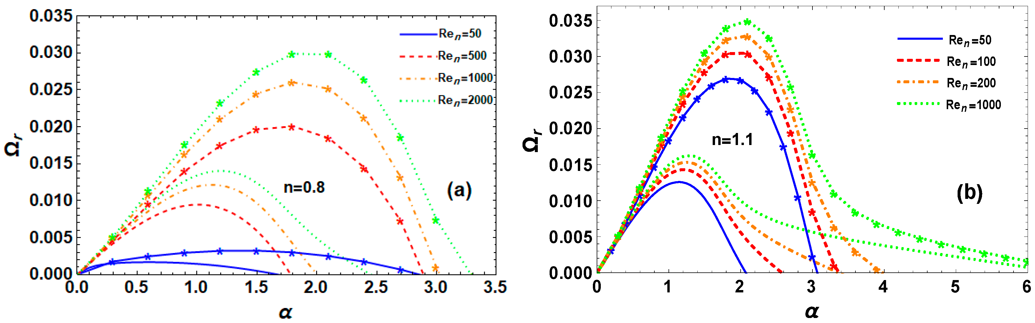
6.1. Impact of
Figure 2a,b shows the impacts of on the instability of an electrified P-L fluid jet in a porous medium under certain conditions for the s-thin and s-thick fluids, respectively. It is noted from Figure 2a,b that the maximal growth level, as well as cut-off WNs, increase as increases in RM (normal curves) and TM (curves with star) for both fluids. In addition, for the s-thin fluid in Figure 2a, the growth rate is near zero, which represents the system’s instability. For the s-thick fluid, when is larger than some values in Figure 2b, the maximal growth rate and dominant WN slightly increase . In this instance, however, the cut-off WNs for both instability modes exceed their values in the s-thin fluid. The findings also show that the P-L liquid jet’s viscous forces always keep it from shattering because of the destabilizing influence on the system under consideration.
Figure 2.
Impact of on for RM (normal curves, ) and TM (curves with star, ) at , , , , , , , , and for (a) s-thin fluid and (b) s-thick fluid.
Figure 2.
Impact of on for RM (normal curves, ) and TM (curves with star, ) at , , , , , , , , and for (a) s-thin fluid and (b) s-thick fluid.
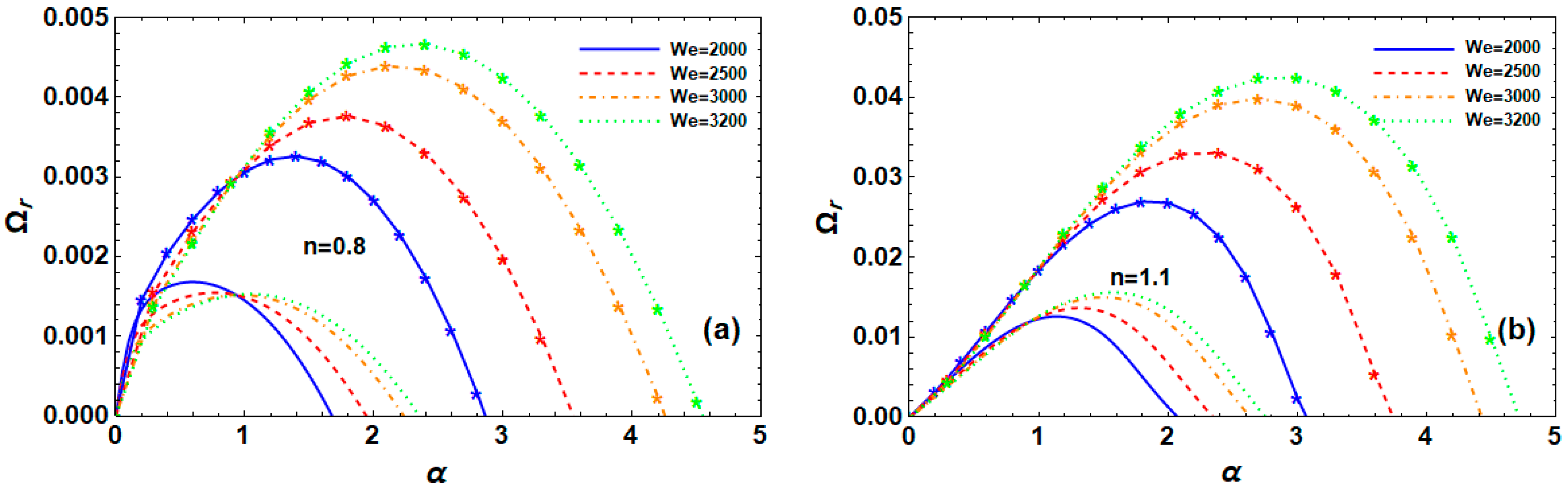
6.2. Effect of We
Instability curves of P-L fluid jets with varying values are displayed in Figure 3a,b for the s-thick and s-thin fluids in TM and RM instability, respectively. The s-thin fluid in Figure 3a has a fixed WN in RM, which causes the growth levels to decrease before and increase with increasing values in such a way that cut-off WNs increase and the maximum growth levels and dominant WNs in RM decrease. The maximal growth level, dominant, and cut-off WNs for TM are shown in the same figure; however, they rise when the value grows after the fixed WN value. As a result, we show that the system plays a dual function in instability, acting as stabilizing and destabilizing forces for both kinds of instability. The instability in TM holds more quickly than it does in RM. The maximum growth level, dominant, and cut-off WNs, as well as the value for RM and TM instability, all increase for the s-thick fluid in Figure 3b. As a result, in this case has a destabilizing influence, making TM more unstable than RM. Furthermore, in s-thick fluid, as opposed to s-thin fluid, it is more vital.
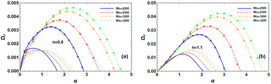
Figure 3.
Impact of on for RRM (normal curves, ) and TM (curves with star, ) at , , , , , , , , and for (a) s-thin fluid and (b) s-thick fluid.
Figure 3.
Impact of on for RRM (normal curves, ) and TM (curves with star, ) at , , , , , , , , and for (a) s-thin fluid and (b) s-thick fluid.
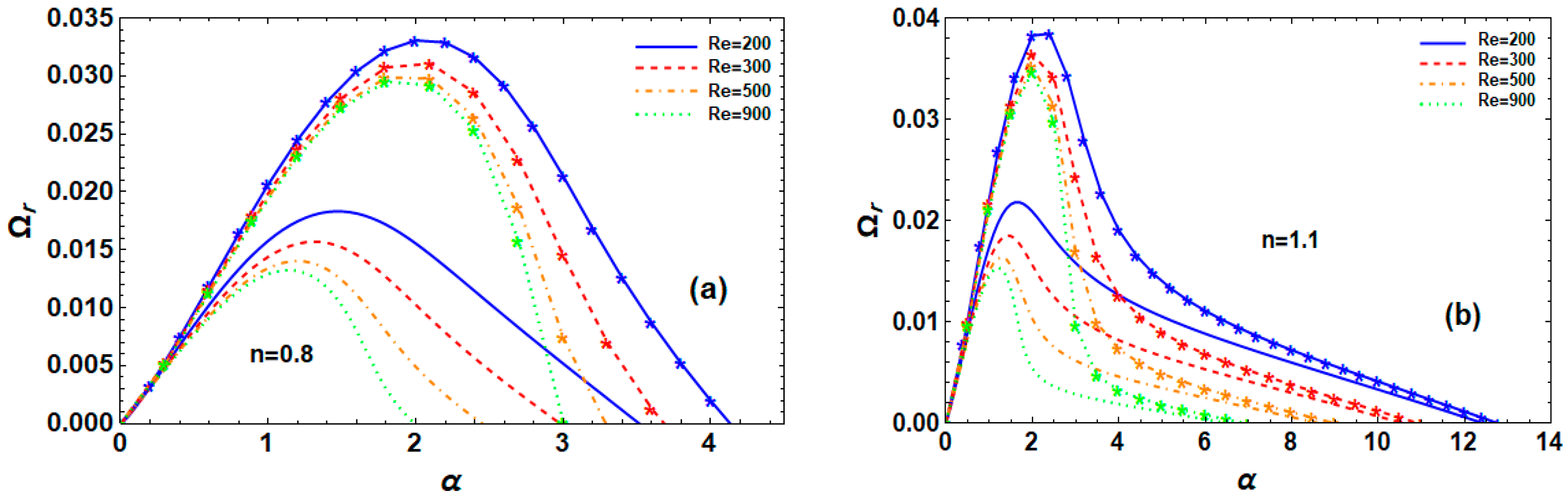
6.3. Effect of
The electrified P-L fluid jets’ instability curves for varying values in the s-thin and s-thick scenarios are illustrated in Figure 4a and Figure 4b, respectively. Except for , which increases from 200 to 900, they show the influences of on the maximal growth level, dominant, and cut-off WNs for RM and TM instability under the previously stated parameters. The maximal growth level, dominant, and cut-off WNs drop in these two modes as increases, as seen for the s-thin fluid in Figure 4a. However, for varying , the maximal growth level is smaller in RM than in TM. Consequently, one may observe that, in TM, the jet breakup is simpler. Keep in mind that the jet’s unstable range is greater in TM than it is in RM. In addition, Figure 4b illustrates that the s-thick fluid is more unstable than the s-thin case depicted in Figure 4a. Additionally, this phenomenon demonstrates that has a stabilizing influence, since cut-off WNs coincide in s-thick for both RM and TM instability.
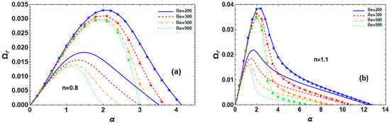
Figure 4.
Impact of on for RM (normal curves, ) and TM (curves with star, ) at , , , , , , , , and for (a) s-thin fluid and (b) s-thick fluid.
Figure 4.
Impact of on for RM (normal curves, ) and TM (curves with star, ) at , , , , , , , , and for (a) s-thin fluid and (b) s-thick fluid.
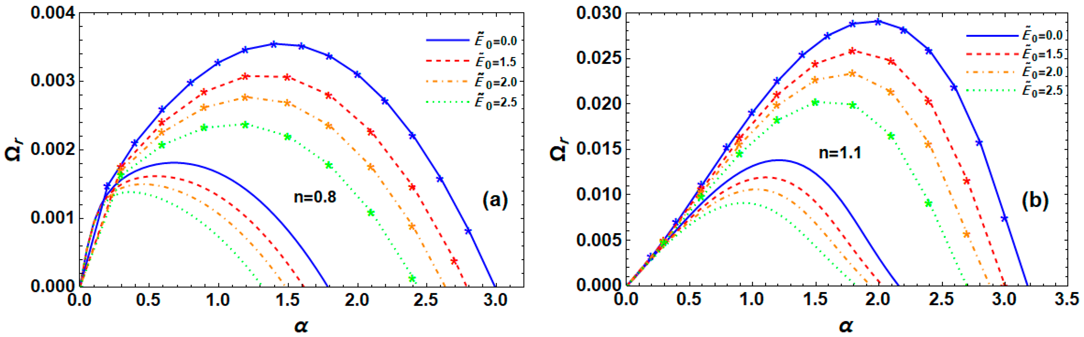
6.4. Effect of Applied Field
The instability curves of electric P-L liquid jets with varying applied fields in s-thin and s-thick fluids are presented in Figure 5a and Figure 5b, respectively. They demonstrate how the maximal growth level, dominant, and cut-off WNs for RM and TM instability at the previously stated circumstances are affected by the presence or absence of the applied field. The maximal growth level, dominant, and cut-off WNs in these two modes decrease with the increasing applied field, as seen for the s-thin fluid in Figure 5a. However, for a given applied field value, the maximal growth level is smaller in RM than in TM. Consequently, we deduce that TM facilitates the breakdown of the P-L liquid jet more easily than RM. Additionally, Figure 5b shows that, in the absence of applied field, the s-thick fluid scenario is more unstable than the analogous s-thin fluid instance shown in Figure 5a. As a result, breaking apart is simpler there than it is in the other two categories of instability. This phenomenon demonstrates that, regardless of whether the fluid is s-thin or s-thick, the applied field often has stabilizing impacts on the P-L liquid system.
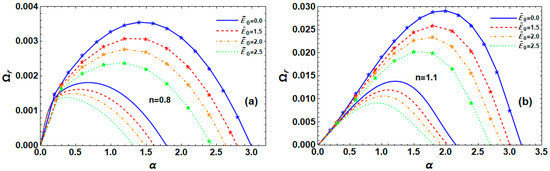
Figure 5.
Impact of on for RM (normal curves, ) and TM (curves with star, ) at , , , , , , , , and for (a) s-thin fluid and (b) s-thick fluid.
Figure 5.
Impact of on for RM (normal curves, ) and TM (curves with star, ) at , , , , , , , , and for (a) s-thin fluid and (b) s-thick fluid.
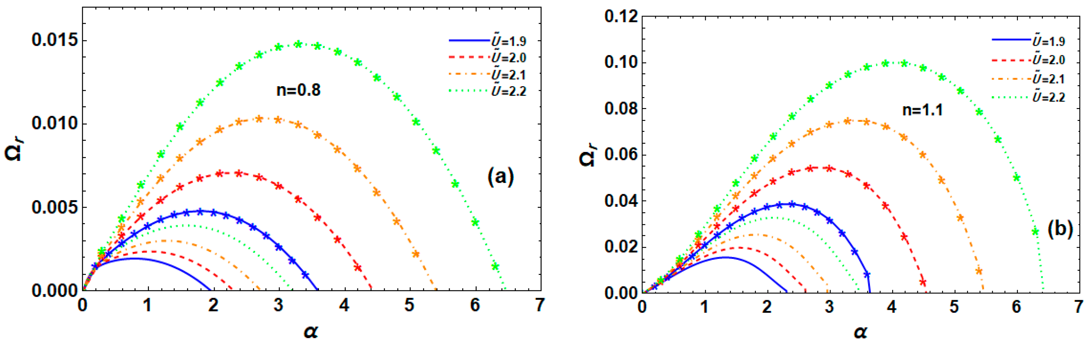
6.5. Effect of P-L Exponent Index
Figure 6a,b illustrates the impacts of the P-L exponent index on the instability of the electrified jets for s-thin (), s-thick (), and Newtonian () fluids for porous and non-porous media, respectively. RM and TM are investigated in each figure when the P-L exponent index differs from one significantly while preserving the clarity of the other physical features. As seen in Figure 6a for the porous medium, the cut-off WNs in RM and TM overlap, whereas the maximal growth level and dominant WNs rise as the P-L exponent index () increases. This indicates that when the P-L index rises in the two instability modes, the P-L liquid jet becomes more unstable. The scenario when () exhibits similar behavior, with the exception that as n values grow, so do the cut-off WNs. Additionally, Figure 6b illustrates that, for non-porous media, the cut-off WNs coincide in both RM and TM for all P-L exponent index values, but the maximal growth levels and dominant WNs rise with increasing P-L exponent index . Furthermore, for a given P-L index n, the liquid jet’s RM has a lower maximum growth level than its TM. When Figure 6a,b are compared, one can declare that the maximum growth level in Figure 6a with a porous medium is much larger than it is in Figure 6b with a non-porous medium. This indicates that the presence of a permeable medium can increase the instability of the P-L fluid flow and make it easier for it to break up in the two modes of instability for both fluids.
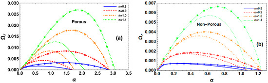
Figure 6.
Impact of P-L exponent index on for RM (normal curves, ) and TM (curves with star, ) at , , , , , , , , , and for (a) porous medium and (b) non-porous medium.
Figure 6.
Impact of P-L exponent index on for RM (normal curves, ) and TM (curves with star, ) at , , , , , , , , , and for (a) porous medium and (b) non-porous medium.
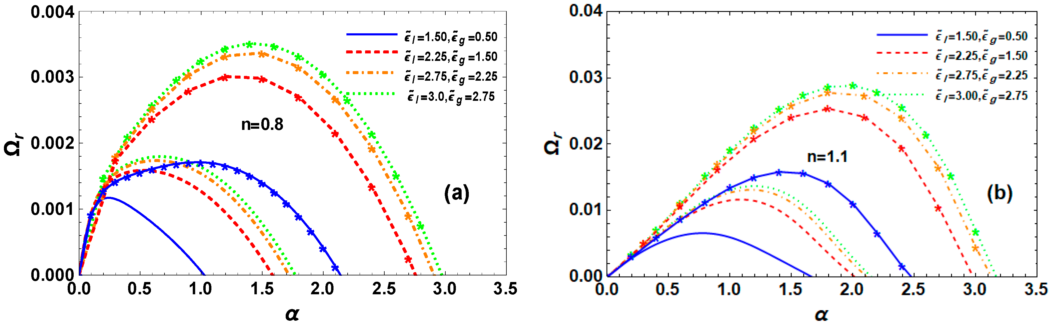
6.6. Effect of Dielectric Constants
The instability curves of electrified P-L fluid jets with varying dielectric constants in s-thin and s-thick fluids are presented in Figure 7a and Figure 7b, respectively. Under the previously stated parameters, they demonstrate how dielectric constants affect the maximum growth level, dominant, and cut-off WNs for RM and TM instability. The s-thin fluid in Figure 7a has a fixed WN in both RM and TM, after which the growth levels increase with increasing values, resulting in an increase in the maximum growth levels, dominant, and cut-off WNs. This occurs before the growth rates decrease for small WN values. Additionally, take note of the fact that, in this instance, the growth rates for RM and TM of instability coincide for tiny WN values. Therefore, we show that the system plays two roles in instability, as follows: stabilizing or destabilizing influence, according to the range of WNs that is small or big for each of the two instability modes. Then, have a destabilizing influence on this system because, in the s-thick fluid shown in Figure 7b, the maximal growth level, dominant, and cut-off WNs all increase due to increasing dielectric constant values for both RM and TM instability. Consequently, since the jet’s unstable range is greater in TM than it is in RM, we conclude that the P-L fluid jet breakup is simpler in TM. Additionally, we may conclude that the s-thick fluid is more unstable than the s-thin fluid in this case. This event demonstrates how the investigated liquid jet system is destabilized by the dielectric constants.
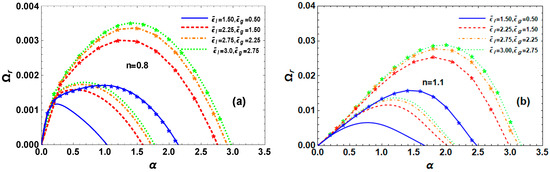
Figure 7.
Impact of dielectric constants , on for RM (normal curves, ) and TM (curves with star, ) at , , , , , , , and for (a) s-thin fluid and (b) s-thick fluid.
Figure 7.
Impact of dielectric constants , on for RM (normal curves, ) and TM (curves with star, ) at , , , , , , , and for (a) s-thin fluid and (b) s-thick fluid.
6.7. Effect of Porosity of Permeable Media
In both RM and TM, Figure 8a,b illustrates how the porosity affects the instability of electrified P-L liquid jets under certain circumstances for s-thin and s-thick fluids, respectively. Figure 8a,b demonstrates that, in RM and TM for s-thin and s-thick fluids, when the porosity rises, the maximal growth level, as well as dominant and cut-off WNs, fall but remain positive; therefore, they reflect stable waves. For both instability modes, their values in the s-thick fluids are larger than the comparable values in the s-thin fluids. Therefore, we conclude that RM instability is lower than that of TM, and that the stabilizing influence of the porosity on the system is achieved. Additionally, it is clear from Figure 8b that, in both RM and TM, the s-thick fluid is more unstable than the s-thin fluid displayed in Figure 8a.
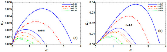
Figure 8.
Impact of porosity on for RM (normal curves, ) and TM (curves with star, ) at , , , , , , , , and for (a) s-thin fluid and (b) s-thick fluid.
Figure 8.
Impact of porosity on for RM (normal curves, ) and TM (curves with star, ) at , , , , , , , , and for (a) s-thin fluid and (b) s-thick fluid.

6.8. Effect of Permeability
For the s-thin and s-thick fluids, respectively, Figure 9a,b illustrate the influences of permeability on the electrified P-L fluid jet’ instability in a porous medium under specific circumstances. For the s-thin fluid, Figure 9a makes it evident that, while the dominant WN remains constant and the cut-off WN marginally lowers with an increase in medium permeability , the maximal growth level drops. The system under examination for TM is likewise shown in Figure 9a to be more unstable than RM. Additionally, Figure 9b for the s-thick fluid makes it evident that, in both RM and TM instability, as the medium permeability rises, the maximal growth level, dominant, and cut-off WNs drop. Thus, we conclude that RM instability is lower than that of TM, and that the medium permeability stabilizes the system under consideration. This phenomenon states that the P-L fluid jet is stable due to the medium permeability and that the stability behavior for both modes remains quicker in a fluid that is s-thin than in a fluid that is s-thick.
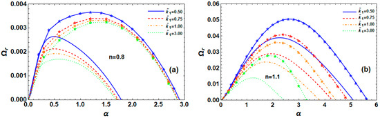
Figure 9.
Impact of medium permeability on for RM (normal curves, ) and TM (curves with star, ) at , , , , , , , , and for (a) s-thin fluid and (b) s-thick fluid.
Figure 9.
Impact of medium permeability on for RM (normal curves, ) and TM (curves with star, ) at , , , , , , , , and for (a) s-thin fluid and (b) s-thick fluid.
6.9. Impact of the Density Ratio
The effects of density ratio on P-L liquid jet’s instability under various situations are illustrated in Figure 10a,b. In both RM and TM instability, the highest growth level and associated WNs increase with the increase in for both the s-thin and the s-thick fluids. However, for the s-thin fluid shown in Figure 10a, the dominant and cut-off WNs are smaller, and the maximum growth level in RM is greater than that observed in TM. Additionally, the maximal growth level, dominant, and cut-off WNs for TM instability in s-thick fluid, shown in Figure 10b, are significantly bigger than their values found in RM instability. These values indicate that RM has somewhat higher maximum growth rates and cut-off WNs. It is found that, in electrified P-L s-thick liquid jets, where TM instability is more relevant than that of RM, the gas-to-liquid density ratio can facilitate the jet’s breakup. Furthermore, whether the fluid is s-thin or s-thick, dominates the growth level of two modes for small and large WNs. Therefore, we have made the decision that our system in operation has been destabilized due to the density ratio .
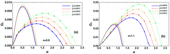
Figure 10.
Impact of on for RM (normal curves, ) and TM (curves with star, ) at , , , , , , , and for (a) s-thin fluid and (b) s-thick fluid.
Figure 10.
Impact of on for RM (normal curves, ) and TM (curves with star, ) at , , , , , , , and for (a) s-thin fluid and (b) s-thick fluid.
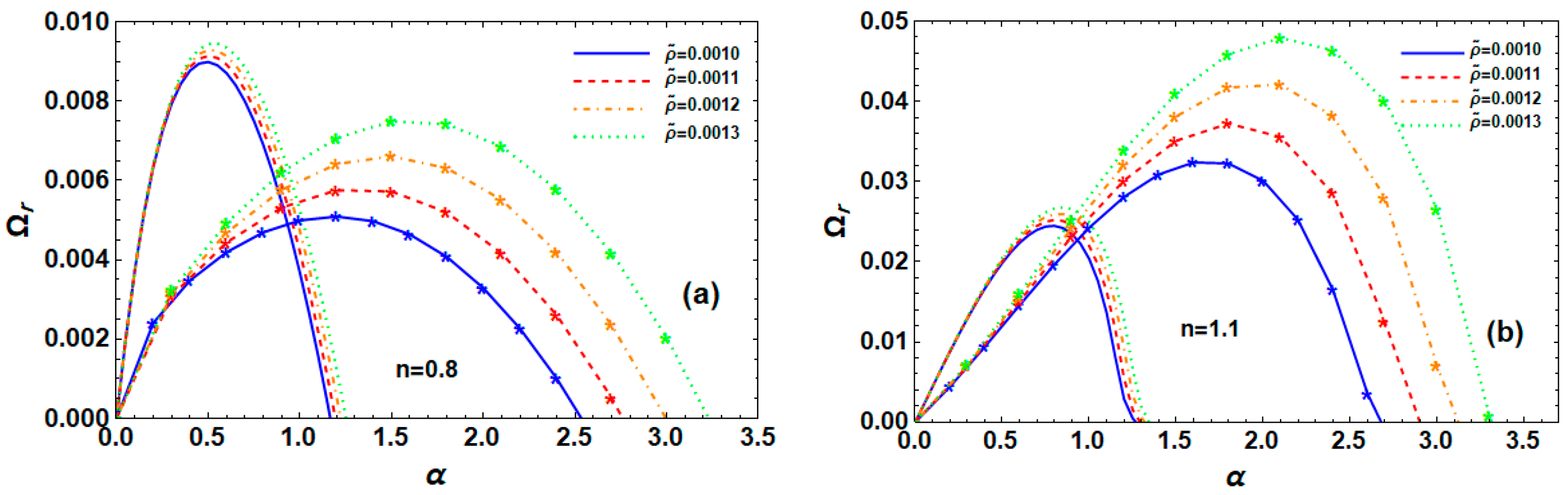
6.10. Effects of Velocity Ratios
For s-thin and s-thick fluids, respectively, Figure 11a,b investigate the impact of velocity ratio on the instability of electrified P-L jets in porous media under specific circumstances. Figure 11a,b demonstrates that, for both s-thin and s-thick fluid instances, the maximum growth level, dominant, and cut-off WNs significantly drop when the velocity ratio rises in RM and TM. Therefore, in this case, the velocity ratio stabilizes the P-L liquid jet system. Additionally, these data demonstrate that, for both fluids, TM’s maximal growth level, dominant WN, and cut-off WNs are larger than those of RM. Moreover, Figure 11b illustrates that the s-thin fluid situation shown in Figure 11a is less unstable than the s-thick fluid case. It is evident that, when gas velocity is absent (), the system becomes more unstable than when for the two fluids and instability modes.
Figure 11.
Impact of on RM (normal curves, ) and TM (curves with star, ) at , , , , , , , , and for (a) s-thin fluid and (b) s-thick fluid.
Figure 11.
Impact of on RM (normal curves, ) and TM (curves with star, ) at , , , , , , , , and for (a) s-thin fluid and (b) s-thick fluid.
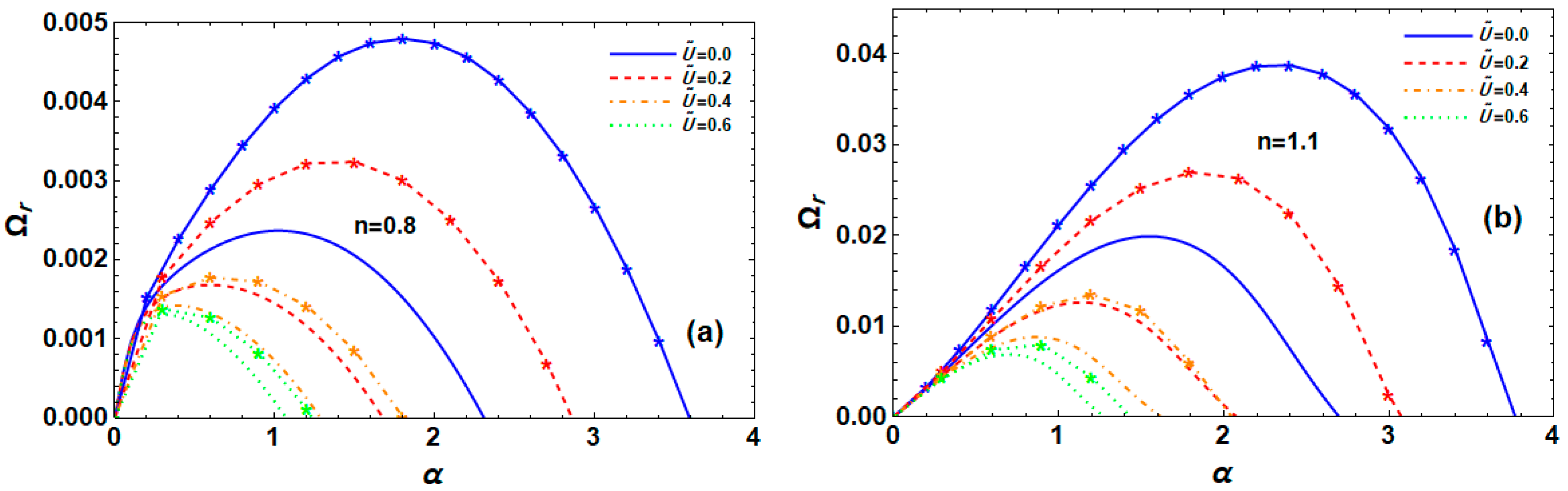
Conversely, Figure 12a,b investigates how the velocity ratio affects the system’s instability when . These results clearly show that, in RM and TM for both fluids, the high growth level, as well as the dominant and cut-off WNs, rise when the velocity ratio . The P-L liquid jet system in porous media is thus destabilized in this scenario by the velocity ratio. Moreover, these data demonstrate that, in both fluids, TM’s maximal growth level, dominant, and cut-off WNs are larger than those of RM. Furthermore, for all values of the velocity ratio, we can observe that the s-thick fluid is more unstable than the s-thin one. Thus, based on Figure 11a,b, and Figure 12a,b, we can deduce that, depending on whether the velocity ratio is more than or less than one, our system of study has two functions in terms of stability.
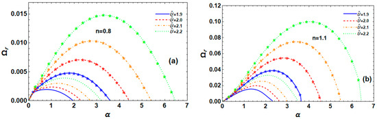
Figure 12.
Impact of on for RM (normal curves, ) and TM (curves with star, ) at , , , , , , , , and for (a) s-thin fluid and (b) s-thick fluid.
Figure 12.
Impact of on for RM (normal curves, ) and TM (curves with star, ) at , , , , , , , , and for (a) s-thin fluid and (b) s-thick fluid.
6.11. Impact of Dynamic Viscosity Ratio
The instability curves of electrified P-L liquid jets with varying viscosity ratios in s-thin and s-thick fluids are presented in Figure 13a and Figure 13b, respectively. When the other parameters stay the same, they demonstrate the impact of equal and varied dynamic viscosities of the dominant, cut-off WNs, and maximal growth level for RM and TM. In these two kinds of instability, when the viscosity ratio grows, the dominant WN remains unchanged, but the maximal growth level and cut-off WN increase, as seen for the s-thin fluid shown in Figure 13a. It has been discovered that the maximal growth levels in TM are larger than those in RM. As a result, in TM, as opposed to RM, the P-L liquid jet’s slightly unstable range is greater. Furthermore, as the maximum growth level, dominant, and cut-off WNs rise with increasing viscosity ratio, Figure 13b illustrates that the s-thick fluid is more unstable than the s-thin one depicted in Figure 13a. This phenomenon demonstrates that the P-L liquid jet system is destabilized by the viscosity ratio and that the instability range is less when the dynamic viscosities are equal than when they are different.
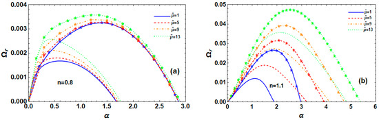
Figure 13.
Impact of on for RM (normal curves, ) and TM (curves with star, ) at , , , , , , , , and for (a) s-thin fluid and (b) s-thick fluid.
Figure 13.
Impact of on for RM (normal curves, ) and TM (curves with star, ) at , , , , , , , , and for (a) s-thin fluid and (b) s-thick fluid.
7. Concluding Remarks
By doing parametric research, a thorough analysis is conducted for stability analysis of an electrified P-L flow jet originating in a flowing dielectric gas through permeable media. An examination of the normal-mode stability of liquid and gas is carried out, taking into account the impact of both the applied field and the permeable medium. The theory yields a dispersion relationship that accounts for the effects of the applied field and properties of the permeable medium. In several instances, the interplay between an EF and a porous material is crucial in ascertaining the flow’s instability properties. It is noted that instability manifests itself in two discrete modes: RM and TM. The data obtained show the following:
- (1)
- For both s-thin and s-thick fluids, the system is more unstable in TM than it is in RM;
- (2)
- Compared to s-thin fluids, the system of s-thick fluids for both modes is more unstable;
- (3)
- Both RM and TM are destabilized by , and the cut-off WNs in the two s-thin fluid modes are less than those in s-thick fluid modes;
- (4)
- In s-thin fluids, has a stabilizing impact for small WNs; however, in s-thick fluids, it has a destabilizing effect for both modes. Afterwards, in both RM and TM, it has a destabilizing influence;
- (5)
- The cut-off WNs are found to coincide for both RM and TM in s-thick fluids at any value, and has a stabilizing influence on our system in both regimes;
- (6)
- For both RM and TM, stabilizes the system of a P-L jet in a porous medium, making RM more stable than TM in both fluids;
- (7)
- In both RM and TM, the P-L exponent index in the existence or absence of a porous medium often has destabilizing effects, and the system’s instability is more unstable in the presence of porous media. When porous media exist in s-thin and Newtonian fluids, the cut-off WNs of the two modes have the same value, otherwise, the cut-off WNs of the two modes coincide;
- (8)
- Depending on the range of WNs, the dielectric constants play two different roles in the stability of s-thin fluids, but they destabilize s-thick fluids;
- (9)
- The dominant WNs remain constant for varying values of medium permeability, while the cut-off WNs in both modes of s-thin fluids are near to each other due to the porosity and permeability . These factors typically have stabilizing effects for both fluids and modes;
- (10)
- The maximal growth level of s-thin fluid is greater in RM than it is in TM, and the opposite is true for s-thick fluid;
- (11)
- The system under investigation is subject to both stabilizing and destabilizing effects depending on the velocity ratios ;
- (12)
- When for RM in s-thin fluid, the system has a stabilizing impact in the WN period . Otherwise, typically has a destabilizing influence on two P-L fluids in RM and TM.
Finally, it should be noted that the current work focuses on single-phase flow. Similar work on EHD multiphase is rarely reported, such as the investigations of Almasi et al. [56] and recently by Wang et al. [57]. Hence, we can extend our work in the near future to a multiphase case, because multiphase EHD flows are of great practical interest, such as in the study of droplet jets and emulsions, while investigating single-phase models provides crucial insights into the fundamental mechanisms of electrohydrodynamics.
Author Contributions
M.F.E.-S.: theorized the work; inscribed the original draft preparation; participated in the methodology; coordinated and revised the manuscript; and validated the results. M.F.E.A.: participated in the methodology; analyzed the equations and solutions; prepared the figures; wrote the discussion; and reviewed and edited the manuscript. D.M.M.: took part in the approach; examined and edited the article; and examined the equations and solutions. All authors have read and agreed to the published version of the manuscript.
Funding
We did not receive any funding for our research work.
Data Availability Statement
All data generated or analyzed during this study are included in this manuscript.
Conflicts of Interest
The authors declare no conflicts of interest.
References
- Lin, S.P.; Kang, D.J. Atomization of a liquid jet. Phys. Fluids 1987, 30, 2000–2006. [Google Scholar] [CrossRef]
- Lin, S.P.; Lian, Z.W. Mechanisms of the breakup of liquid jets. AIAA J. 1990, 28, 120–126. [Google Scholar] [CrossRef]
- Li, X. Mechanism of atomization of a liquid jet. At. Sprays 1995, 5, 89–105. [Google Scholar] [CrossRef]
- Funada, T.; Joseph, D.D.; Yamashita, S. Stability of a liquid jet into incompressible gases and liquids. Int. J. Multiph. Flow 2004, 30, 1279–1310. [Google Scholar] [CrossRef]
- Li, F.; Yin, X.Y.; Yin, X.Z. Linear instability analysis of an electrified coaxial jet. Phys. Fluids 2005, 17, 077104. [Google Scholar] [CrossRef]
- Lin, S.P. Breakup of Liquid Sheets and Jets, 2nd ed.; Cambridge University Press: New York, NY, USA, 2010. [Google Scholar]
- Brenn, G.; Liu, Z.; Durst, F. Linear analysis of the temporal instability of axisymmetric non-Newtonian liquid jets. Int. J. Multiph. Flow 2000, 26, 1621–1644. [Google Scholar] [CrossRef]
- Liu, Z.; Liu, Z. Instability of a viscoelastic liquid jet with axisymmetric and asymmetric disturbances. Int. J. Multiph. Flow 2008, 34, 42–60. [Google Scholar] [CrossRef]
- El-Sayed, M.F.; Moatimid, G.M.; Elsabaa, F.M.F.; Amer, M.F.E. 3-dimensional instability of non-Newtonian viscoelastic liquid jets issued into a streaming viscous (or inviscid) gas. Int. J. Fluid Mech. Res. 2017, 44, 93–113. [Google Scholar] [CrossRef]
- Khodayari, H.; Ommi, F.; Saboohi, Z. Investigation of the primary breakup length and instability of non-Newtonian viscoelastic liquid jets. Int. J. Multiphysics 2018, 12, 327–348. [Google Scholar]
- Andersson, H.L.; Irgens, F. Film flow of power law fluids, Encyclopedia Fluid Mech. Polymer Flow Eng. 1989, 9, 617–648. [Google Scholar]
- Gao, Z.; Ng, K. Temporal analysis of power-law liquid jets. Comput. Fluids 2010, 39, 820–828. [Google Scholar] [CrossRef]
- Yang, L.J.; Du, M.L.; Fu, Q.F.; Zhang, W. Linear stability analysis of a power-law liquid jet. At. Sprays 2012, 22, 123–141. [Google Scholar] [CrossRef]
- Ertl, M.; Weigand, B. Analysis methods for DNS of primary breakup of shear-thinning liquid jets. At. Sprays 2017, 27, 303–317. [Google Scholar] [CrossRef]
- Kitamura, Y.; Takahashi, T. Breakup of jets in power law non-Newtonian liquid systems. Can. J. Chem. Eng. 1982, 60, 732–737. [Google Scholar] [CrossRef]
- Chang, Q.; Zhang, M.Z.; Bai, F.Q.; Wu, J.P.; Xia, Z.Y.; Jiao, K.; Du, Q. Instability analysis of a power law liquid jet. J. Non-Newton. Fluid Mech. 2013, 198, 10–17. [Google Scholar] [CrossRef]
- Deng, H.Y.; Feng, F.; Wu, X.S. Dual-mode linear analysis of temporal instability for power-law liquid sheet. At. Sprays 2016, 26, 319–347. [Google Scholar] [CrossRef]
- Wang, X.T.; Ning, Z.; Lu, M.; Sun, C.H. Temporal analysis of breakup for a power-law liquid jet in a swirling gas. Meccanica 2018, 58, 2067–2078. [Google Scholar] [CrossRef]
- Nsom, B.; Ramifidisoa, L.; Latrache, L.; Ghaemizadeh, F. Linear stability of s-thin fluid down an inclined plane. J. Mol. Liquids 2019, 277, 1036–1046. [Google Scholar] [CrossRef]
- Guo, J.P.; Wang, Y.B.; Bai, F.Q.; Du, Q. Instability breakup model of power-law fuel annular jets in slight multiple airflows. Phys. Fluids 2020, 32, 094109. [Google Scholar] [CrossRef]
- Liu, W.M.; Chen, C.K. Stability analysis of thin power-law fluid film flowing down a moving plane in a vertical direction. Fluids 2022, 7, 167. [Google Scholar] [CrossRef]
- Greenkorn, R.A. Flow Phenomena in Porous Media: Fundamentals and Applications in Petroleum, Water, and Food Production; Marcel Dekker: New York, NY, USA, 1984. [Google Scholar]
- Pop, I.; Ingham, D.B. Convective Heat Transfer: Mathematical and Computational Modeling of Viscous Fluids and Porous Media; Pergamon Press: Oxford, UK, 2001. [Google Scholar]
- Bejan, A. Porous and Complex Flow Structure in Modern Technologies; Springer: Berlin, Germany, 2004. [Google Scholar]
- Straughan, B. Stability and Wave Motion in Porous Media; Applied Mathematical Sciences; Springer: New York, NY, USA, 2008; Volume 165. [Google Scholar]
- Nield, D.A.; Bejan, A. Convection in Porous Media, 4th ed.; Springer Science+ Business Media: New York, NY, USA, 2013. [Google Scholar]
- Sochi, T. Non-Newtonian flow in porous media. Polymer 2010, 51, 5007–5023. [Google Scholar] [CrossRef]
- Sochi, T. Flow of non-Newtonian fluids in porous media. J. Polym. Sci. Part B Polym. Phys. 2010, 48, 2437–2467. [Google Scholar] [CrossRef]
- Amaouche, M.; Djema, A.; Abderrahmane, H.A. Film flow for power-law fluids: Modeling and linear stability. Eur. J. Mech.-B/Fluids 2012, 34, 70–84. [Google Scholar] [CrossRef]
- Longo, S.; Federico, V.D. Stability analysis of gravity currents of a power law liquid in a porous medium. Math. Probl. Eng. 2015, 2015, 286487. [Google Scholar] [CrossRef]
- El-Sayed, M.F.; Moatimid, G.M.; Elsabaa, F.M.F.; Amer, M.F.E. Axisymmetric and asymmetric instabilities of a non-Newtonian liquid jet moving in an inviscid gas through porous media. J. Porous Media 2016, 19, 751–769. [Google Scholar] [CrossRef]
- Airiau, C.; Bottaro, A. Flow of shear-thinning fluids through porous media. Adv. Water Resour. 2020, 143, 103658. [Google Scholar] [CrossRef]
- Melcher, J.R. Continuum Electromechanics; MIT Press: Cambridge, MA, USA, 1981. [Google Scholar]
- David, J.G. Introduction to Electrohydrodynamics; Prentice Hall International, Inc.: Hoboken, NJ, USA, 1999. [Google Scholar]
- Nayyar, N.K.; Murty, G.S. The stability of a dielectric liquid jet in the presence of a longitudinal electric field. Proc. Phys. Soc. 1960, 75, 369–373. [Google Scholar] [CrossRef]
- Schneider, J.M.; Lindblad, N.R.; Hendricks, C.D.; Crowley, J.M. Stability of an electrified liquid jet. J. Appl. Phys. 1967, 38, 2599–2605. [Google Scholar] [CrossRef]
- Turnbull, R.I. On the instability of electrostatistically sprayed liquid jet. IEEE Trans. Ind. Appl. 1992, 28, 1432–1438. [Google Scholar] [CrossRef]
- El-Sayed, M.F.; Syam, M.I. Numerical study for the electrified instability of viscoelastic cylindrical dielectric fluid film surrounded by a conducting gas. Phys. A Stat. Mech. Its Appl. 2007, 377, 381–400. [Google Scholar] [CrossRef]
- Ozgen, S.; Uzol, O. Investigation of the linear stability problem of electrified jets, Inviscid analysis. J. Fluids Eng. 2012, 134, 091201. [Google Scholar] [CrossRef]
- Li, G.; Luo, X.; Si, T.; Xu, R.X. Temporal instability of coflowing liquid-gas jets under an electric field. Phys. Fluids 2014, 26, 054101. [Google Scholar] [CrossRef]
- Rajabi, A.; Morad, M.R.; Rahbari, N. Stability and breakup of liquid jets: Effect of slight gaseous crossflows and electric fields. Chem. Eng. Sci. 2017, 165, 89–95. [Google Scholar] [CrossRef]
- Wang, X.T.; Ning, Z.; Lu, M. Linear instability of a charged non-Newtonian liquid jet under an axial electric field. J. Appl. Phys. 2019, 128, 135301. [Google Scholar] [CrossRef]
- Kaykanat, S.I.; Uguz, A.K. The linear stability between a Newtonian and a power-law fluid under a normal electric field. J. Non-Newton. Fluid Mech. 2020, 277, 104220. [Google Scholar] [CrossRef]
- Del Rio, J.A.; Whitaker, S. Electrohydrodynamics in Porous Media. Transp. Porous Media 2001, 44, 385–405. [Google Scholar] [CrossRef]
- Metwaly, T.M.N.; Hafez, N.M. Electroviscoelastic stability analysis of cylindrical structures in Walters B conducting fluids streaming through porous medium. Fluids 2022, 7, 224. [Google Scholar] [CrossRef]
- Bendel, P.; Bernardo, M.; Dunsmuir, J.H.; Thomann, H. Electric field driven flow in natural porous media. Magn. Reson. Imaging 2003, 21, 321–327. [Google Scholar] [CrossRef]
- El-Sayed, M.F.; Moussa, M.H.M.; Hassan, A.A.A.; Hafez, N.M. Electrohydrodynamic instability of liquid sheet saturating porous media with interfacial surface charges. At. Sprays 2013, 23, 165–191. [Google Scholar] [CrossRef]
- El-Sayed, M.F.; Alanzi, A.M. Electrohydrodynamic liquid sheet instability of moving viscoelastic couple-stress dielectric fluid surrounded by an inviscid gas through porous medium. Fluids 2022, 7, 247. [Google Scholar] [CrossRef]
- Drazin, P.G.; Reid, W.H. Hydrodynamic Stability; Cambridge University Press: New York, NY, USA, 1981. [Google Scholar]
- Charru, F. Hydrodynamic Instabilities; Cambridge University Press: New York, NY, USA, 2011. [Google Scholar]
- Watson, J.N. A Treatise on the Theory of Bessel Functions; Cambridge University Press: Cambridge, UK, 1995. [Google Scholar]
- Guo, J.P.; Bai, F.Q.; Chang, Q.; Du, Q. Investigation on asymmetric instability of cylindrical power-law liquid jets. Energies 2019, 12, 2785. [Google Scholar] [CrossRef]
- Guo, J.P.; Wang, Y.B.; Bai, F.Q.; Du, Q. Unstable breakup of a power-law liquid fuel jet in the presence of a gas crossflow. Fuel 2020, 263, 116606. [Google Scholar] [CrossRef]
- Wang, X.T.; Ning, Z.; Lu, M.; Li, Y.X. Linear stability of a non-Newtonian liquid jet in a coaxial swirling air. Aerosp. Sci. Technol. 2019, 91, 150–158. [Google Scholar] [CrossRef]
- Yang, L.J.; Du, M.I.; Fu, Q.F. Stability of an annular power-law liquid sheet. Proc. Inst. Mech. Eng. Part C 2015, 229, 2750–2759. [Google Scholar] [CrossRef]
- Almasi, F.; Hopp-Hirschler, M.; Hadjadj, A.; Nieken, U.; Shadloo, M.S. Coupled electrohydrodynamic and thermocapillary instability of multi-phase flows using an incompressible smoothed particle hydrodynamics method. Energies 2022, 15, 2575. [Google Scholar] [CrossRef]
- Wang, D.; Chagot, L.; Wang, J.; Angeli, P. Effect of electric field on droplet formation in a co-flow microchannel. Phys. Fluids 2025, 37, 023331. [Google Scholar] [CrossRef]
Disclaimer/Publisher’s Note: The statements, opinions and data contained in all publications are solely those of the individual author(s) and contributor(s) and not of MDPI and/or the editor(s). MDPI and/or the editor(s) disclaim responsibility for any injury to people or property resulting from any ideas, methods, instructions or products referred to in the content. |
© 2025 by the authors. Licensee MDPI, Basel, Switzerland. This article is an open access article distributed under the terms and conditions of the Creative Commons Attribution (CC BY) license (https://creativecommons.org/licenses/by/4.0/).