Choked Flow in Calibrated Orifices for Hydraulic Fluid Power Applications

Abstract

The flow rate through hydraulic resistance increases with the pressure drop across it, but this correlation is no longer valid under cavitation conditions. This study investigates choked flow in calibrated screw-in orifices, widely used for control and damping in fluid power components. An experimental campaign was conducted on orifices with diameters ranging from 1 to 0.4 mm at various upstream pressures using hydraulic oil. A computational fluid dynamics (CFD) model was developed and validated against experiments, then used to analyze the effects of geometric parameters such as edge chamfers, hex wrench sockets, and length-to-diameter ratio. From CFD results, an analytical correlation between flow rate and pressure drop was derived, incorporating flow saturation effects. The study revealed that under saturation conditions, flow rate is largely unaffected by geometry, except for the ideal case of a perfectly sharp-edged orifice, which is rarely encountered. Even minimal chamfers of a few hundredths of a millimeter make the restrictor non-ideal. The derived correlation can be integrated into lumped parameter models of fluid power components to account for choked flow.

1. Introduction

Small, calibrated orifices, with diameters of the order of 1 mm or less, are widely used in fluid power applications for control and damping purposes. In hydraulic piloted pressure control valves, they are used to uncouple the pressures on the two sides of the main poppet or spool, allowing for valve regulation. Moreover, they are used for generating a pressure drop in transient conditions with the aim of generating a damping force on the movable elements of the valve. Small orifices are also employed in hydraulic displacement controls of positive displacement pumps. The volumetric flow rate Q vs. pressure drop (p₁ − p₂) through a restrictor with cross section A is calculated by Equation (1), which is undoubtedly the most used and cited formula in the fluid power field:

$$Q=C_d A \sqrt{{\displaystyle \frac{2 (p_1-p_2)}{\rho }}}$$

(1)

where ρ is the fluid density and C_d the discharge coefficient. The discharge coefficient, when the flow is not fully turbulent, is a function of the Reynolds number and of the specific geometry of the restrictor. Several papers can be found in the open literature concerning the determination of the discharge coefficient in circular section orifices, although most studies consider water as working fluid. For ideal sharp edge restrictors with negligible length and a diameter much smaller than the diameter of the pipe, the value of the discharge coefficient in a turbulent regime is 0.611 [1]. However, such a value is highly influenced by small geometrical modifications.

Studies on the discharge coefficient for orifices under non-cavitating conditions have examined the influence of various geometric and fluid parameters. Key geometric factors include orifice shape, the number of holes in the orifice plate, the length-to-diameter ratio, the orifice-to-pipe ratio, the type of orifice edge, and the orifice angle. Additionally, fluid parameters such as fluid type, viscosity, and temperature are important considerations when determining the discharge coefficient. Together, these factors significantly affect flow characteristics across orifices [2,3,4]. In [5], the discharge coefficient is experimentally measured for orifices with diameters ranging from 12 to 20 mm and thickness of 2.5 mm for Reynolds numbers up to 400. The reference [6] describes a simulation and experimental activity aimed at determining the discharge coefficient in sharp-edge hydraulic orifices with a length-to-diameter (L/D) ratio of 0.3 crossed by two-phase flow (mineral oil and air) up to a Reynolds number of about 600. In [7], a correlation for the discharge coefficient of square-edged concentric orifices in the laminar flow regime is presented, investigating the effects of varying the orifice-to-pipe diameter ratio (ranging from 0.2 to 0.8) and the orifice thickness ratio (spanning from 1/16 to 1) for Reynolds numbers up to 250. Reference [8] presents an experimental investigation of the discharge coefficient for high-viscosity fluids. Specifically, the L/D and the orifice-to-pipe diameter ratio are varied to study the influence of geometry on the discharge coefficient. The study shows that an increase in L/D leads to a higher C_d, but beyond a certain point, excessive L/D causes additional frictional pressure loss, which ultimately reduces the discharge coefficient. In [9], the discharge through micro-orifices with single-phase water flow was experimentally investigated. A multi-micro-orifice piece, consisting of six orifices with a diameter of 200 μm and a length-to-diameter ratio ranging from 4.25 to 27.0, was tested. The Reynolds number was varied between 5 and 4500, transitioning from creeping flow to laminar to turbulent transitional flow. The study demonstrated that L/D is a key factor in controlling the pressure drop under creeping flow conditions, while its influence diminishes at higher Reynolds numbers as the experimental profiles for different L/D values tend to converge. In [10], the impact of orifice angle on the internal flow and discharge characteristics of oil jet nozzles was investigated. The analysis covered orifice angles from 0-degree to 90-degree, with injection pressure differences ranging from 0.1 MPa to 0.5 MPa. The findings revealed that the mass flow rate and discharge coefficient initially decreased and then increased as the orifice angle increased, with a minimum value observed at an orifice angle of 30-degree. In [11], the flow of non-Newtonian fluids through sharp orifices is modeled. Experimental data from fluids with three different viscosities are used to develop a dimensionless relationship among the Euler number, Reynolds number, diameter ratio, and Weissenberg number. The resulting model is applicable for Reynolds numbers ranging from 4 × 10⁻⁵ to 2000 and diameter ratios between 0.04 and 0.16. Another paper [12] presents a study on the fluid mechanics of hydraulic orifices under high (up to 80 °C) and low (down to −10 °C) temperature conditions. A compact experimental module is used to examine the flow characteristics of a sharp-edge hydraulic orifice with L/D = 0.36, using anti-wear hydraulic oil HM46. The study shows that when the temperature drops below room temperature, the discharge coefficient decreases linearly.

The discharge coefficient is also significantly reduced in conditions of cavitation. More specifically, the flow rate through the orifice saturates (choked flow) when the pressure drop across it has reached a critical value. To define the condition of inception cavitation, different cavitation indexes have been defined, involving the inlet and outlet pressures, the vapor pressure and the mean fluid velocity in the orifice. Several studies have been conducted to define the steady-state characteristics of orifices with different geometries. In [13], both acoustic and hydrodynamic cavitation are discussed, along with various models of nozzle discharge coefficients. The physical cause of choked flows is presented, as well as advancements in the characterization of different cavitation regimes in nozzles.

Most of the simulation models have been developed with high-end environments; however, CAD-embedded software, such as Simcenter FloEFD^®, are able to simulate the saturation of the flow rate in a fixed orifice [14]. Furthermore, other simulation tools have been employed in cavitation evaluation. Another paper [15] presents a study, based only on 2D CFD simulations with ANSYS Fluent^®, where the effect of L/D and the inlet fillet radius on cavitation in circular orifices is studied. The most advanced cavitation model (Singhal et al.) was used for simulations. They found that even a small fillet radius at the orifice inlet has a significant effect on the discharge coefficient. In [16], the cavitating flow in a rectangular micro-orifice was studied through CFD simulations with the Zwart–Gerber–Belamri (ZGB) cavitation model. The length-to-width ratio was analyzed. An experimental activity was carried out in [17] on circular micro-orifices with diameters of 150 μm and 300 μm and thickness ranging from 1.04 to 1.93 mm using water as the working fluid in conditions of choked flow. The validation of a CFD model in ANSYS Fluent in a single geometry configuration of a circular orifice is reported in [18]. Another experimental and simulation activity was carried out in [19] regarding the influence of the diameter of circular hole diaphragms in a pipe with a contraction ratio ranging from 0.3 to 0.6. In [20], the cavitation phenomenon in the combustion process of diesel engines is studied. An optimal set of numerical models is identified in ANSYS Fluent, with the k-ω SST (Shear Stress Transport) turbulence model, the ZGB cavitation model, and the VOF (Volume of Fluid) multiphase model providing the best match to experimental results from previous work [21].

As shown, the concept of flow rate saturation due to cavitation is well-established in certain branches of hydraulics, such as water distribution networks, but is often overlooked in the design of conventional mineral-oil-based systems used in both industrial and mobile fluid power applications. In reference [22], among other things, the authors measured the flow rate in orifices with diameters ranging from 1 to 5 mm with L/D ranging from 1 to 3, with and without a 45-degree chamfer under cavitating and non-cavitating flow conditions. In [23], the influence of the type of oil on the cavitation in orifices was studied, and no significant differences in cavitation properties were found. In reference [24], some of the authors of this paper implemented in ANSYS CFX^® a model for gaseous and vapor cavitation. The model was validated on a restriction located in the suction pipe of a pump used in fluid power applications. In [25], a model for predicting gaseous cavitation in hydraulic orifices is presented. Measured mass flow rates from an experimental setup using ISO VG 46 mineral oil are used to calibrate a CFD model developed in ANSYS Fluent. The fluid field simulated by this model is then used to calculate the parameters required for a lumped parameter cavitation model.

Several studies have addressed the challenges in modeling the discharge coefficient for orifices and hydraulic valves under various flow conditions. In [26], a methodology for the parametric modeling of flow rate in different types of hydraulic valves is developed. After identifying the critical restrictions of the valve, the necessary parameters for the parametric function used to model the discharge coefficient are derived by using numerical CFD simulations. In reference [27], a closed-form model for the discharge coefficient as a function of Reynolds number, along with the laminar and turbulent discharge coefficients, is presented. Additionally, a method is introduced to eliminate the need for time-consuming iterative solutions during dynamic simulations.

However, although numerous studies have been conducted on this topic, there is a lack of precise data regarding commercial screw-in orifices for hydraulic fluid power applications, particularly in terms of the discharge coefficient and the maximum flow rate at a given upstream pressure. Specifically, the quantification of the effects of the 60-degree chamfers on the leading and trailing edges, as well as the hex socket recess, has not yet been addressed in the literature. Moreover, the fact that the orifice exhibits asymmetric behavior is often overlooked. Finally, an analytical model for flow rate calculation that incorporates flow saturation independently of operating conditions and L/D has not yet been developed for this specific type of component.

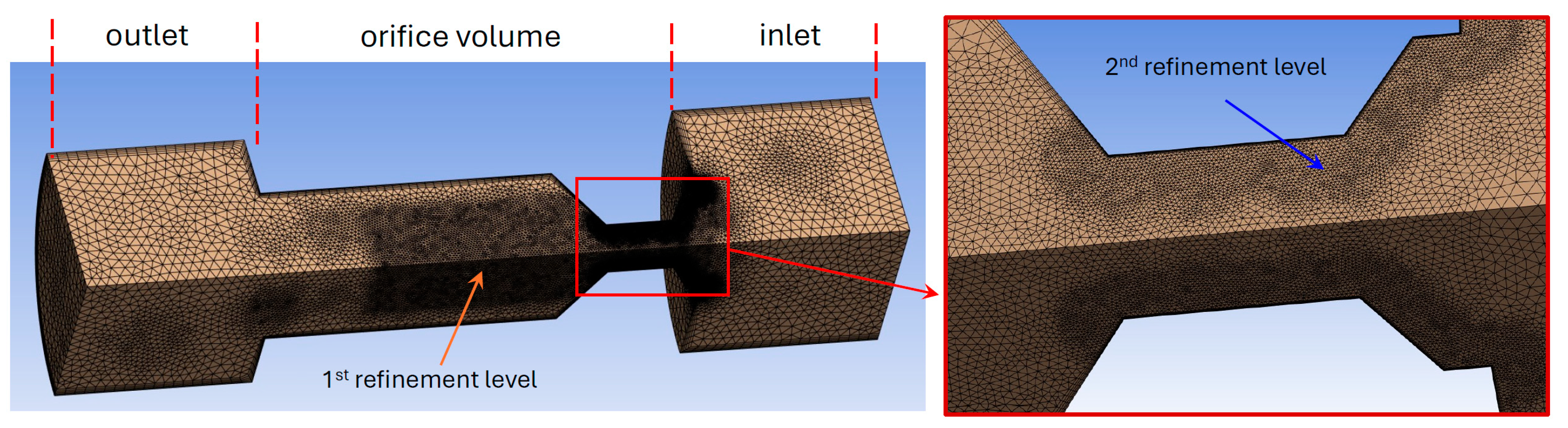
This study aims to fill these gaps by employing a CFD model developed in ANSYS Fluent and experimentally validated on various geometries. The structure of the paper is as follows: Section 2 describes the test bench, while Section 3 presents the characteristics of the model and its validation. Section 4 applies the model to study the influence of certain geometric parameters. Finally, in Section 5, an analytical model is proposed based on the CFD results.

2. Experimental Tests

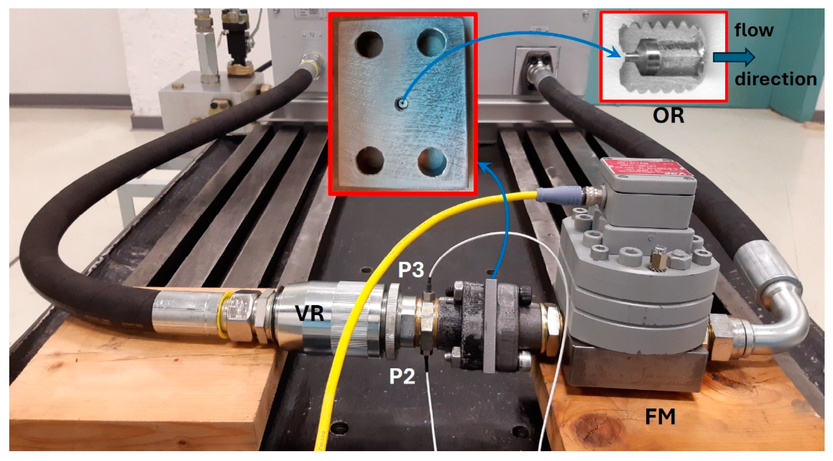
The experimental tests were conducted at the Fluid Power Research Laboratory of the Politecnico di Torino. The hydraulic scheme of the test rig is shown in Figure 1. The flow rate was generated by the main hydraulic power unit of the laboratory, where an axial piston pump equipped with an absolute pressure limiter with setting p* controlled remotely allows the test rig to be fed at constant pressure. A photo of the test rig with a zoomed view of the mounting of one of the orifices under study is reported in Figure 2. The inlet pressure is measured by a pressure transducer (P1) Keller PAA-21Y with range 0 ÷ 400 bar and overall accuracy (including linearity, hysteresis, repeatability, and temperature coefficients) ±1% FS. The flow rate was measured by a gear flow meter (FM), VSE 1 GPO12V, with an accuracy of 0.3% of the measured value and a range of 0.05 ÷ 80 L/min. Under the operating conditions of flow rate and viscosity considered in this study, the pressure drop introduced by the meter in the worst case is approximately 0.1 bar, which is absolutely negligible.

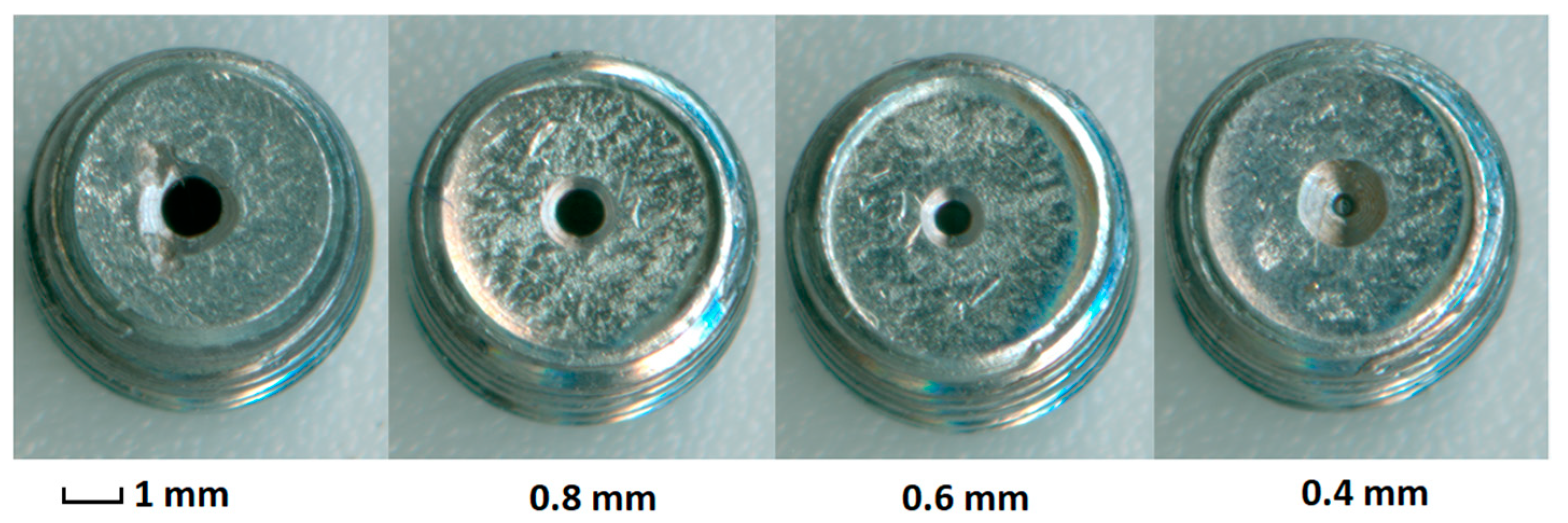
Commercially calibrated orifices (ORs), with diameters of 0.4, 0.6, 0.8, and 1 mm shown in Figure 3, were screwed on a steel plate clamped between two flanges provided with O-rings. The orifices used have a metric M6 thread with a 3 mm hex socket. The seal between the orifice and the plate was also ensured by a PTFE thread seal tape. For maximum reliability, the outlet pressure measurement was performed redundantly as the average of the readings from two miniature transducers screwed onto the hydraulic fitting (P2 and P3): GS XPM5 with a range of 0 ÷ 200 bar and linearity ±0.25% FS, and Entran EPX with a range of 0 ÷ 350 bar. The load at the outlet of the orifice was generated by a manual restrictor (VR). The oil was maintained at 40 ± 1 °C by the fluid conditioning group of the hydraulic power unit, which consisted of a water–oil heat exchanger and a proportional valve for modulating the water flow rate. The entire hydraulic line of the test rig consisted of 1″ pipes, so that the only pressure drops were due to the local restrictions OR and VR, with the maximum flow rate being always lower than 10 L/min. The distance of the variable restrictor from the orifice OR is about 100 mm, while the transducers are located at 50 mm, therefore at a distance 50 times greater than the diameter of the largest tested orifice, in a region where the pressure field has definitely become homogeneous.

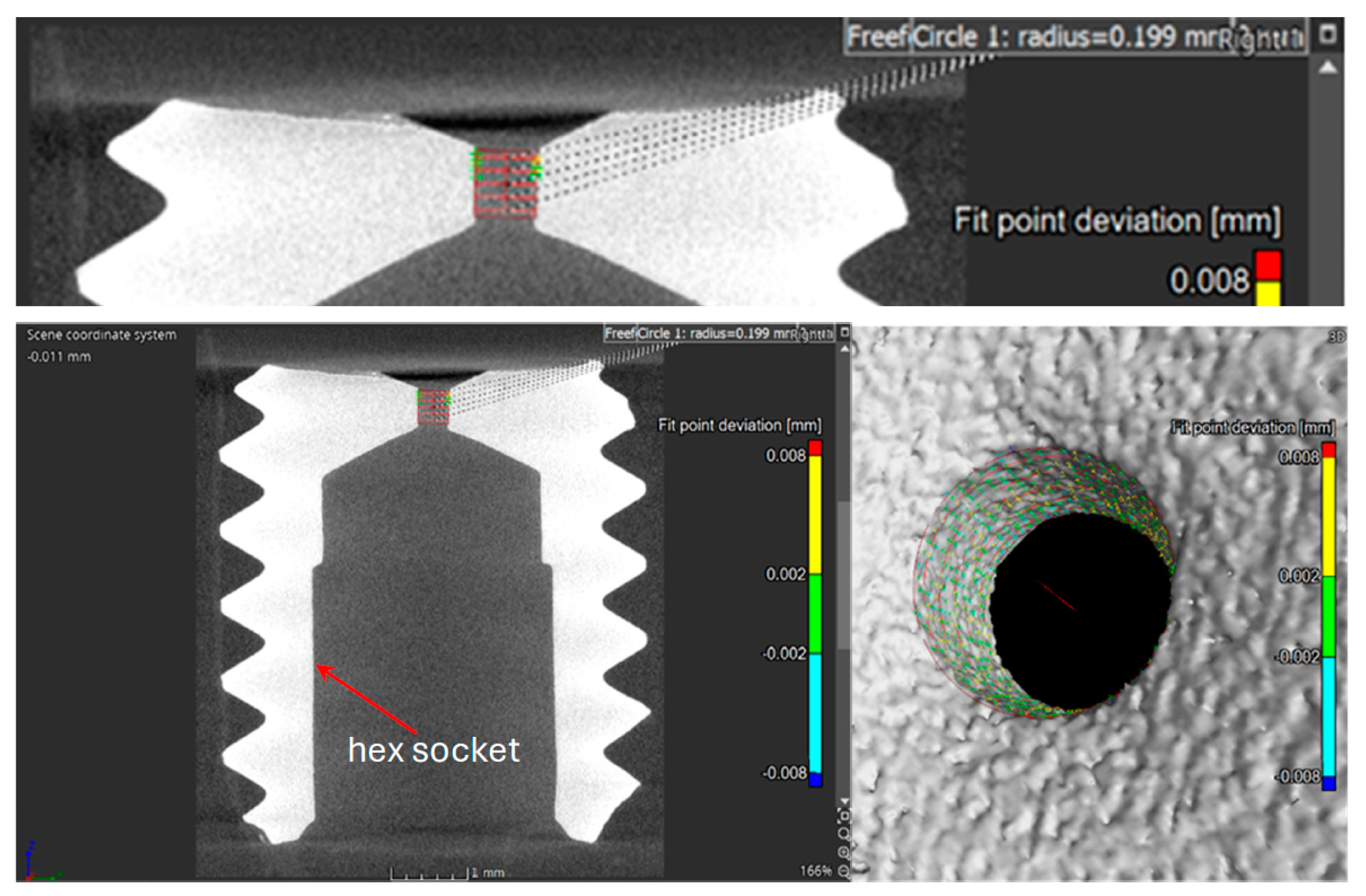
The visual analysis of the orifices highlighted some geometric differences between the various sizes. For example, the chamfer on the orifice with a diameter of 0.4 mm is larger compared to the others. To ensure accurate simulation of the correct geometry, the most critical parameter, i.e., the hole diameter, was measured using X-ray tomography. Figure 4 shows the scan of the 0.4 mm restrictor. The diameter of the larger sizes (1 mm and 0.8 mm) was measured to be a couple of hundredths of a millimeter smaller than the nominal value, and the corrected value was used in the simulations. All the orifices have a length-to-diameter (L/D) ratio of 1. The simulations showed that the most important parameter is the diameter, while small errors in length have no significant impact on the results. However, it should be noted that other irregularities, such as chamfer misalignment or minor damage observed on the 1 mm orifice, were not included in the geometry used for the model.

The fluid used for the tests was a Mobil DTE 25 ISO VG46 mineral oil. The dynamic viscosity was measured by a Brookfield AMETEK Viscosimeter Model LVDV1, while the density was measured with a Mohr–Westphal balance. Fluid properties are listed in

Table 1. Fluid properties vs. temperature.

Temperature (°C)	Dynamic Viscosity (Pa·s)	Density (kg/m3)
20	0.0994	870.5
40	0.0379	860.4
70	0.014	839.0

.

3. Simulation Model

3.1. Model Settings

The CFD model was developed in ANSYS Fluent 2023 R2, which discretizes the governing equations with the finite volume method, while the fluid volume geometry was created in Solidworks^®. Considering the large volume of the pipes in the test rig, in addition to the internal volume of the orifice, the computational volume was limited to a cylinder with a diameter of 5 mm and a height of 3 mm upstream and downstream (Figure 5). However, for the orifice with a 0.4 mm diameter, due to the limited oil jet extension, only the cylinder at the inlet was added to the internal volume. The location of the hexagonal socket was replaced by a cylindrical surface with a diameter of 3 mm, whose base is inscribed in the hexagon. Symmetry was utilized, and therefore, a quarter of the domain was analyzed.

The ANSYS meshing tool was used to generate the tetrahedral mesh. For each geometry, mesh refinement was applied to the minimum flow area as well as in the fluid domain downstream from it, in order to accurately capture high velocity and pressure gradients. More specifically, the first refinement level was obtained with a cylindrical body of influence with a diameter of 2 mm overlapped to the internal volume, while the second level of refinement was applied on the surfaces of the hole and the upstream chamfer. Five inflation layers were generated on the walls.

A two-phase mixture was chosen as the working Newtonian fluid, consisting of an incompressible liquid phase (ISO VG46 hydraulic oil) and vapor phase. The Zwart–Gerber–Belamri cavitation model was used to estimate the expression of the net mass transfer from liquid to vapor. With this model, it is possible to define the vaporization pressure and other parameters relative to the size of vapor bubbles. The vaporization pressure was set to 0.2 absolute bar; however, it was checked that any value between 0 and 1 absolute bar had no effect on the results (variation in the flow rate in cavitating conditions of the order of 0.1 ÷ 0.2%). Different values of the bubble size and nucleation site volume fraction were assumed in preliminary tests in order to estimate their influence on the case under study. Significant differences in terms of flow rate (of a few percentage points) were obtained only with a variation of one order of magnitude in the parameters. However, the default values, namely 0.001 mm for bubble size and 0.0005 for nucleation site volume fraction, turned out to be the best compromise for all the tests carried out. The Schnerr–Sauer model with default parameters was also tested, but the variation in flow rate under cavitation conditions was of the order of 1%. The RNG k-ε model with enhanced wall treatment was selected due to the experience in previous studies [28]. It is also suitable for managing models with Y+ around 1, as in the case under study. As far as the discretization scheme is concerned, the 2nd-order upwind was used for all quantities except for the pressure for which PRESTO! has been adopted. The Green–Gauss Cell-Based method was applied for the gradient evaluation; moreover, the coupled numerical scheme was used. As boundary conditions, the pressures at the inlet and at the outlet were imposed. The simulations were performed under steady-state conditions.

The mesh independence analysis was carried out on the orifice with a diameter of 1 mm. The size of the cells used in the entire volume, within the cylindrical body of influence (1st level of refinement) and on the surface of the hole (2nd level of refinement) is listed in

Table 2. Cell size in the different regions used for the mesh independence study.

Number of Cells (Millions)	2.75	2.12	1.71	1.25	0.875	0.489
size in entire volume (mm)	0.12	0.15	0.30	0.37	0.45	0.45
size in body of influence (mm)	0.03	0.04	0.07	0.09	0.13	0.20
size on hole surface (mm)	0.015	0.017	0.018	0.022	0.035	-
affected distance (mm)	0.25	0.25	0.25	0.22	0.20	-

. Additionally, for the latter, the distance from the surface where the finest refinement is applied is also provided. The inlet pressure was set to 200 bar and the outlet pressure to 100 bar and 20 bar. In the case with 100 bar, no cavitation occurs, whereas in the case with 20 bar, the flow becomes choked. In Figure 6a, the variation in the flow rate with respect to the case with the maximum number of cells is shown, while in Figure 6b, the effect on the computational time is reported. Mesh-independent results are achieved starting from approximately 1.5 million cells. The simulations were performed on a 10-core Intel i9-10900X processor at 3.7 GHz.

Convergence conditions required achieving a minimum residual value for continuity, the three components of the velocity, as well as the turbulence parameters (k and ε). Additionally, a convergence condition on inlet and outlet flow rates was set. The simulation concluded when all conditions were simultaneously satisfied. In every case, the variable requiring the highest number of iterations, and thus determining the end of the simulation, was the outlet flow rate.

Table 3. Effect of residual on the calculated flow rates for the 1 mm orifice with inlet pressure of 200 bar and outlet pressure of 100 bar.

Residual for Flow Rates	Residual for Other Quantities	Inlet Flow Rate (g/s)	Outlet Flow Rate (g/s)	Error (%)	Iterations
no condition	1 × 10−3	22.9849	22.9762	3.78 × 10−2	143
1 × 10−3	1 × 10−3	22.9944	22.9939	2.05 × 10−3	165
1 × 10−4	1 × 10−4	22.9880	22.9879	3.44 × 10−4	200
1 × 10−5	1 × 10−5	22.9878	22.9878	1.60 × 10−5	225

illustrates the impact of the threshold residual on the calculated inlet and outlet mass flow rates, which ideally should be identical. It can be observed that a residual of 10⁻³ for all variables (2nd row) is widely satisfactory, as the discrepancy between the inlet and outlet flow rates is approximately 0.002%.

3.2. Model Validation

The model validation was performed for all four orifice diameters, with four different supply pressures: 250, 200, 150 and 100 bar. The test was conducted by varying the downstream pressure using the manual restrictor VR. The results are shown in Figure 7 and Figure 8, expressed in terms of flow rate as a function of the square root of the pressure drop, in agreement with previous studies [29,30]. In this way, the correlation results in a straight line, with the slope depending on the passage area, discharge coefficient, and fluid density, in accordance with Equation (1). The saturation condition occurs when the flow rate becomes constant.

To verify the repeatability of the measurements, the test at inlet pressure of 100 bar with the 0.8 mm orifice was performed four times (Figure 9). The odd-numbered tests were performed by reducing the pressure drop, while the even-numbered tests were conducted by increasing it. The trend lines are overlaid in dashed lines. As observed, in the non-cavitation region, the experimental points align along a straight line with an R² value very close to 1. Furthermore, the maximum flow rate value is clearly and repeatably identified.

Overall, considering all sizes and operating conditions tested, as well as the potential influence of geometric irregularities on the experimental data, the model is deemed sufficiently reliable. The onset of cavitation is commonly identified by a characteristic value of a cavitation coefficient. In [29], the four most commonly used coefficients in the literature are described. In particular, the one designated as C_I2 is considered the most widely used:

$$C_{I2}={\displaystyle \frac{p_1-p_v}{p_1-p_2}}\approx {\displaystyle \frac{p_1}{p_1-p_2}}$$

(2)

In Figure 10, the flow rate is shown as a function of the C_I2 coefficient for the 1 mm and 0.4 mm restrictors. In this case as well, good agreement between experimental data and simulation is observed. It is also observed that, for the same diameter, the critical coefficient at which flow saturation occurs increases slightly with the supply pressure, while for a given pressure, it increases with the diameter. These aspects are clearly captured by the model.

4. Geometric Parameter Influence via Simulation

4.1. Influence of Inlet/Outlet Geometry on Discharge Coefficient

Once the model is validated on different hole sizes and supply pressures, the simulation methodology is used to study the influence of some geometric parameters. The first aspect considered is the geometry of the inlet and outlet. It is known from the literature [3,22] that if the edge is not sharp, the discharge and cavitation coefficients can be significantly different. However, the goal is to obtain the values for this specific geometry, which is characterized by a chamfer generated by the drill tip and the recessed hexagon for the wrench. To understand the effect of the individual elements, the geometries shown in Figure 11 have been simulated. Geometry (a) is the reference used for validation. Geometry (b) differs in that an upstream chamfer with a 60-degree angle and a width equal to 5% of the hole diameter is present. In this specific case, it is on the order of a few hundredths of a millimeter. With reference to this geometry, a further refinement of the mesh was performed at the chamfer with cells of 5 μm in size, as shown in Figure 12. Geometry (c), on the other hand, has a sharp edge at the inlet. Geometry (d) is obtained from the original one, with the difference that there is no recessed hexagon downstream, allowing the flow to expand freely. Finally, geometry (e) is obtained from (d) by removing the chamfers at the upstream and downstream, thus resulting in an ideal diaphragm with sharp edges.

In Figure 13a, the discharge coefficient is shown as a function of the Reynolds number for the five geometries with an inlet pressure of 200 bar. In this type of graph, cavitation is identified by the reduction in the discharge coefficient at a constant Reynolds number. The location of the vertical part of the characteristic is a function of the inlet pressure. The comparison of curves (a), (b), and (c) highlights the effect of the inlet shape. As highlighted in other studies [22,23], a more gradual reduction in the flow area increases the discharge coefficient and shifts cavitation to higher Reynolds numbers. However, it can be observed that most of the effect is due to the first few hundredths of a millimeter from the hole edge. This means that while the presence of a chamfer is beneficial in increasing the maximum flow rate, its exact size has little influence.

From the comparison between curve (a) and (d), it is evident how much the hexagonal wrench socket influences the non-cavitation region. The same effect is visible when comparing curves (c) and (e). This aspect is rarely considered, as it is assumed that fluid resistance is solely due to the calibrated hole with diameter D. The reason will become clearer later in the text when the pressure profile is analyzed. The 3 mm hole, on the other hand, does not influence the onset of cavitation. The maximum value of the discharge coefficient for curve (e), just over 0.8, is comparable to the values found in the literature for sharp-edged orifices [1]; however, as can be seen, for the analyzed geometry (a), it exceeds 0.9 by a considerable margin.

The presence of the recessed hexagon also implies that the orifice does not exhibit symmetrical flow behavior. In Figure 13b, the discharge coefficients are shown for the direct flow, i.e., the one tested experimentally, and the reverse flow, where the hexagonal part is located upstream. In the case of reverse flow, the resistance to flow is higher. However, this difference diminishes as the diameter D of the calibrated hole decreases, becoming increasingly dominant in generating resistance compared to the 3 mm hole. In Figure 14, the pressure field for direct flow in non-cavitating conditions with two different hole diameters is shown. It can be observed that, especially with the 1 mm diameter, and to a lesser extent with the 0.6 mm diameter, the pressure in the downstream volume at the hexagonal wrench socket remains lower than the boundary condition of 100 bar. This is because the 3 mm diameter is not sufficiently larger than the hole diameter, resulting in a high velocity. This implies that, in the case of the 1 mm hole, the pressure at the calibrated hole outlet is approximately 10% lower than the pressure imposed downstream of the domain, resulting in a different flow rate. Instead, as seen in Figure 15, in the case of geometry (d) in Figure 11, the pressure downstream of the calibrated hole practically matches the boundary condition.

Another very interesting aspect is that, especially for smaller diameters, cavitation occurs at very low Reynolds numbers, even below 3000–4000, which is conventionally considered the threshold above which the flow becomes fully turbulent. Furthermore, it should also be considered that for lower inlet pressures, the Reynolds number corresponding to the onset of cavitation decreases even further. It therefore appears evident that, in the case of hydraulic oil and under the operating conditions of these calibrated orifices, the classical treatment found in most of the literature, where the discharge coefficient asymptotically approaches a constant value for high Reynolds numbers (>10⁴), does not accurately reflect the real operating conditions. Figure 16 shows the discharge coefficient for the 0.6 mm orifice as a function of the Reynolds number using both water and oil as fluids. As observed, cavitation with water occurs in the region where the coefficient is constant, meaning in a fully turbulent regime, whereas with oil, it happens already in the transition zone.

4.2. Influence of Length-to-Diameter Ratio

Calibrated orifices used in hydraulic fluid power can have different L/D ratios, and various studies in the literature have measured or calculated the discharge coefficient as this ratio varies [1,7,8,9,16,17,22]. In this study, the focus is on highlighting the phenomenon of choked flow. Therefore, it is important to understand how its onset can be identified even for L/D ratios greater than 1. A remarkable study based on experimental activity is the work of Marani et al. [30], where the authors defined a new cavitation coefficient, named C_I5. This coefficient has been proven to be less sensitive to operating conditions, such as pressure and temperature. The coefficient is defined as follows:

$$C_{I5}={\displaystyle \frac{2 p_1}{\rho v^2}}$$

(3)

where v is the average velocity in the minimum flow area.

To compare with the experimental data reported in [30], calibrated orifices were simulated with the geometry from Figure 11e, with the dimensions listed in

Table 4. Geometric parameters for studying the length-to-diameter ratio.

Orifice No.	Diameter (D) (mm)	Length (L) (mm)	L/D
1	0.50	4	8
2	0.75	4	5.33
3	1.05	4	3.81
4	1.33	4	3.01
5	1.72	4	2.33
6	0.75	2.3	3.06
7	0.75	0.75	1

.

For each orifice, numbered from 1 to 7, simulations were conducted by varying downstream pressure to determine the cavitation onset point. It is interesting to observe that the coefficient reaches its minimum at the onset of cavitation and then remains constant. This is because the constant flow rate implies that the fluid reaches a maximum velocity, and since the tests are conducted at a fixed upstream pressure, C_I5 also remains constant. Therefore, to determine the critical value of C_I5, it is sufficient to perform a single simulation (or experimental test) under choked flow conditions. On the other hand, to determine the critical value of C_I2, multiple simulations are required to obtain characteristics similar to those in Figure 10 and identify the point where the discontinuity occurs.

The fluid properties used are those at 40 °C for the oil used in this study, which is still an ISO VG 46, like the one used by Marani. However, it has been demonstrated that the C_I5 coefficient exhibits minimal variations even over a wide range of temperature and fluid property changes.

Figure 17a shows the influence of upstream pressure on the critical value of C_I5 and C_I2 coefficients for restrictor No. 6. The calculated C_I5 coefficient is around 2.45, slightly higher than the experimental value of approximately 2.3 measured by Marani et al., but still very close. Instead, Figure 17b analyzes the influence of temperature. The analysis confirms the findings of [30], namely that C_I5 is less sensitive to operating conditions.

The most remarkable result is shown in Figure 18a. In this case, the length-to-diameter ratio is analyzed. It is observed that C_I2 is influenced not only by the L/D ratio but also by the length L. In fact, restrictors No. 4 and No. 6 have approximately the same L/D ratio of 3, but C_I2 varies from 1.4 to 1.6. Surprisingly, in the case of C_I5, all restrictors, regardless of their L/D ratio and absolute length, align along the same horizontal line, except for negligible variations. This result represents an improvement compared to what was discovered by Marani et al. [30]. In fact, the authors observed significant random variability in C_I5 without any clear trend related to the L/D ratio. The most likely reason for the discrepancy can be traced to the fact that in the simulation model the geometry is perfect, whereas the experimental tests are affected by small geometric variations due to manufacturing tolerances or micro-damages, although the authors state that they took care to maintain sharp edges within 0.01 mm. However, with the simulation model, the simplest way to simulate a non-ideal geometry is to apply a chamfer. Therefore, a 45-degree chamfer with increasing width was added to restrictor No. 6, and the result is shown in Figure 18b. It is evident how small geometric variations in the inlet edge can significantly reduce C_I5, and this could be the reason why the experimental tests showed considerable result dispersion, in contrast to the CFD model.

Returning to the calibrated orifices studied here, the simulated C_I5 values ranged from 1.95 for the 1 mm restrictor with inlet pressure of 250 bar to 1.8 for the 0.4 mm restrictor with inlet pressure of 100 bar, indicating that the values are much closer to the asymptote in Figure 18b rather than the maximum value corresponding to the sharp edge. This is perfectly consistent due to the 60-degree chamfer on the inlet edge. On average, a C_I5 value of 1.88 can be assumed for this type of commercial orifice. To verify that the L/D ratio does not influence even in this case, an orifice similar to the one tested experimentally, i.e., geometry (a) in Figure 11, was simulated with lengths of L = 3 mm and L = 5 mm. It was found that both the Reynolds number at which cavitation occurs, and consequently the maximum flow rate, do not change, as shown in Figure 19, indicating that the critical C_I5 coefficient remains the same. Obviously, the discharge coefficient is different under non-cavitation conditions.

5. Lumped Parameter Model

Most studies of hydraulic systems are conducted using lumped parameter simulation software, where hydraulic resistances are modeled using Equation (1). However, it has been observed that this equation is valid only under non-cavitation conditions, that is, if the following condition is met:

$$C_{I5}>C_{I5c}\to v<\sqrt{{\displaystyle \frac{2 p_1}{C_{I5} \rho }}}$$

(4)

where C_I5c is the critical value, which also corresponds to the minimum value of the cavitation coefficient C_I5. But the average velocity is:

$$v={\displaystyle \frac{Q}{A}}=C_d\sqrt{{\displaystyle \frac{2\left(p_1-p_2\right)}{\rho }}}$$

(5)

Therefore, the validity condition of Equation (1) is:

$${\displaystyle \frac{p_2}{p_1}}>1-{\displaystyle \frac{1}{C_d^2 C_{I5c}}}$$

(6)

where, in the case of the restrictors used analyzed in this study, an average value of C_I5c can be considered equal to 1.88. The discharge coefficient to be used is the maximum value, namely at the Reynolds number at which cavitation begins. Unfortunately, this value varies greatly with the geometry of the orifice, and therefore the pressure ratio at which cavitation occurs is also variable. Thus, the maximum pressure drop for which the orifice operates under non-cavitating conditions is:

$${\left(p_1-p_2\right)}_{max}={\displaystyle \frac{p_1}{C_d^2 C_{I5c}}}$$

(7)

and therefore, by substituting it into Equation (1), the maximum flow rate is:

$$Q_{max}=A\sqrt{{\displaystyle \frac{2{ p}_1}{C_{I5c} \rho }}}=1.03 A\sqrt{{\displaystyle \frac{p_1}{\rho }}}$$

(8)

Therefore, the proposed formula for circular orifices, which also takes cavitation into account, is as follows:

$$Q={\displaystyle \frac{A}{\sqrt{\rho }}} \mathit{min}\left(C_d \sqrt{2\left(p_1-p_2\right)},1.03 \sqrt{p_1}\right)$$

(9)

In Figure 20, the comparison is shown between the flow rate under choked flow conditions measured for all four orifices and calculated using Equation (9). This limiting flow rate is valid for both direct and reverse flow and does not depend on the L/D ratio, at least within the analyzed range from 1 to 8.

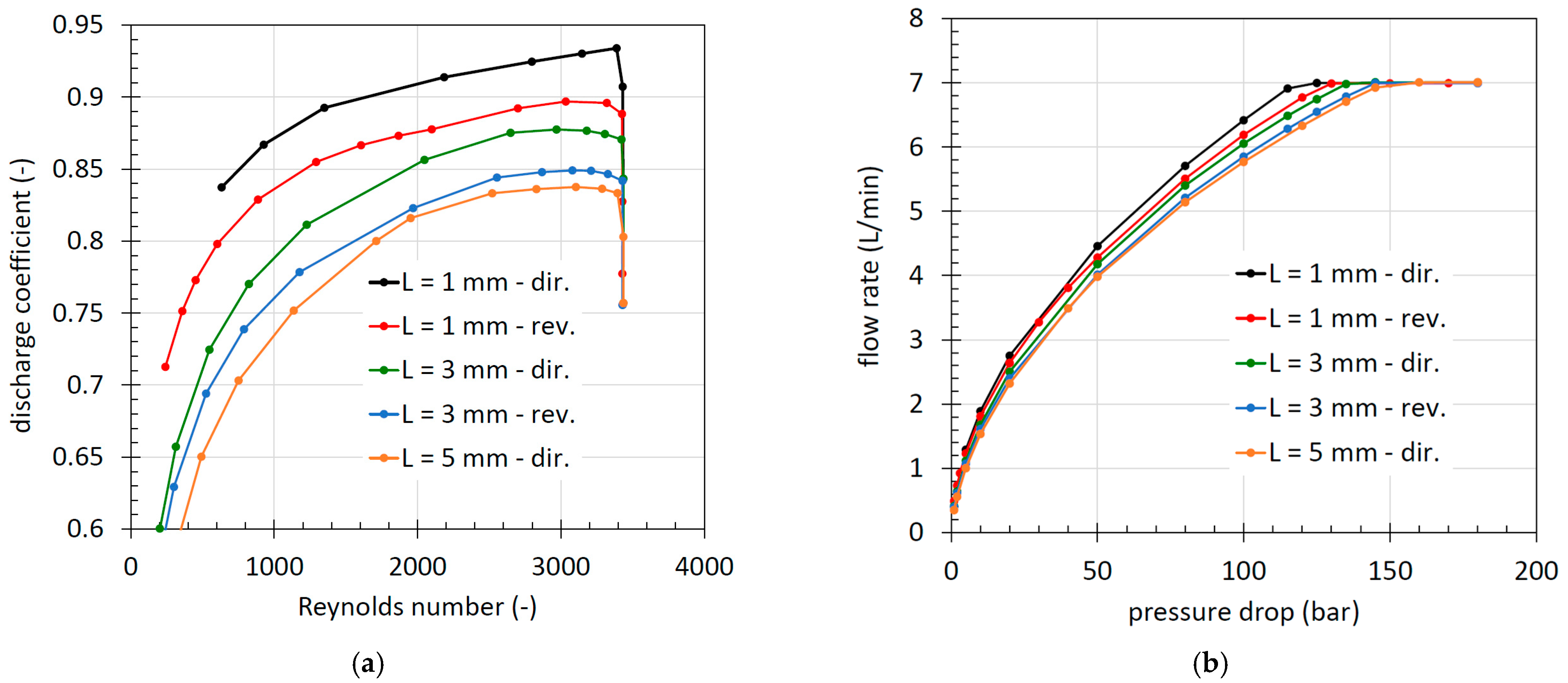
Instead, with reference to the non-cavitating conditions, an approximate analytical expression is provided for calculating C_d to be used in Equation (9) in the specific case of the analyzed geometry (L/D = 1) and for direct flow. The discharge coefficient can be extrapolated from Figure 13b, or for the direct flow, it can be approximated as:

$$C_d=0.4 {Re}^{0.107}$$

(10)

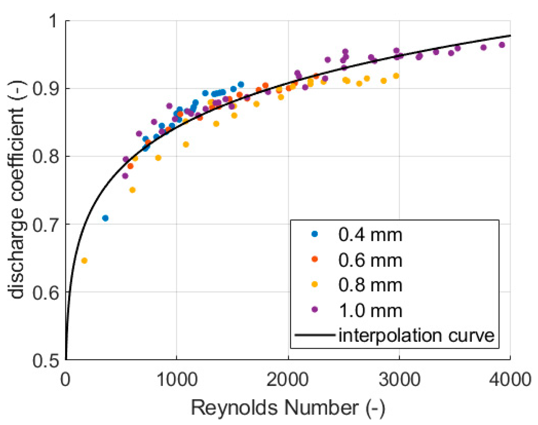
The fitted power law, along with the experimental data points for each orifice diameter, is shown in Figure 21. While achieving a perfect match for every diameter and geometry is not feasible, the proposed analytical model accurately captures the experimental data across all cases with reasonable precision. Statistical analysis of the model indicates a correlation coefficient (R²) of 0.89, a root mean square error (RMSE) of 0.017, and a coefficient of variation (CV) of 78.5%, further validating its robustness.

To demonstrate the accuracy achievable in calculating the flow rate using Equation (10) and the practical implementation in a commercial software package, simulations were conducted in Simcenter Amesim^® Rev 2304. The specific restrictor submodel available in the software, which requires as an input a lookup table that expresses the discharge coefficient as a function of the Reynolds number, was used. This submodel automatically handles the numerical issues of the integrator that would arise when the pressure differential approaches zero [31]. 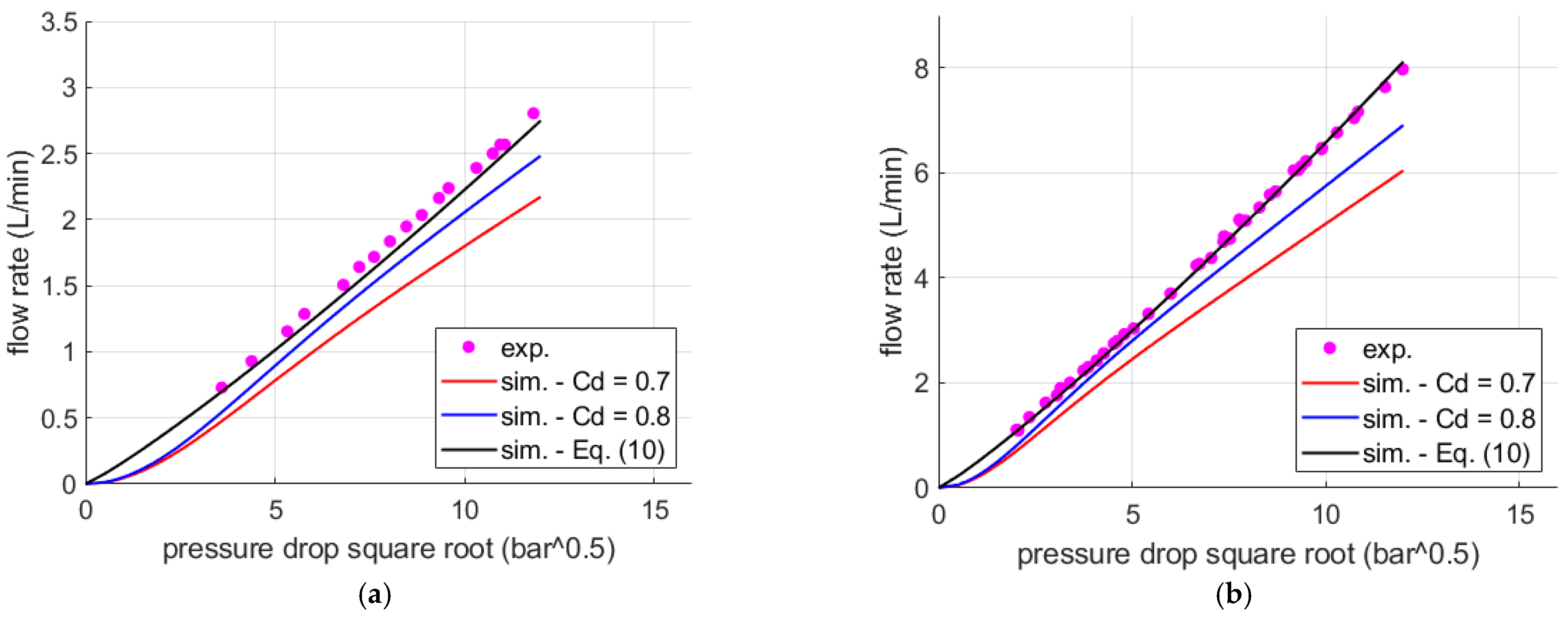Figure 22 reports the flow-pressure drop characteristics for two orifice diameters (0.6 mm and 1 mm), showing both experimental results and simulated data using the lumped parameter model.

The default maximum discharge coefficient value of 0.7, typically used for a fixed orifice in Simcenter Amesim, and an increased value of C_d = 0.8, suggested by the literature [2], are considered for the comparison. In both cases, all other parameters were left at their default values. The simulation results are compared to those obtained using Equation (10).

It can be observed that using the discharge coefficient obtained from the interpolation of experimental data allows for a flow rate that closely matches the measurements. In contrast, the other simulations significantly underpredict the volumetric flow rate, with the discrepancy being more pronounced at lower C_d values. This makes the proposed analytical formulation a valuable tool for modeling orifices with geometries similar to the one studied. It is important to note that factors such as the orifice plate geometry (e.g., sharp edge, chamfered edge), the length-to-diameter ratio, and the direction of flow can significantly influence the discharge coefficient, which in turn affects the derived volumetric flow rate.

6. Conclusions

Prior work has extensively analyzed flow through calibrated orifices and the cavitation phenomenon. However, in the field of hydraulic fluid power components and systems, flow saturation is largely overlooked. This study examines the flow through commercially available screw-in calibrated orifices using hydraulic oil as the working fluid. Through a CFD approach validated experimentally, the discharge coefficient and maximum flow rate for a given upstream pressure were evaluated. It was found that the resistance these orifices impose on the flow is significantly lower than in the ideal case for the same orifice diameter due to the presence of chamfers and the hex wrench socket. However, the maximum flow rate is influenced only by the orifice diameter and is independent of the length-to-diameter ratio. Additionally, it was observed that with hydraulic oil, cavitation occurs at relatively low Reynolds numbers, even before reaching a fully turbulent flow regime. Based on the CFD simulation results, an analytical expression was derived to calculate the flow rate in this specific type of restrictor, also accounting for flow saturation. Finally, an analytical model for deriving the discharge coefficient was presented, which can help improve the accuracy of orifice modeling. Future studies could validate or refine this analytical formulation for operating conditions significantly different from those studied, such as much higher viscosities or very low-pressure drops.