Abstract
Boiling heat transfer plays a crucial role in various engineering applications, requiring accurate numerical modeling to capture phase-change dynamics. This study employs the pseudopotential lattice Boltzmann method (LBM) to simulate boiling heat transfer at different reduced temperatures, aiming to provide deeper insights into bubble dynamics and heat transfer mechanisms. The LBM framework incorporates a multi-relaxation-time approach and the Peng–Robinson equation of state to enhance numerical stability and thermodynamic consistency. Simulations were performed to analyze bubble nucleation, growth, and detachment across varying reduced temperatures, considering the influence of surface wettability, surface tension and gravitational acceleration. The results indicate a strong dependence of bubble behavior on the reduced temperature, affecting both heat flux and boiling regimes. The numerical findings show reasonable agreement with theoretical predictions and experimental trends, validating the effectiveness of the LBM approach for phase-change simulations. Additionally, this study highlights the role of contact angle variation in modifying boiling characteristics, emphasizing the necessity of accurate surface interaction modeling. The outcomes of this work contribute to advancing computational methodologies for boiling heat transfer, supporting improved thermal management in industrial applications.
1. Introduction
The dynamics of multiphase flow is characterized by the concurrent presence of at least two immiscible phases with a dynamic interface connecting them. This interface is the boundary or thin region where two or more distinct phases meet. Physical properties such as density, viscosity, temperature, or composition typically experience a sudden change (or a change in a very small distance) at the interface. The interface thus demarcates the area in which each phase dominates and plays an important role in controlling interfacial phenomena such as surface tension, heat transfer, and mass transfer between the phases. These flow processes occur in many industries, including the extraction and processing of petroleum, conventional and nuclear power, and refrigerator and freezer systems [1,2]. The complexity of multiphase flows stems from the strong interrelationships between fluid dynamics, thermal interaction, mass transfer, and interfacial processes. For example, in boiling, processes such as nucleation, growth, and detachment of bubbles depend on complex interactions between thermal gradients, inertia of the fluid, interfacial tension, and kinetics of transition between phases [3]. Consequently, simulations that seek to accurately model multiphase flows, and specifically boiling heat transfer, require much larger computational capabilities compared to their single-phase counterparts. Therefore, sophisticated numerical methodologies are required capable of tracking interfaces and accurately simulating localized conduction and convection processes.
Bubble nucleation on heated surfaces forms the foundation of many engineering applications, especially in boiling processes within flooded evaporators commonly used in vapor-compression refrigeration systems [3]. Boiling, with its high thermal conductance, has been a well-examined phenomenon for many years. An early experimental investigation by Nukiyama [4] developed the concept of the boiling curve, a relation between heat flux and wall superheat in pool boiling, defining operational regimes through its nonmonotonic behavior (e.g., Figure 1): natural convection, nucleate boiling, transition boiling, and film boiling. Notably, Nukiyama also documented a hysteresis between nucleate and film boiling, characterizing complex behavior in phase-change thermal conduction. Following Nukiyama’s work, numerous experimental studies have continued to develop a deeper understanding of the laws governing boiling thermal conduction through its constituent processes, including bubble growth, detachment, and coalescence, over a full range of operational scenarios and surface character [5,6,7].
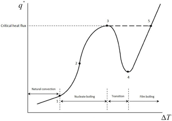
Figure 1.
Schematic representation of the boiling curve: 1—onset of nucleate boiling, 2—fully developed nucleate boiling, 3—critical heat flux, 4—transition, 5—film boiling.
Concerning nucleate boiling, the processes involved in heat transfer responsible for high heat transfer coefficients include the following:
- Microlayer evaporation underneath a bubble.
- Transient conduction in overheated liquid.
- Convective transport caused through bubble motion.
- Surface rewetting and bubble pumping effect.
In recent years, computational approaches have increasingly been adopted as complementary approaches to experimental testing in Thermal and Fluids Engineering. Behind this development, for the most part, have been both commercial (e.g., ANSYS Fluent, COMSOL) and free-access simulation software (e.g., OpenFOAM), allowing for simulation of complex flow behavior under a range of working conditions [8].
A key challenge in Computational Fluid Dynamics (CFD) is an accurate simulation of multi-phase flows, for which techniques such as the Volume of Fluid (VOF) and Level Set (LS) approaches have become widespread practice. These techniques rely on continuum hypotheses and solve Navier–Stokes equations (in conjunction with energy and species conservation equations when applicable) over a computational region of interest. Next, an additional transport equation is added in order to track the motion of an interface. For the VOF method, a color function or a function of a volume fraction describes phases of a fluid, whereas in the Level Set method, a signed distance function is utilized in determination of an interface location [9]. Both approaches involve incorporation of surface tension forces through specific formulations such as with the Continuum Surface Force (CSF) model [10] and require careful processing of an interface reconstruction in an attempt to avoid numerical diffusion.
Although continuum models can work for a variety of engineering scenarios, specific processes such as near-wall microphysical behavior, events of a phase transition, and interfacial microstructure could use a less phenomenologic basis for a model. In principle, microscopical techniques such as Molecular Dynamics (MD) and Direct Simulation Monte Carlo (DSMC) bypass continuum approximation through direct resolution of Newton’s laws of motion for discrete particles and molecules, respectively. However, these techniques demand high computational capacities, even with ongoing improvements in high-performance computers [11,12,13].
Mesoscopic methods represent an attractive intermediate between purely continuum and purely molecular representations, and LBM is the most exemplary of them. The method works with the Boltzmann transport equation over a discrete lattice structure, allowing for efficient simulation of interfacial behavior and phase transformation processes at a level of detail unnecessary for conventional continuum solvers [11]. In a modern development, complex numerical methodologies, including LBM, have been developed for simulations of multiphase flows with interfacial behavior [7,14]. LBM-inspired approaches allow for in-depth analysis of bubble development, growth, and disengagement over hot walls, supporting improvements in thermal system design and thermal performance optimization through boiling processes [15,16].
In recent years, the LBM with a pseudopotential model has proven a viable alternative for conventional CFD approaches for the simulation of multiphase and phase-change behavior, specifically in complex thermofluid problems in which careful tracking of interfaces is critical [17,18]. Rooted in the Kinetic Theory of Gases, the LBM describes fluid dynamics at a mesoscopic level through distribution functions for particles defined in a discrete velocity set. By utilizing density gradients in distribution functions, the LBM naturally accommodates interfaces, circumventing explicit tracking techniques that mark conventional CFD approaches [11].
A significant advantage of the pseudopotential LBM for boiling heat and similar phase-change processes stems from its ability to calculate pressure directly through an Equation of State (EOS), first developed by Shan and Chen [17]. In so doing, a Poisson equation is avoided, and overall computational requirements are reduced, a feature not necessarily linked with pressure–velocity coupling in conventional CFD solvers. In addition, the LBM’s native localized updating processes make it even more apt for parallelization, increasingly critical with high-performance computer availability becoming widespread.
Notwithstanding these strengths, it must be acknowledged that the LBM with a pseudopotential model is explicit in time; therefore, taking smaller time steps in an attempt to maintain numerical accuracy and stability will drive overall computational cost higher. In addition, in contrast to conventional CFD, requirements for resolution and grid density can become even more extreme in an attempt to accurately represent interfacial behavior, yet at a cost in computational efficiency. Existing work is focused towards developing hybrid approaches and optimized collision processes to mitigate such weaknesses, yet all in an attempt to maintain inbuilt capabilities for representing interfaces and proving strong performance in modern parallel computer architectures [19,20].
Among the many forms of LBM approaches, the pseudopotential model has become increasingly popular in two-phase and multiphase flow simulations. According to [21], such a scheme proves computationally efficient over a wide range of multiphase problems but can face numerical instabilities when dealing with low density and high density-ratio scenarios in its application. Consequently, several improvements have been proposed for enhancing both its accuracy and stability. For one, the authors of [22] analyzed and optimized the early pseudopotential model for spurious current elimination, terms for such current appearing in terms of nonphysical velocity gradients at interfaces between phases in contact with one another. In follow-up studies. the authors of [23] derived an extended expression for a pressure tensor, allowing for a more sophisticated integration of inter-molecular forces between adjacent lattice nodes. With such an optimized configuration of a pressure tensor, one can effectively reduce spurious interfacial current, allowing for two-phase simulations over a broader range of flow regimes compared with a traditional Shan–Chen model.
Numerous studies have utilized the LBM for studying boiling behavior, bubble growth, and nucleation over boiling-promoting surfaces, with many of them utilizing the pseudopotential model [17,18]. Most of them, however, depend on idealized and restricted conditions, not closely resembling simulation parameters and experimental data for specific fluids collected in actual experiments. This model enables a better simulation of underlying processes, most notably in relation to bubble development and growth over boiling-promoted surfaces. The LBM holds several key advantages in such a use, such as a relatively simple development process and its intrinsic ability to simulate interfaces between phases—advantages not easily obtainable with conventional computational fluid dynamics simulations reliant on sophisticated interface tracking and rebuilding techniques.
The pseudopotential model, as explained by [24], is the most common multiphase LBM used in simulations of vapor–liquid phase transitions associated with heat transfer mechanisms. The model has been widely used to study a range of one-component liquid–gas two-phase phenomena, which include stationary droplet evaporation, nucleate pool boiling in cavities and channels [25,26,27,28], flow boiling [29,30,31], gas–liquid condensation [32], and cavitation [33], as well as other related phenomena.
Early work by [34] demonstrated that coupling hydrodynamic and thermal fields via an equation of state could effectively model bubble departure characteristics, matching empirical gravity-based predictions. Later, ref. [35] incorporated the energy equation directly into the LBM using an additional temperature distribution function, though this approach led to some asymmetries in the flow field. Based on these studies, ref. [36] introduced a modified pseudopotential LBM with a new source-term formulation to resolve previous inconsistencies, which yields improved stability, accuracy, and computational efficiency compared to traditional CFD methods. Finally, subsequent studies by [37,38] extended the model to investigate the role of surface wettability, revealing distinct bubble dynamics on hydrophilic versus hydrophobic surfaces and successfully capturing various boiling regimes within a single boiling curve.
Recent advances in color-gradient multiple-relaxation-time (MRT) lattice Boltzmann models have significantly improved the simulation of two-phase flows with high density ratios and complex interfacial phenomena [39,40,41]. These studies emphasize the importance of accurately capturing surface tension and contact angle behavior, both of which critically impact droplet formation, breakup, and coalescence. In [39], a novel MRT-based color-gradient framework demonstrates stronger stability and reduced spurious currents compared to single-relaxation-time approaches, while [40] extends these ideas to more complex Multiphysics problems by refining the collision operator and force modeling for better interface morphology representation. Complementarily, ref. [41] highlights the capability of color-gradient models to handle boiling and phase-change processes, providing accurate depictions of bubble nucleation and detachment in high-density-ratio scenarios and confirming the broader applicability of MRT-based color-gradient LBM schemes in tackling intricate two-phase flow challenges.
Realizing the importance of accurately simulating boiling heat transfer and the intricacies involved with interface tracking in phase-change problems, this study aims to expand the application of the pseudopotential lattice Boltzmann method (LBM) for the study of boiling dynamics at different reduced temperatures. The primary objectives are to investigate the influence of reduced temperature on bubble nucleation, growth, and detachment to assess the impact of surface wettability on boiling regimes and to validate the numerical model by comparison with theoretical predictions. Through the implementation of a multi-relaxation-time approach in combination with a Peng–Robinson equation of state, this study aims to improve the stability and accuracy of the LBM in simulating phenomena related to phase changes. The insights gained from this research contribute to the advancement of computational methods for boiling heat transfer, hence enabling the development of more efficient thermal management strategies in industrial applications.
2. Numerical Model
The formulations of the equations utilized in the numerical model via the MRT operator are presented herein and combined from the formulations presented in [42,43]. The method maintains thermodynamic consistency and allows for independent variation of the surface tension with respect to the density ratio, which forms a viable foundation for simulating multiphase phenomena of boiling heat transfer accurately.
The energy equation is discretized in space with a Finite Difference Method (FDM) and approximated in time with a fourth-order Runge–Kutta scheme. In this manner, a high level of accuracy in both the space and time dimensions is attained. Appropriate boundary and initial conditions are determined to accurately simulate real boundary and initial conditions in boiling processes, such as wall temperatures, fluxes, and thermal property values at interfaces in a fluid. Next, a general expression for boundary and initial conditions is derived, together with a consideration of its stability, convergence, and its integration with a base lattice Boltzmann solver for simulations in phase change [13].
2.1. Hydrodynamic Sub-Model
The hydrodynamic sub-model applies the multi-relaxation-time (MRT) approach within the context of the lattice Boltzmann equation, thereby handling streaming and collisions within a moment space rather than directly in distribution-function space. The discrete evolution of the density distribution function is represented by
The matrix serves as an orthogonal transformation that links distribution functions to a desired set of moments. This mapping facilitates the independent relaxation of each moment via a diagonal relaxation matrix, , containing all the relaxation times. The relaxation rates are carefully selected to enhance numerical stability and accuracy, especially in comparison to a single-relaxation-time approach, and are particularly beneficial in simulations with high-gradient conditions typical of boiling heat transfer.
The discretized form of the equilibrium distribution function can be expressed as
where is a constant, namely the speed of sound, which is a function of the chosen velocity scheme; is the fluid macroscopic velocity; and is the fluid density.
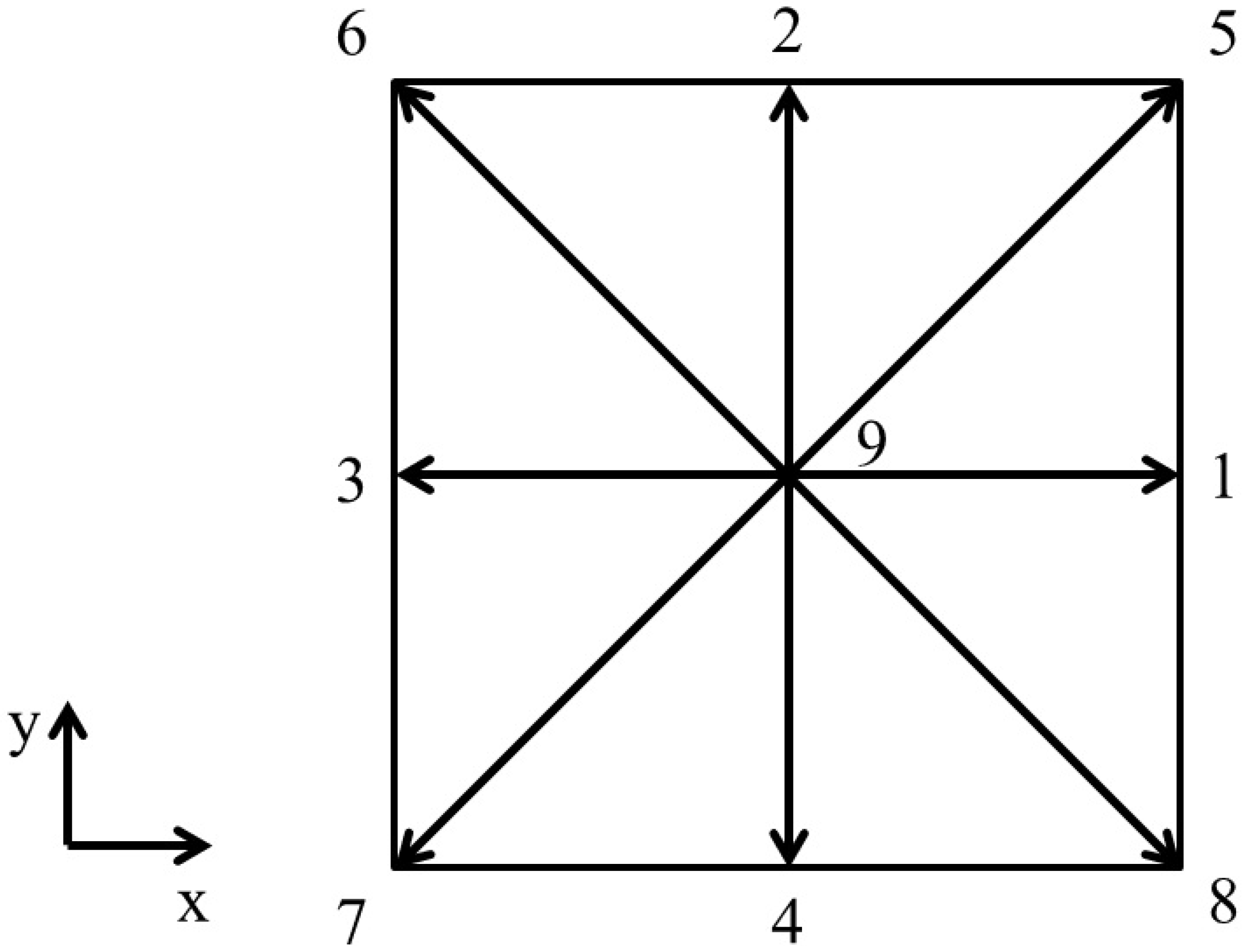
The two-dimensional numerical simulations utilize the D2Q9 velocity model. Figure 2 depicts a diagram of this scheme.

Figure 2.
Schematic representation of D2Q9 discrete velocity scheme (D2 indicates a two-dimensional simulation domain and Q9 indicates that each lattice site has nine discrete velocity directions, indicated using values 1 to 9).
For this velocity scheme, the speed of sound is . Also, for this velocity scheme, the weighing coefficients, , and the discrete velocities, , are given by, respectively,
The transformation matrix M for the D2Q9 model is given by
The revised external forcing approach described in [42] is included to maintain thermodynamic consistency within the phase change model. To accurately depict interfacial dynamics, surface tension follows the strategy outlined in [43]. In the context of the multi-relaxation-time (MRT) model, collisions occur within the moment space. The moments produced during a collision are mathematically derived from the previous moments, as demonstrated in Equation (6):
The streaming operation is carried out in velocity space, using Equation (7).
where , , is the unitary tensor, and is the forcing term in the moment space with .
The diagonal matrix is given by [44]
where and are the relaxation parameters of conserved moments and are set to 1, determines the dynamic viscosity, is associated with the bulk viscosity and is set to 1.1, is related to energy square and is set to 1.1, and is related to the energy flux and is set to 1.1.
From , the equilibrium momentum can be expressed as
where .
To maintain thermodynamic consistency, the forcing scheme developed by [42] is used, which involves adjusting the mechanical stability condition. In this framework, the forcing term is defined as follows:
where is a parameter used to tune the mechanical stability condition; , is the total force; , where and are the total force components; and and are the fluid velocity components.
In the model proposed by [43], the additional source term has the following form:
where the terms , , and are computed as described in Equation (12):
where is a parameter that allows a tunable surface tension and are the redefined weight functions [15].
Based on [45], the pseudopotential function is calculated from a non-ideal equation of state:
The Peng–Robinson equation of state is used to calculate the pseudopotential, according to Equation (13):
When the pseudopotential is calculated by Equation (13), it is found that the intermolecular interaction force becomes independent of the parameter G. In this case, G is used only to ensure that the square root of is always positive.
The intermolecular interaction force is computed according to Equation (15):
Apart from this intermolecular interaction force, there are other forces involved in the bubble formation on heated surfaces problem to be incorporated in the hydrodynamic model. The buoyancy force is introduced as in [45], using Equation (16):
In Equation (16), g represents the acceleration due to gravity, and denotes the average density computed accounting for the entire computational domain. Implementation of the buoyancy force in this form is most commonly found in the literature since it ensures that the acceleration of the system is zero [46].
The interaction force between the solid surface and the fluid, used to adjust the contact angle, is introduced according to [19] by Equation (17):
In Equation (17), is a parameter that represents the magnitude of the interaction between the fluid and the solid in order to adjust contact angles, and is a function that is unity if the position corresponds to the solid and null otherwise.
The density and velocity fields are obtained directly from the distribution function, , through Equations (18) and (19), considering the effect of the total force , respectively:
For the model used, the solved hydrodynamic equations obtained through the Chapman–Enskog Expansion are expressed by [19]:
In Equation (21), it is noted that the effects of the buoyancy forces and the surface interaction force appear explicitly. The intermolecular interaction force is introduced through the pressure tensor. For the model used in this paper, the pressure tensor according to [42,43] is the following:
2.2. Thermal Sub-Model
Following the approach introduced by [19], the numerical solution of the energy equation is based on the fourth-order Runge–Kutta method. This is justified by the fact that when using the lattice Boltzmann method to solve this equation, the source term must still be discretized by finite differences. Thus, through the temporal integration of the Equation (23) by the fourth-order Runge–Kutta method, the temperature at the next instant of time is calculated by
It should be noted that the diffusive term was expanded according to .
2.3. Boundary Conditions
For the hydrodynamic model, the boundary conditions are given in terms of the distribution function. In this work, the boundary conditions considered by [19] will be used. In this case, the lower and upper surfaces will be modeled as solid walls at rest and for the lateral surfaces, periodic boundary conditions are considered. Considering the latter, it is assumed that the computational domain has a sufficiently large dimension in this direction. Periodic boundary conditions are easily applied by means of an appropriate numerical implementation of the streaming operation.
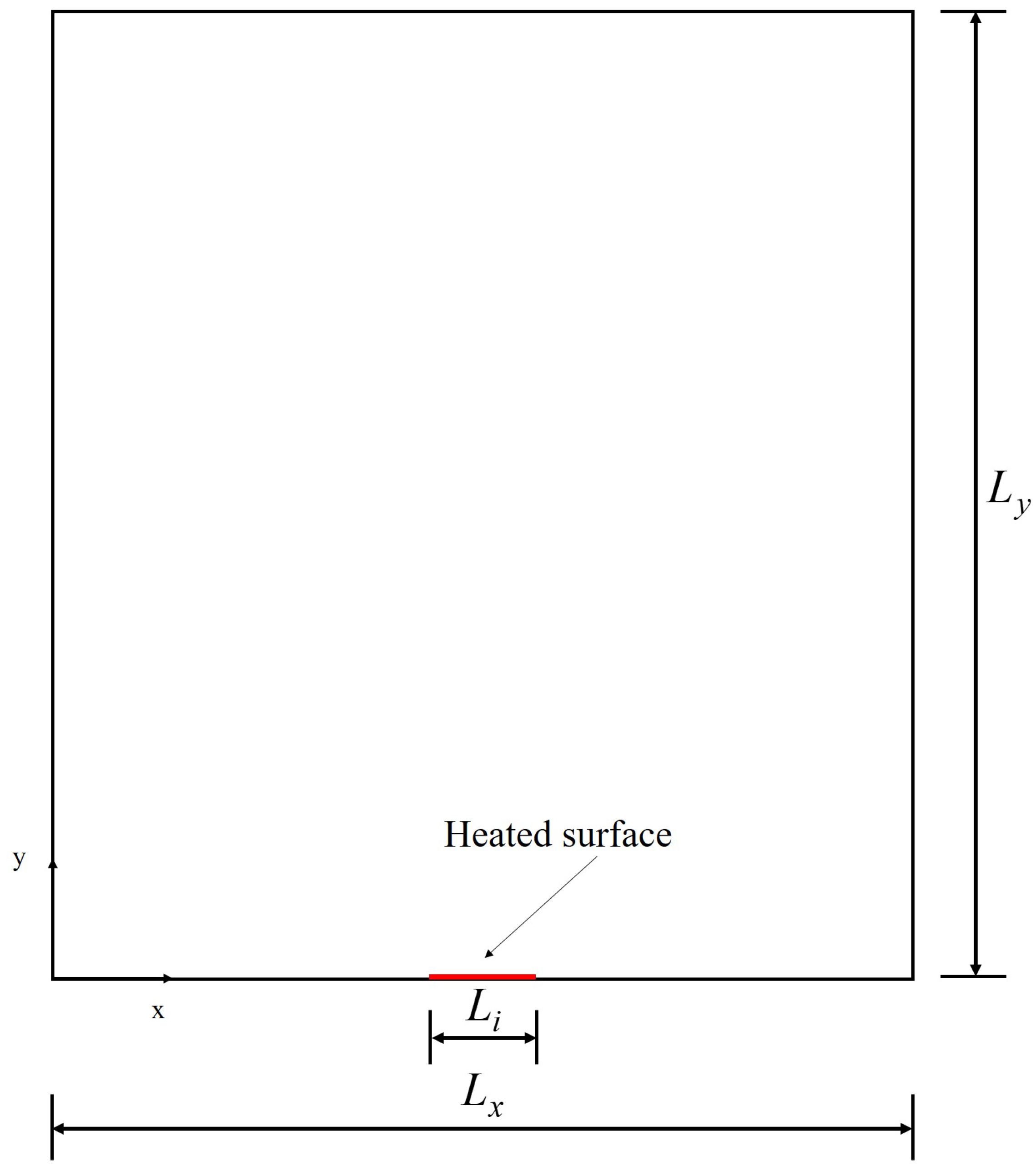
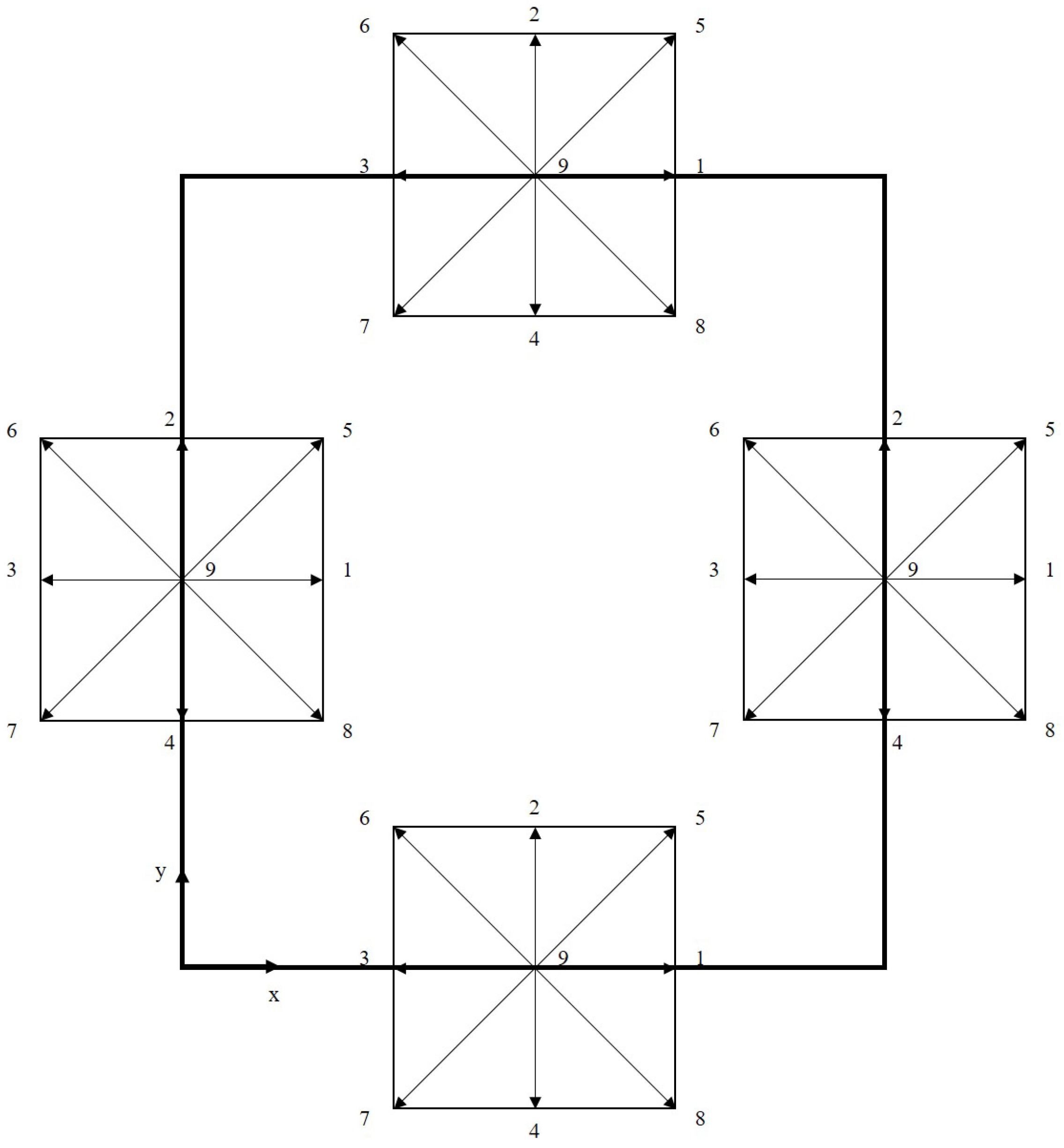
A schematic representation of the computational domain is shown in Figure 3, with dimensions and , including the heating surface. Considering the velocity scheme , used to perform the simulations, and the domain represented by Figure 3, it follows that, after the transmission operation (streaming), the distribution functions with directions towards the interior of the computational domain must be determined, as shown in Figure 4.

Figure 3.
Schematic representation of the computational domain.
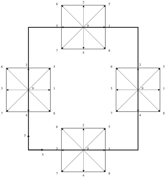
Figure 4.
Schematic of the boundary conditions for the D2Q9 velocity scheme (D2 indicates a two-dimensional simulation domain and Q9 indicates that each lattice site has nine discrete velocity directions, indicated using values 1 to 9).
For the left lateral surface (), the periodic boundary condition is expressed by the following relation, considering the directions :
For the right lateral surface (), the periodic boundary condition is expressed by the following relation, considering the directions :
The condition at the fluid–solid interface applied in this paper is the no-slip condition. In the lattice Boltzmann method, this boundary condition can be implemented by means of the bounce-back scheme [48].
The bounce-back scheme is based on the condition that, during the transmission stage, the populations that reach the wall are reflected in the direction of the domain. In this way, the normal and tangential components of the velocity are reversed.
The formulation in terms of the distribution function for the bounce-back boundary condition is based on equating the unknown distribution functions to the opposite distribution functions at the fluid–solid interface. Considering the discretization scheme in velocity space , the following relation should be applied [11]:
Another scheme that allows the implementation of the no-slip condition was proposed by [49]. In this work, the authors developed a general scheme for solid walls with a given velocity, . This is the scheme adopted in this work. For simplicity, the distribution function will be presented simply by , omitting the argument . Assuming that the lower solid wall has density (to be calculated), velocity given by and initially disregarding the effect of external forces, the following relations can be obtained, considering Equations (18) and (19):
However, the components in the 2, 5, and 6 directions are unknown. The closure of the system of equations is based on admitting that the bounce-back rule is applied to the non-equilibrium portion () of the function distribution in the normal, 2, and 4 directions:
In this way, equations for the unknown directions can be obtained:
An analogous procedure can be obtained for the upper boundary so that the density at the boundary and the distribution functions of the unknown directions can be obtained:
The effect of external forces on the calculation of the distribution function at the lower and upper boundaries is now considered. According to [11], by the Chapman–Enskog expansion for the upper boundary under the effect of forces, Equations (44)–(46) are modified and the equations to be applied are given by
Similarly, for the lower boundary, the equations that allow the calculation of the density at the wall and the unknown distribution functions are given by
It is worth noting that, for the particular case of the simulations carried out in this paper, the velocities of the solid walls are zero, so that .
Unlike the hydrodynamic model, for the thermal model the boundary conditions are expressed directly in the temperature field, since the fourth-order Runge–Kutta method is used.
For the temperature field, one can basically consider Dirichlet (constant temperature) or Neumann (constant heat flux) boundary conditions. For the first case, the evolutionary equation for temperature (Equation (23)) is solved for the nodes inside the domain and the boundaries have a known temperature. For the second case, the temperatures at the boundaries can be extrapolated considering the interior nodes, and the temperature at time is obtained by Equation (23), as indicated in [24].
For the constant temperature condition, the upper and lower boundaries are considered to have temperatures equal to the saturation temperature. For the constant heat flux condition, the upper and lower surfaces are considered adiabatic. For both conditions, it is assumed that the heating surface has a constant temperature, given by .
2.4. Initial Conditions
For bubble cycle simulations, the density field is imposed as a liquid–vapor mixture, with each phase occupying of the computational domain [20]. For simulations of the boiling curve, the density field is imposed as a liquid–vapor mixture, with each vapor occupying of the computational domain and the liquid phase occupying the remainder [19]. For both cases, the initial velocity field is assumed to be zero [20].
As an initial condition for the hydrodynamic model, typically in the literature, the equilibrium distribution function is used as an initial condition, as follows:
In this work, a different strategy is used, based on the work of [50,51]. In this case, once the initial density and velocity fields are known, the equilibrium distribution function is calculated and used in the initialization. Subsequently, only the hydrodynamic model is solved, without the effect of gravitational acceleration, until the density and velocity fields reach convergence, considering a relative residual of . After the fields converge, the effect of gravitational acceleration is considered and the energy conservation equation is solved.
For the thermal model, the initial condition is imposed assuming an uniform temperature in the computational domain and equal to the saturation temperature: .
3. Results and Discussion
This section presents numerical results obtained by implementing and simulating bubble formation on heated surfaces using the lattice Boltzmann pseudopotential method. The simulations are performed with parameters from the literature. Thus, the variables used are presented in lattice units, in the same way as other works in the literature [15,19,36,37,38,52].
For all simulations, the relaxation frequencies were chosen according to the work of [42]: , . Relaxation frequencies and are calculated from kinematic viscosities.
As some of the results are presented in the dimensionless form, proper scales need to be defined. Taking into account the work of [53], the length scales , velocity , and time scales are defined as
All simulations were performed on a desktop computer with an Intel® Core i7-4790 CPU @ 3.60 GHz x 8, with 32 GB of RAM (Intel Corporation, Santa Clara, CA, USA). The computational code was implemented in software MATLAB® R2022b.
3.1. Simulation of a Bubble Cycle Using Literature Data
In this section, the bubble cycle simulations use the parameters described in the study by [20]. The simulations were conducted for a reduced temperature of . For the Peng–Robinson equation, the parameters are set as , , and . This allows us to determine the critical temperature, which is . The equilibrium density values are and . Thermophysical properties include , , and . It is important to note that both phases were assigned the same value for thermal diffusivity. The thermal conductivity for each phase is determined by , as outlined in [20]. Furthermore, the authors assumed . The acentric factor corresponds to that of water, namely . Lastly, the thermodynamic consistency adjustment parameter is set to .
Using the provided data, the initial step involves determining the surface tension by simulating a hydrodynamic scenario involving a static drop surrounded by its vapor phase. The computational grid used is 200 by 200, with periodic boundary conditions enforced in every direction. The parameter , used to modulate the surface tension, is initially set to . Under these conditions, the temperature remains constant at the saturation point. To shape a circular liquid drop, the density distribution is defined as follows [21]:
With reference to the parameters of Equation (59), represents the initial droplet radius, denotes the center coordinates of the computational domain, and indicates the thickness of the interface as per [15]. The simulation convergence criterion is established by assessing the relative error in the density field in successive iterations, with a residual value set to . Once the density field has converged, the surface tension is calculated using the Young–Laplace equation:
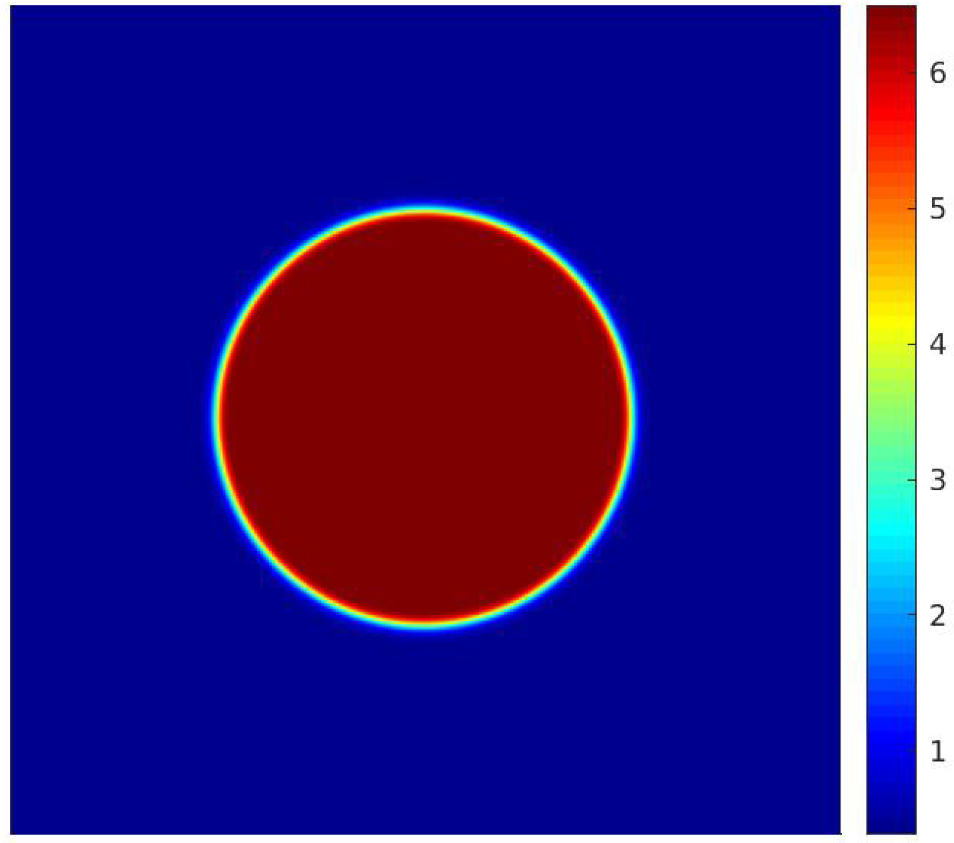
In Equation (60), represents the pressure differential across the droplet, denotes the surface tension, and is the droplet’s radius. It is important to mention that the equilibrium radius of the droplet post-simulation convergence could differ slightly from its initial radius, . Consequently, once the simulation converges, the droplet radius is recalculated using a numerical method, with the interface defined at the point where , according to [11]. Figure 5 presents the density field achieved after the simulation has converged.
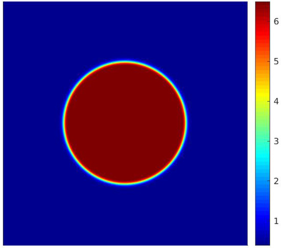
Figure 5.
Density field for considering the input data from [20].
For the parameters of the work of [20], the surface tension calculated by simulation for the model with the MRT operator is equal to , a value obtained for . For the simulation of bubble formation, the upper and lower surfaces are modeled as adiabatic solid walls (except for the heating surface), and periodic boundary conditions are assumed on the side walls. The heating surface is located at the center of the lower wall and has length , being formed by the central node and the adjacent nodes to the left and right. The temperature of the heating surface is constant and equal to . The computational mesh used for the simulations is 150 × 300, the same as adopted by [20]. The adjustment parameter for the contact angle is chosen as so that the contact angle is approximately equal to 45°.
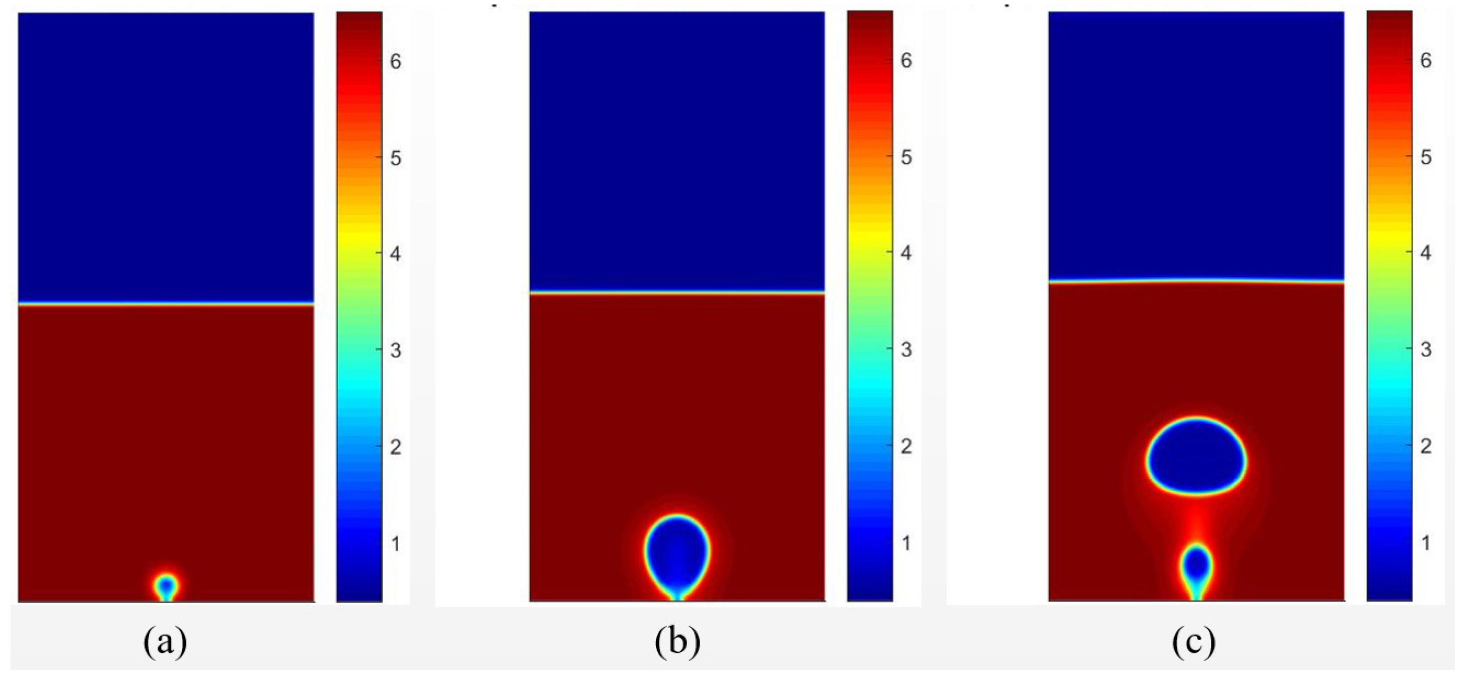
Figure 6 presents the results of the density field for different time intervals for the condition in which . The temperature field for the same instants is presented in Figure 7. It is possible to observe the formation of a vapor nucleus near the heating surface because of the higher temperature. After , bubble detachment is noted due to the effect of buoyancy force.

Figure 6.
Results of the density fields obtained with data from [20], considering for different time periods of (a) , (b) , (c) .

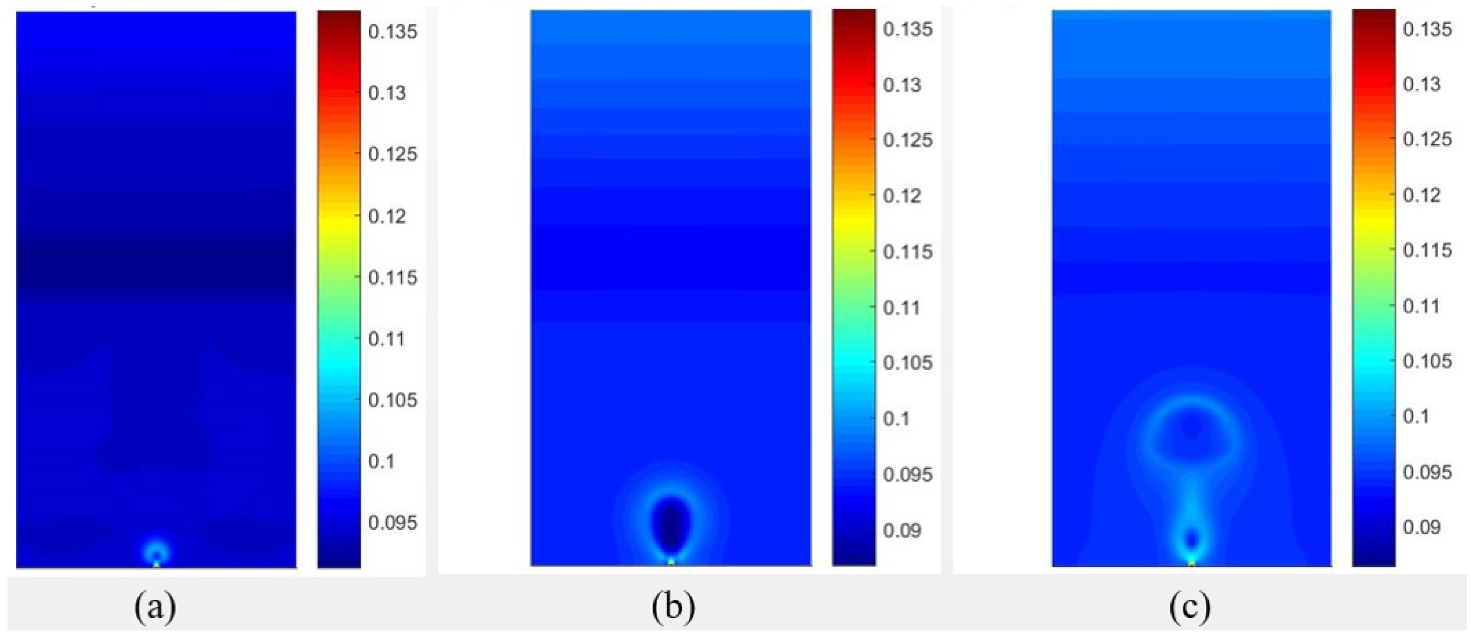
Figure 7.
Results of the temperature fields obtained with data from [20], considering for different time periods of (a) , (b) , (c) .
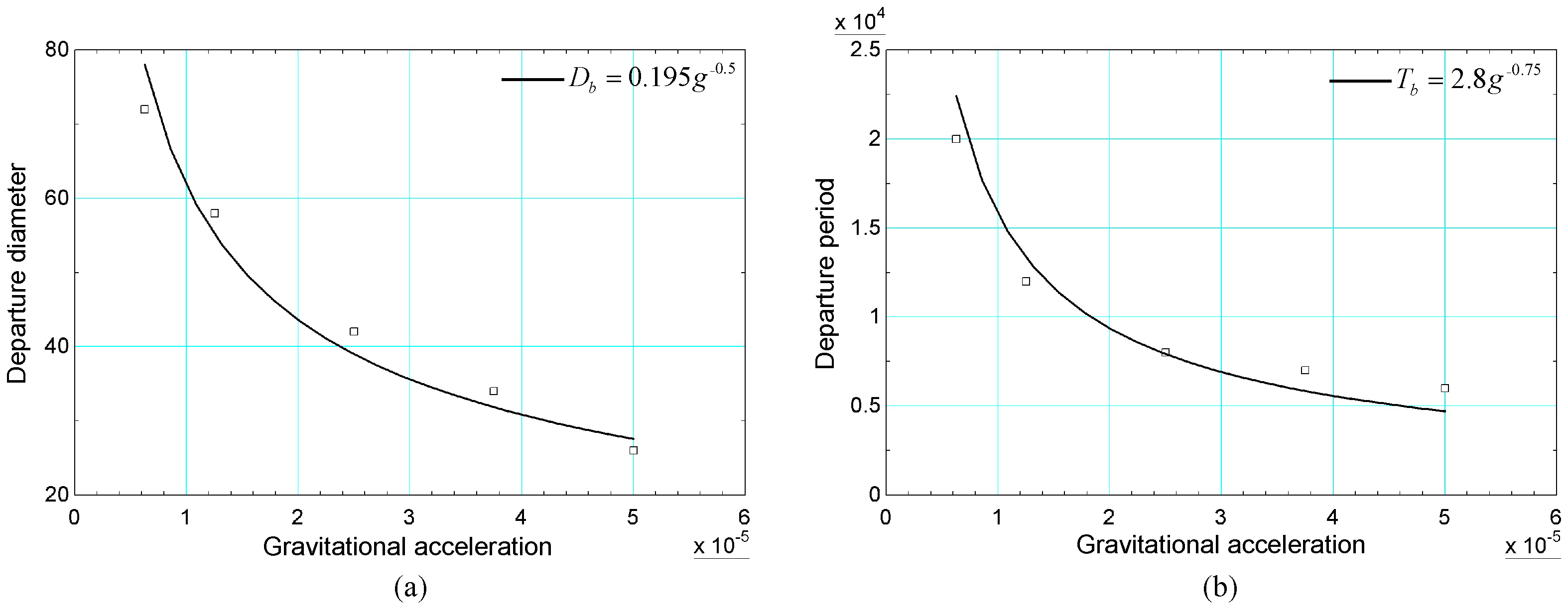
From a theoretical point of view, the increase in gravitational acceleration results in a smaller diameter and shorter detachment period. This is justified by the increase in the buoyancy force, which favors the detachment of the bubble from the heated surface. Simulations of the bubble cycle were performed for different values of gravitational acceleration, starting from to , with uniform increments. The numerical results of the diameter and detachment period were obtained and are presented in Figure 8. In addition, fitted curves of the relationships are considered based on the diameter and detachment period considering the correlations of [54,55]. These correlations are given, respectively, by Equations (61) and (62):
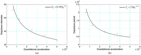
Figure 8.
Results of (a) diameter and (b) bubble detachment period versus gravity acceleration obtained with data from [20].
Taking into account these correlations, the relationships between the diameter and the period of detachment with the gravitational acceleration are, respectively, and . It is noted that the numerical results are in reasonable agreement with the previous relationships.
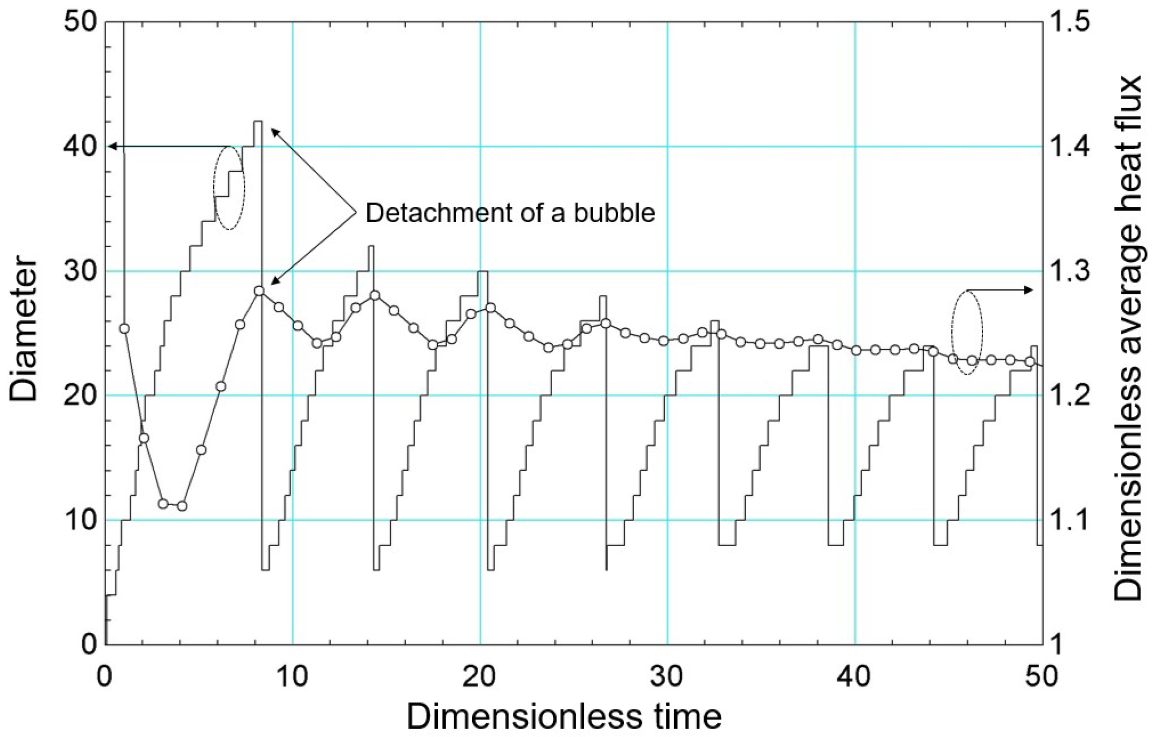
During the bubble cycle, the dynamic behavior of the spatial-averaged heat flux allows the definition of the bubble expansion and liquid wettability processes. For the first process, the effect of bubble expansion results in a reduction in the spatial averaged heat flux. For the second, the effect of liquid wettability results in an increase in the heat flux. The spatial-averaged heat flux can be defined by the following relation:
In Equation (63), the wall temperature gradient is calculated using a second-order finite difference approximation.
The transient average spatial heat flux, in dimensionless form, can be expressed considering the formulation introduced by [26]:
In Equation (64), the enthalpy of vaporization, , is calculated according to the procedure of [52] based on the definition of enthalpy given by Equation (65):
In Equation (65), p is the pressure calculated using the non-ideal equation of state.
Considering the Peng–Robinson equation of state, the resulting equation for calculating enthalpy is given by
In Equation (66), . Therefore, the enthalpy of vaporization can be calculated by .
Figure 9 shows the diameter and the dimensionless area-averaged heat flux versus dimensionless time (dimensionless through the time scale, , given by Equation (58)) during the bubble cycle. For the first cycle, which is the longest compared to the others, there is a reduction in the heat flux to , which corresponds to the bubble expansion process. From this moment on, the heat flux begins to increase, characterizing the liquid wettability process. The peak of the heat flux corresponds to the moment the bubble detaches from the heated surface.
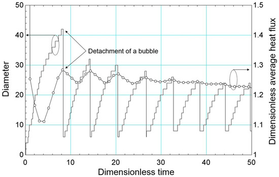
Figure 9.
Bubble diameter results and dimensionless area-averaged heat flow versus dimensionless time.
After carrying out a preliminary comparison with empirical results, more specifically the diameter and frequency of detachment, the numerical model can be used for parametric analyses, as well as comparison of different models.
3.2. Simulation of the Boiling Curve Using Literature Data for Different Reduced Temperatures
The pseudopotential method was applied in the literature to simulate the boiling curve. In this case, it is considered that the heating surface corresponds to the entire lower surface, that is, according to Figure 3. In this section, different reduced temperatures were considered and a qualitative comparison between the results was performed considering the parameters of the works of [19,26].
In the work of [19], the different regimes of the boiling curve were simulated for different liquid wettability conditions. The simulations were performed again for , whose equilibrium densities were used in the previous section. The following parameters were used: , , , and . From the last relation, it is observed that the authors related the thermal diffusivity to the specific heat at a constant volume, which differs from the definition: . Thus, it is concluded that the authors considered .
In the work of [26], the simulations of the boiling curve were performed at . The Peng–Robinson equation of state was used, considering the parameter . In order to obtain the same critical temperature for both reduced temperatures, the parameter a of the equation of state was chosen as . Considering , it follows that the critical temperature is the same for both conditions. For , the equilibrium densities are and . The viscosities of the phases are . The thermal diffusivities are and . Finally, the specific heats used were and .
For all thermophysical properties used, the same interpolation scheme given by Equation (67) is applied:
The acentric factor is that of water: . The thermodynamic consistency adjustment parameter is the same as in the previous section: . The gravitational acceleration was assumed to be for both cases, as well as the computational mesh: 600 × 150. The contact angle adjustment parameter was assumed to be , resulting in a contact angle of °. Solid wall boundary conditions with constant temperature were assumed for the lower and upper surfaces, while periodic boundary conditions were assumed for the lateral surfaces. On the lower surface, the temperature is given by , where is the surface superheating. The upper wall has a constant temperature and is equal to the saturation temperature, . These same boundary conditions were considered by [19].
In the work of [19], temperature fluctuations were inserted into the equation of state used in the calculation of the pseudopotential (Equation (13)) in order to intensify the formation of bubbles on the surface. These fluctuations are necessary since the superheating is applied across the entire heating surface. In this work, the temperature fluctuation introduced into the pseudopotential is applied at the center of the computational domain and was considered equal to half the critical temperature calculated previously.
The methodology used by [19] for numerical simulations for different values of surface superheat is described below. The authors defined, through simulations, that the onset of boiling (ONB, onset of nucleate Boiling) occurs for . For simulations with higher superheats, the authors simulated 20,000 instants for and, from that instant on, a new value for surface superheat was used. Regarding the work of [26], it is noted that surface superheat is used from the beginning of the simulations, that is, in a different way to the procedure adopted by [19]. In this paper, it was decided to carry out the simulations in the same way as [26], that is, using the desired superheating from the beginning of the simulation.
At this point, a discussion regarding the non-dimensionalization of surface superheating is carried out as follows. In the work of [26], the authors non-dimensionalized the surface superheating by means of the Jakob number. However, based on the literature review carried out in this paper, it is noted that the choice for the specific heat in lattice units appears to be by numerical experimentation. On the other hand, in the work of [19], the authors presented all the results of average heat flux versus surface superheat in lattice units.
In this paper, we chose dimensionless space-averaged heat flux and surface superheating using parameters that can be obtained through the equation of state and the saturation temperature. This is justified by the fact that the value of the specific heat used in the mentioned works was not obtained as a function of the temperature (as performed in the international system of units). Thus, we propose to make dimensionless the surface superheating according to the Equation (68):
After calculating the spatial-average heat flux using Equation (63), the temporal average is performed using Equation (69):
where is the total simulation time. The simulation is performed until the spatially averaged heat flux remains constant among 1000 iterations.
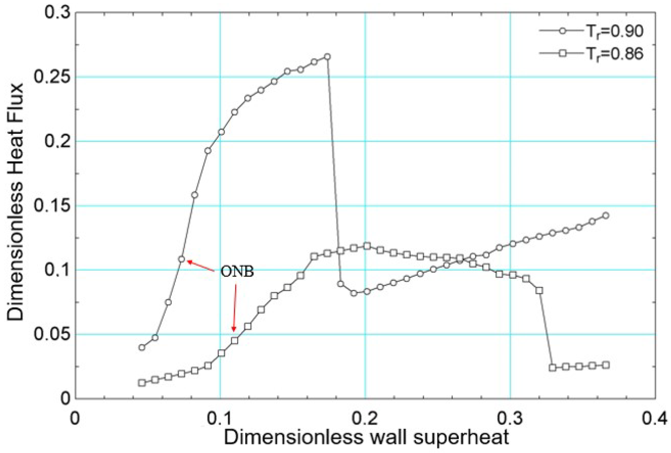
The simulations were performed with surface superheating equal to for both reduced temperatures. This value was progressively increased, considering increments of 0.001, until the final value of . The results of the average heat flux, obtained for numerical simulation for the reduced temperatures and , are presented in Figure 10. The same figure indicates the onset of nucleate boiling (ONB—onset of nucleate boiling) for both reduced temperatures. For , the onset of nucleate boiling occurs at (in lattice units), and for , it occurs at (in lattice units).
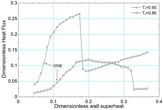
Still in relation to Figure 10, it is noted that the critical flux was higher for compared to . Considering the work of [56] and considering water as a fluid, since the works of [19,26] used the acentric factor of water, it follows that the critical flux obtained for should have been higher than that obtained for . However, it is not possible to guarantee that the parameters in lattice units for the reduced temperatures considered correspond to the simulation of the same fluid. This is justified because the transport properties were not obtained as functions of temperature despite the use of the acentric factor of water.
Regarding the critical heat flux, its strong dependence on the reduced temperature is highlighted here, as reported in the literature, for example, in [5]. Regarding the cited study, Figure 11 presents results of boiling curves for the HFE-7100 fluid at different saturation pressures considering a polished heating surface.
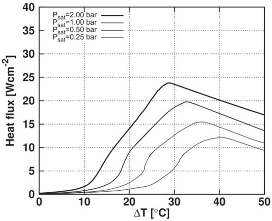
Figure 11.
Boiling curves for different saturation pressures for HFE-7100 fluid considering a polished surface.
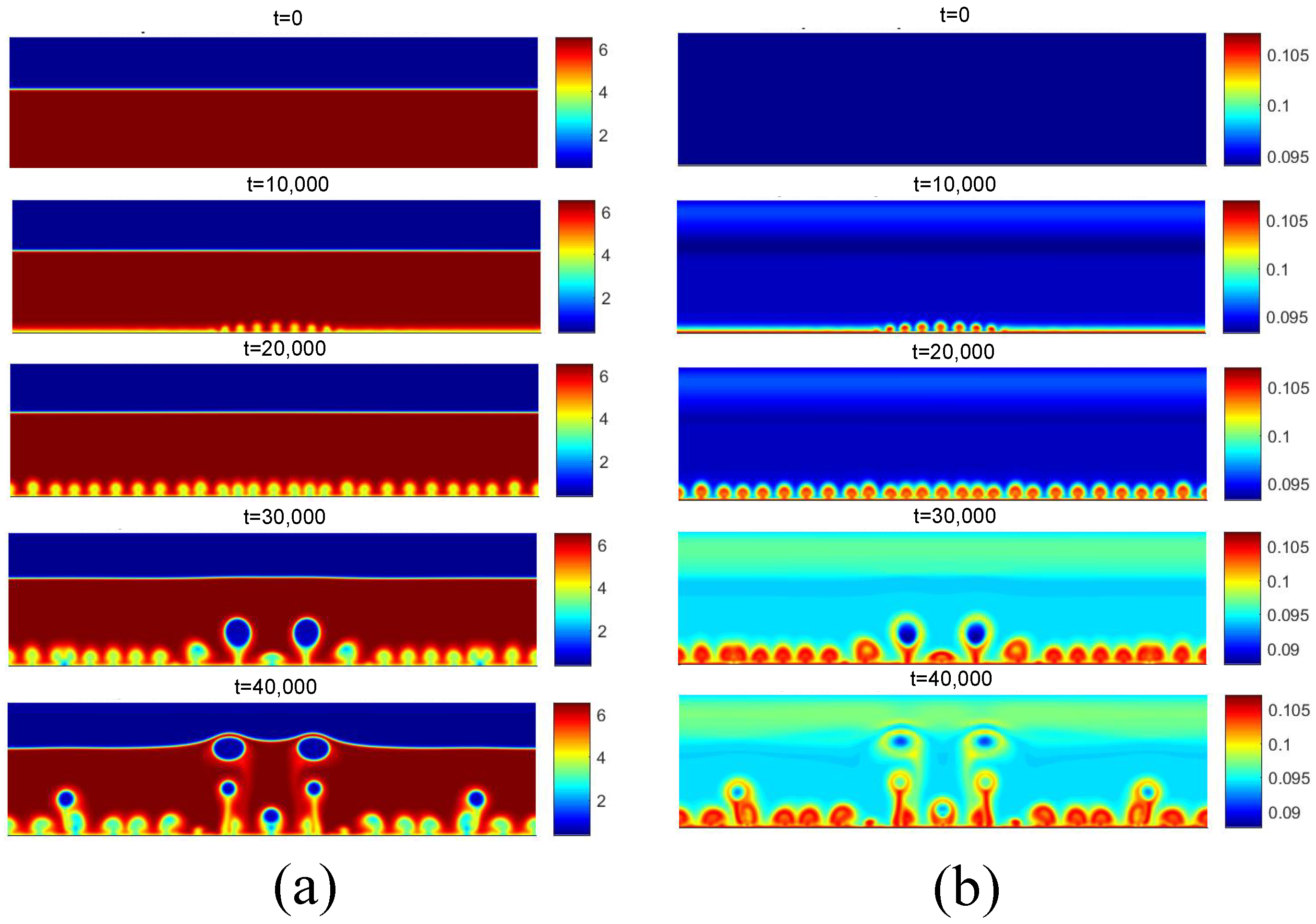
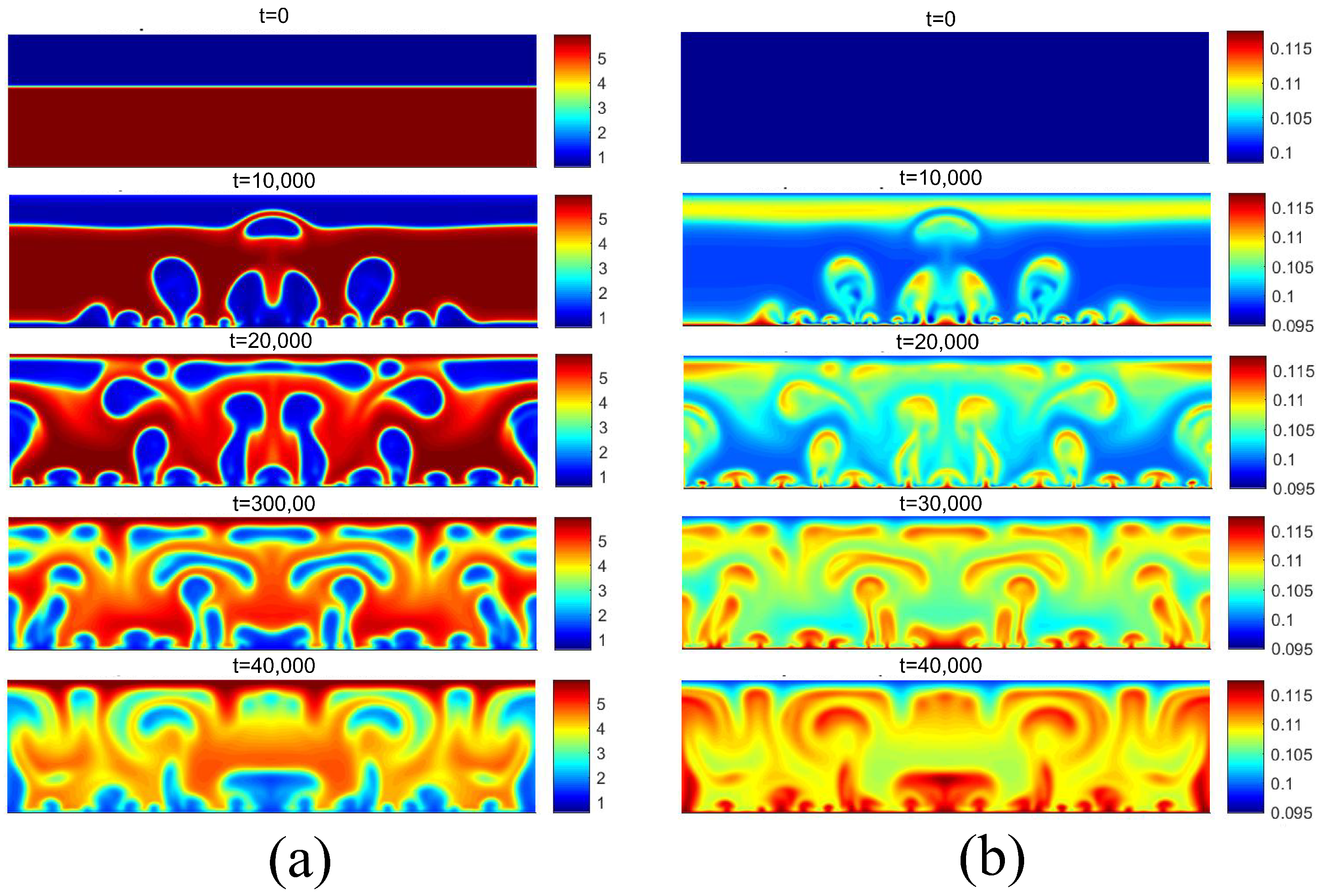
Figure 12 presents the density and temperature fields obtained for the initial boiling condition for . Regarding the density field, for t = 10,000, the reduction in density near the heated surface is observed due to the higher temperature. Subsequently, for t = 20,000, the detachment of some bubbles is observed, as well as the coalescence of nuclei in the central region. Regarding the temperature field, the effect of the increase in temperature on the liquid near the heating surface is clearly noted.
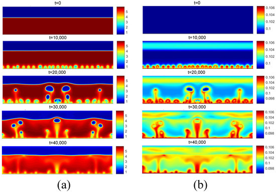
Figure 12.
(a) Density and (b) temperature fields for pool boiling for in nucleate boiling regime.
Figure 13 presents the density and temperature fields obtained for the boiling onset condition for . It can be noted that the release of the first bubbles occurs only for t = 30,000. Contrary to the results of the density field obtained for and shown in Figure 12a, no bubble coalescence is observed on the heated surface. Regarding the temperature field, the effect of increasing the temperature on the reduction in the fluid density near the heating surface can be noted.

Figure 13.
(a) Density and (b) temperature fields for pool boiling for in nucleate boiling regime.
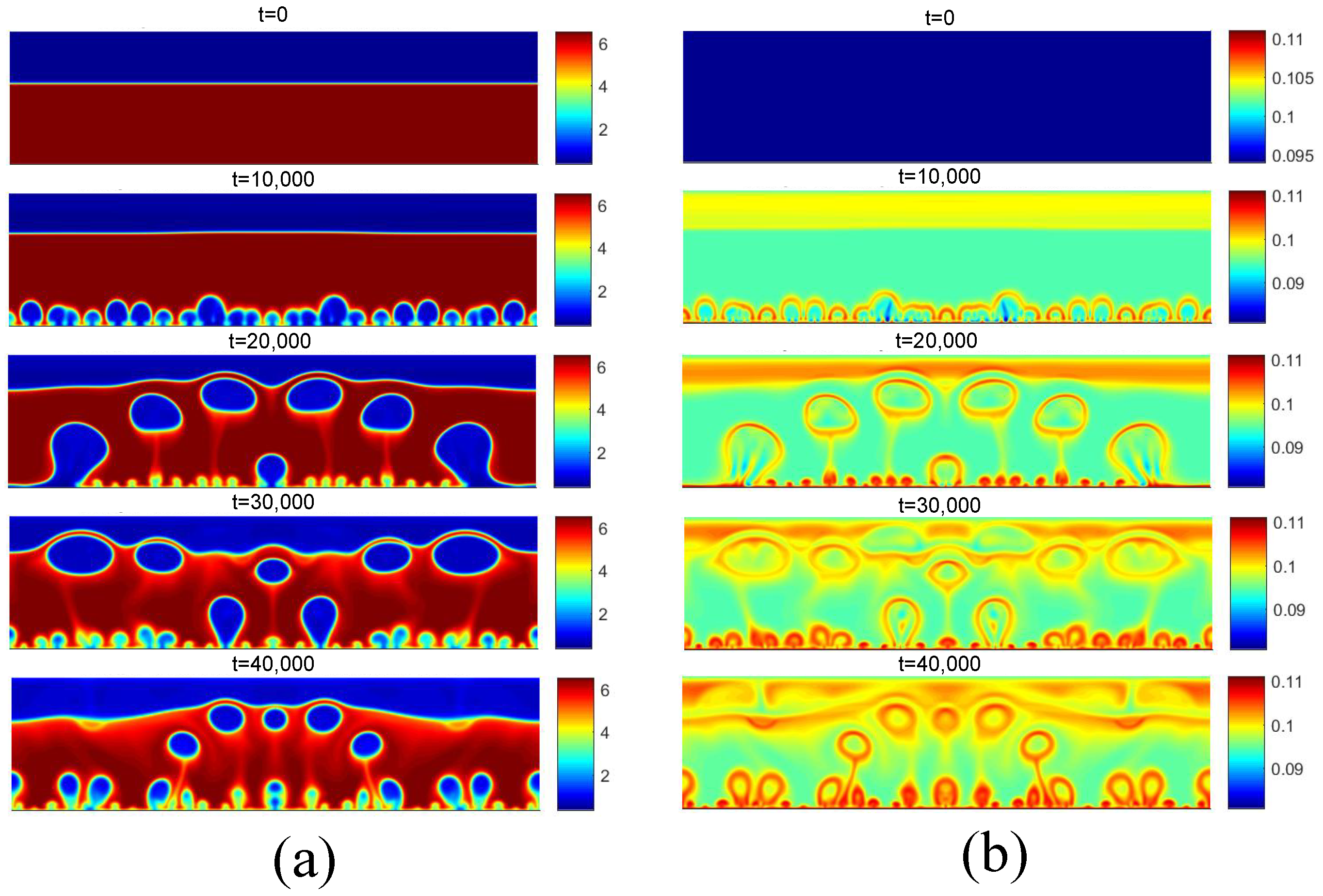
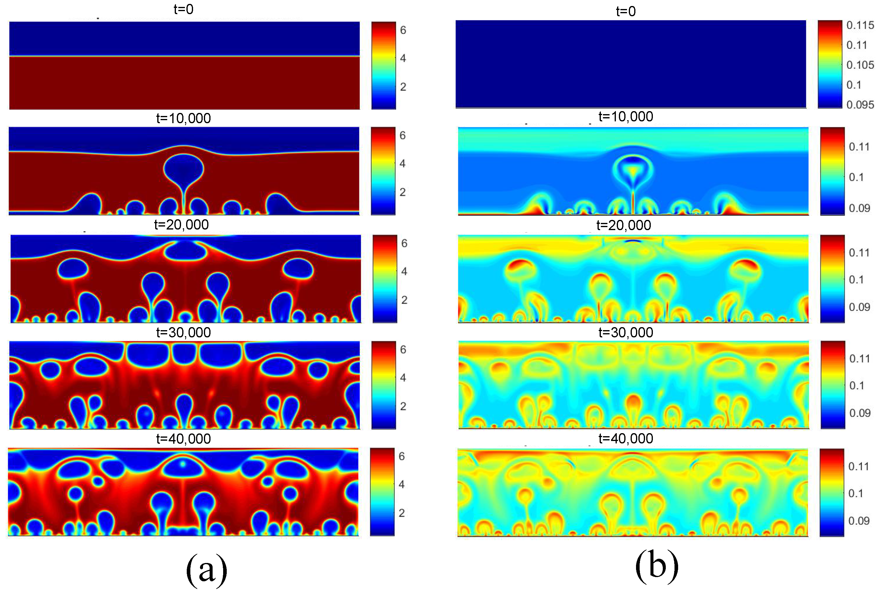
Figure 14 presents the density and temperature fields for considering . This superheating was chosen because it is located in the fully developed nucleated boiling regime. Note the presence of more vapor nuclei on the heated surface, as well as greater coalescence between bubbles, giving rise to larger bubbles.
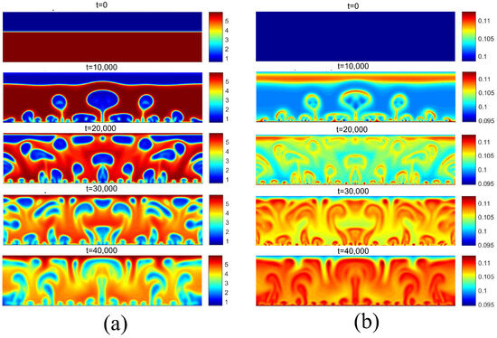
Figure 14.
(a) Density and (b) temperature fields for pool boiling for in fully developed nucleate boiling regime.
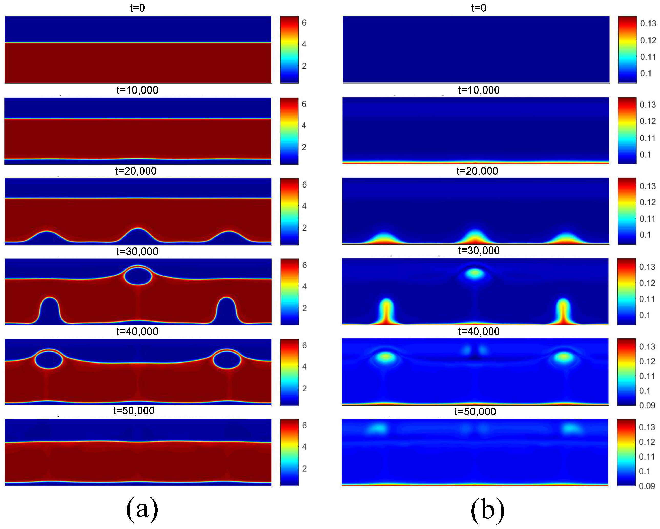
Figure 15 presents the fields for , considering the same selection criterion for the surface superheating. Again, note the presence of more vapor nuclei on the surface, as well as greater coalescence of the bubbles. Because the saturation temperature is lower, note that the bubble detachment diameter is larger than those observed for .
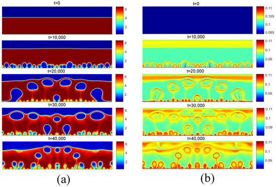
Figure 15.
(a) Density and (b) temperature fields for pool boiling for in fully developed nucleate boiling regime.
Figure 16 presents the density and temperature fields obtained for considering . For this superheat value, the critical flux condition exists, in which steam is permanently generated throughout the heating surface. An increase in superheat beyond this condition will result in the transitional boiling regime. For , the same condition is shown in Figure 17. In this case, the superheat is .

Figure 16.
(a) Density and (b) temperature fields for pool boiling for in critical flux.
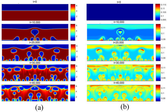
Figure 17.
(a) Density and (b) temperature fields for pool boiling for in critical flux.
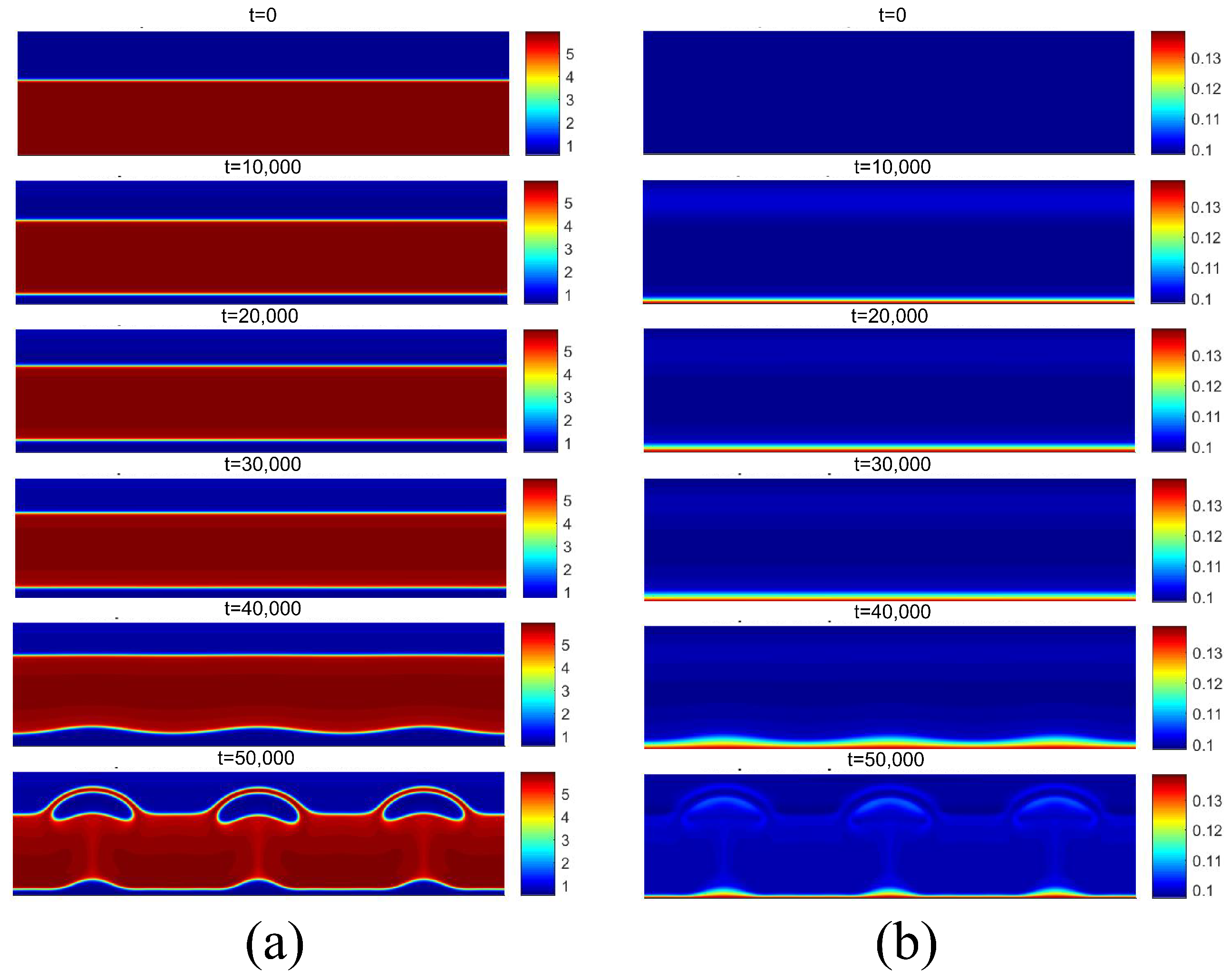
Finally, the successive increase in surface superheating beyond the critical flux condition results in the film boiling regime. For film boiling, the heat flux supplied by the heating surface is high enough to maintain a vapor film condition below the liquid. The density and temperature fields for are presented in Figure 18, and for , they are presented in Figure 19, both for the superheat condition of . Note that the heating surface is covered by a vapor film due to its high temperature. Subsequently, due to instabilities at the liquid–vapor interface, vapor bubbles are formed on the surface and detach from it.
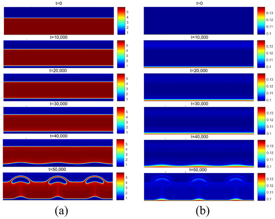
Figure 18.
(a) Density and (b) temperature fields for film boiling for .
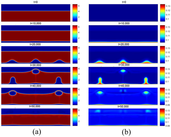
Figure 19.
(a) Density and (b) temperature fields for film boiling for .
3.2.1. Influence of Liquid Wettability
Considering the data from the work of [26], an analysis of the influence of wettability was performed using the parameter in Equation (17). The same values considered for the simulation of the bubble cycle were considered: −0.75 and 0.75. It is worth mentioning that the results of the boiling curve presented in Figure 10 for were obtained for . Thus, numerical simulations were performed only for and .
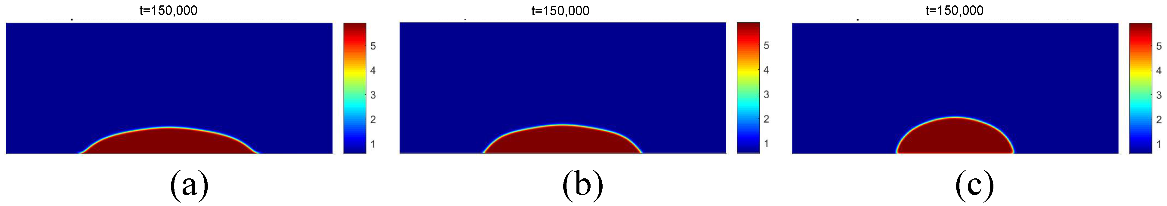
The contact angles were also obtained for the different wettability conditions. The same methodology used for the data in [20], presented previously, was used for the [26] data, except for the computational mesh: 500 × 200. The justification for the greater number of points in the X direction is due to the lower surface tension for compared to . The results of the density fields for the different contact angles are presented in Figure 20.

Figure 20.
Results of the density fields obtained for and for different values of the parameter : (a) ; (b) ; (c) .
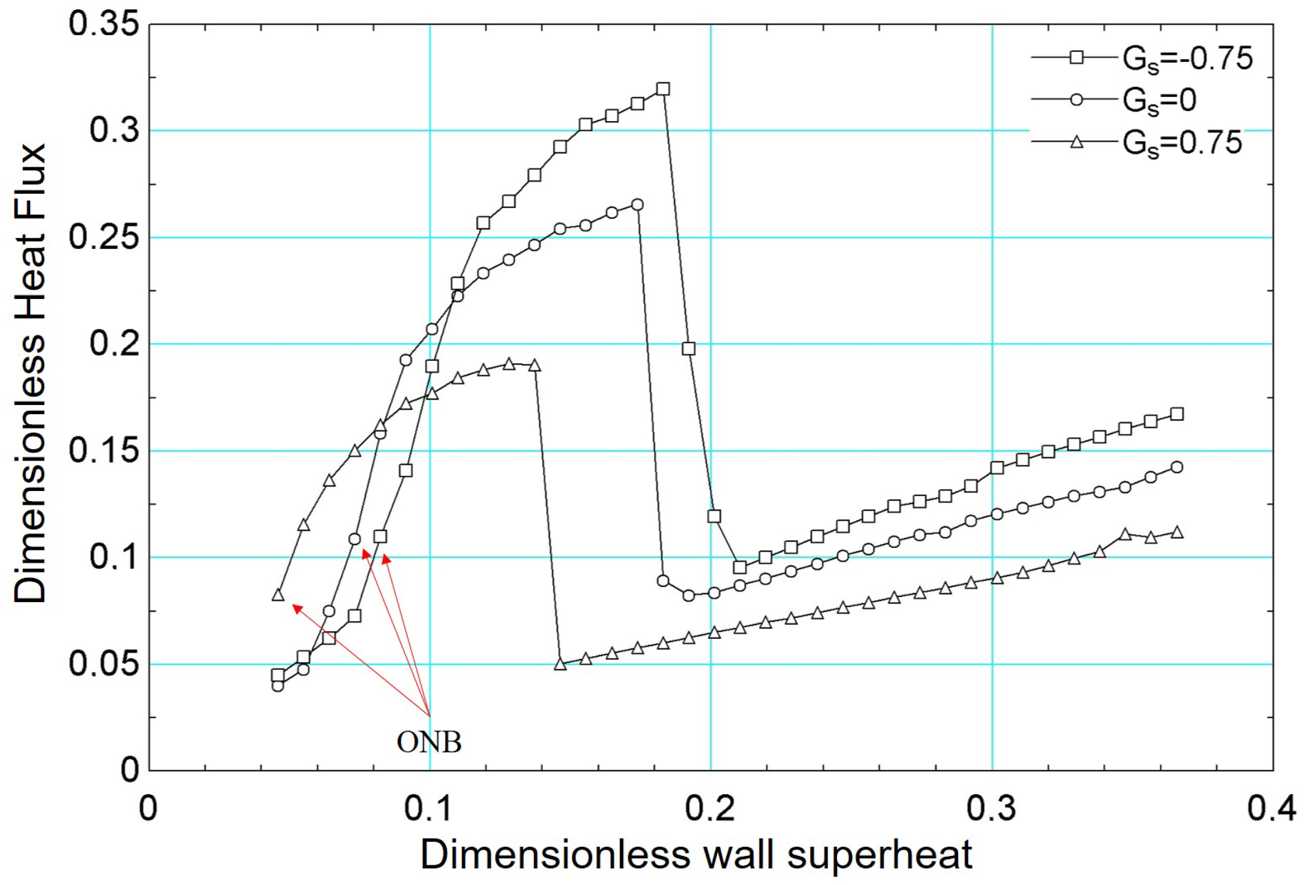
For the boiling curve simulations under varying wettability presented in Figure 21, the same fundamental methodology detailed earlier was employed. As is well established, wettability significantly influences boiling heat transfer: hydrophobic surfaces tend to exhibit larger contact angles, thus lowering the energy barrier for vapor nucleation [57] and initiating boiling at lower superheat [58]. However, they also generally display lower critical heat flux due to reduced liquid film stability near the heating surface. Conversely, hydrophilic surfaces have smaller contact angles, which delay the onset of nucleate boiling but yield higher critical heat flux. In our simulations, these trends are evident in Figure 21, where the hydrophobic surface (, °) initiates boiling at a lower superheat compared to (°) and (°), yet shows a lower peak heat flux. Conversely, surfaces with smaller contact angles (i.e., more hydrophilic) achieve progressively higher critical heat flux values, highlighting the strong interplay between contact angle, nucleation dynamics, and overall heat transfer performance.
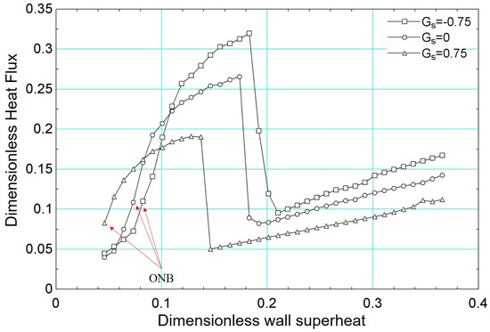
Figure 21.
Results of dimensionless heat flux versus dimensionless surface superheating for for different values of : −0.75, 0, and 0.75.
In addition, the results presented in Figure 21 can be confirmed, qualitatively, with numerical results from the literature. For example, the work published by [59] presented numerical results similar to those presented in this paper.
3.2.2. Influence of the Surface Tension
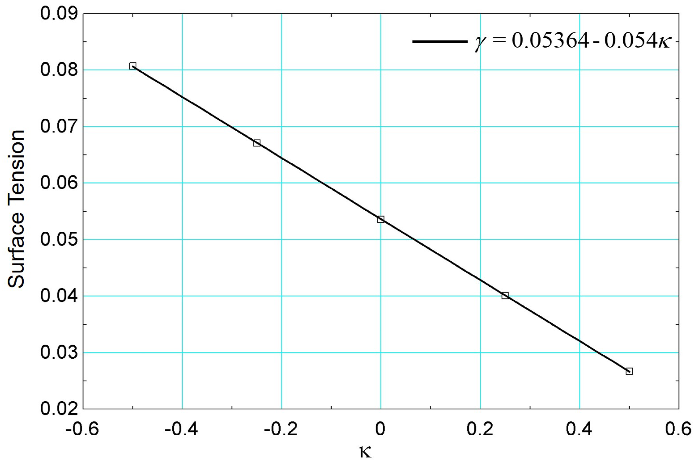
The influence of surface tension on the boiling curve results at was determined considering and . Thus, conditions of lower surface tension () and higher surface tension (), respectively, were analyzed.
Considering the same procedure performed previously through simulations of the static drop by varying the parameter , the surface tension as a function of is presented in Figure 22.
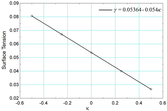
Figure 22.
Surface tension results versus parameter using data from [26].
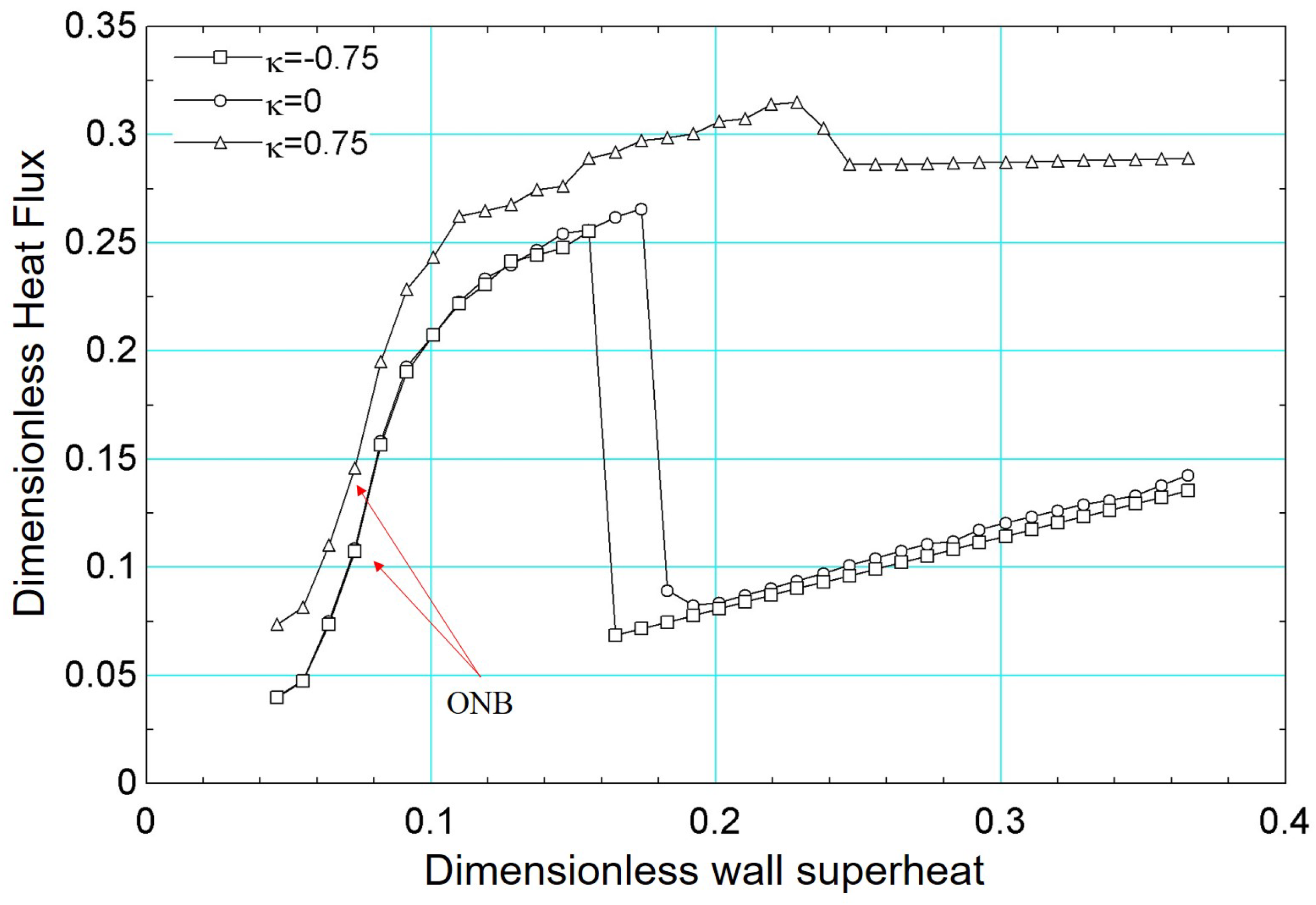
The results of the boiling curves for different values of surface tension are presented in Figure 23. It is noted that the effect of reducing the surface tension is to increase the heat flux, for the same superheat. This effect can be explained by the activation of a greater number of nucleation sites, similar to the effect caused by the addition of surfactants [60]. It is also noted that the critical flux occurs for a higher value of surface superheat. In terms of the boiling curve, it is noted that the simulation for higher surface tension () presented very similar behavior to the results of when . Note that the critical heat flux occurs for a lower value of superheat. The same is observed for the film boiling regime for and .
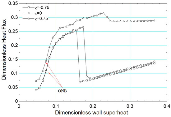
Figure 23.
Results of dimensionless heat flux versus dimensionless surface superheating for for different values of the parameter : −0.75, 0 and 0.75.
3.2.3. Influence of the Gravitational Acceleration
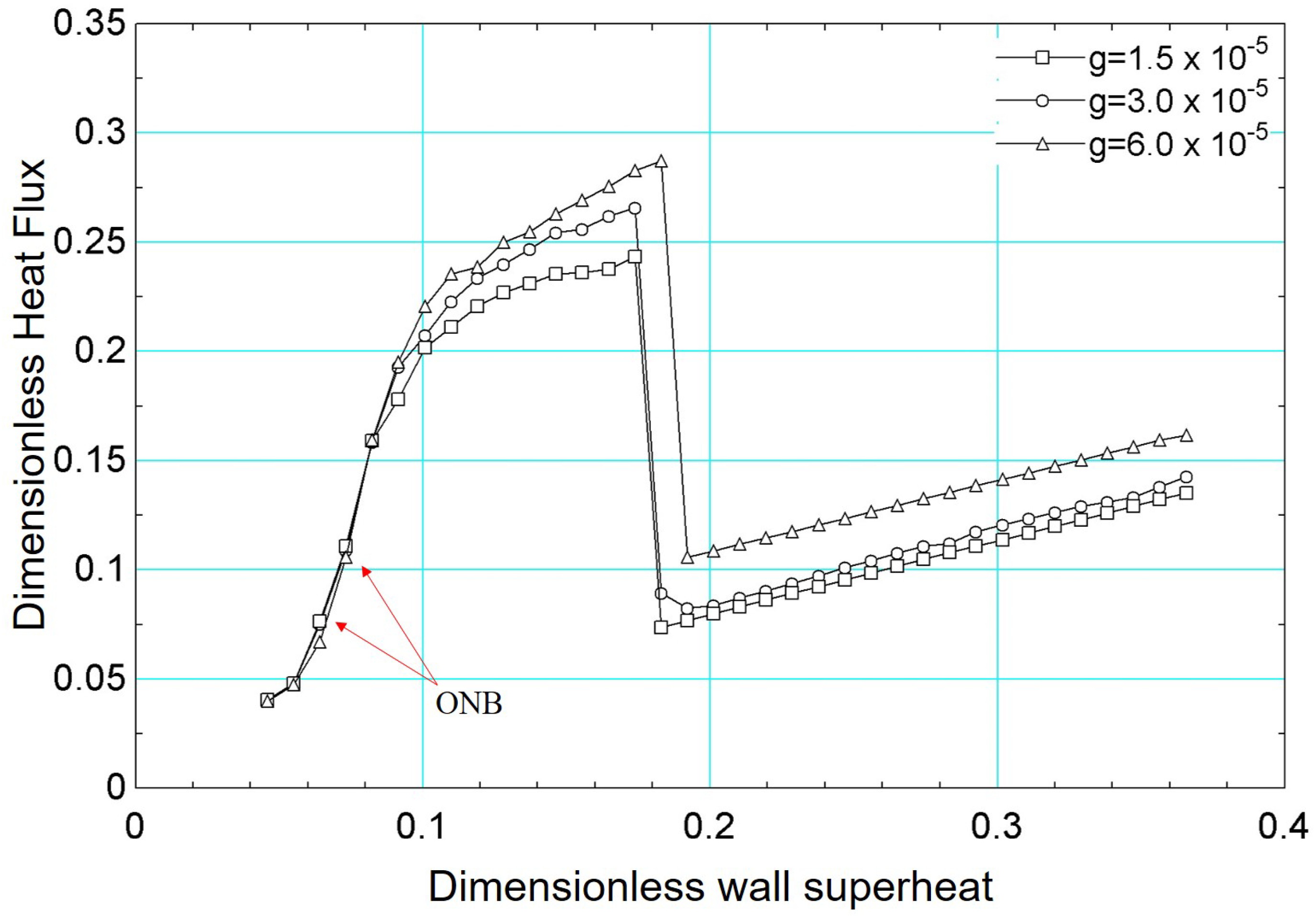
Finally, the influence of the gravitational acceleration on the boiling curve was assessed. In addition to the results obtained for , other distinct values were considered: and .
Figure 24 presents the results of the boiling curve for the gravitational acceleration values mentioned above. It is noted that the onset of boiling (onset of nucleate boiling) occurs for a lower value of surface superheating for , compared to the results obtained for the other values of gravitational acceleration.
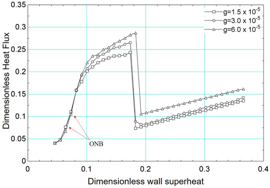
Figure 24.
Results of dimensionless heat flux versus dimensionless surface superheating for for different values of gravitational acceleration: , , .
The results in Figure 24 demonstrate that the influence of gravitational acceleration is more evident from . From this value, the effect of bubble detachment is more intense, increasing the heat flux. The critical flux is also influenced by gravitational acceleration. As shown in the figure, the critical flux is higher for and occurs for a higher superheat value. From a qualitative point of view, the numerical results presented in Figure 24 are in agreement with experimental results in the literature [61,62].
4. Conclusions
This study employed the pseudopotential lattice Boltzmann method (LBM) to investigate boiling heat transfer at different reduced temperatures, providing insights into bubble nucleation, growth, and detachment dynamics. The results demonstrated that reduced temperature significantly influences the boiling regime, affecting heat flux distribution and critical heat flux (CHF) behavior. The numerical model, based on a multi-relaxation-time approach and a Peng–Robinson equation of state, showed good agreement with theoretical predictions, validating the capability of the LBM for phase-change simulations. Additionally, this study highlighted the critical role of surface wettability in modifying boiling characteristics, where hydrophobic surfaces exhibited earlier nucleation but lower CHF, whereas hydrophilic surfaces enhanced liquid rewetting and delayed film boiling transition. Our quantitative analysis, considering contact angles spanning from approximately 36° (hydrophilic) to 63° (moderately hydrophobic), highlights two key findings. First, the onset of nucleate boiling (ONB) occurs up to 20–30% earlier for the more hydrophobic surfaces—requiring a lower superheat to initiate phase change—than it does for the hydrophilic surfaces. Second, the critical heat flux (CHF) is as much as 10–15% higher for the more hydrophilic surfaces, underscoring the benefit of smaller contact angles for sustaining robust heat transfer at higher heat fluxes. These results confirm the strong interplay between wettability and boiling performance and demonstrate the potential for tuning contact angles in order to optimize phase-change heat transfer applications. The findings emphasize the importance of accurate interface modeling and numerical stability improvements to optimize boiling heat transfer simulations. Future work could focus on refining interface tracking techniques, extending the model to three-dimensional cases, and exploring hybrid approaches to enhance computational efficiency and predictive accuracy in complex thermal systems.
Author Contributions
Conceptualization, M.d.S.G. and L.C.-G.; methodology, M.d.S.G.; software, M.d.S.G. and L.C.-G.; validation, M.d.S.G. and L.C.-G.; formal analysis, M.d.S.G. and L.C.-G.; investigation, M.d.S.G. and L.C.-G.; resources, L.C.-G.; data curation, M.d.S.G.; writing—original draft preparation, M.d.S.G.; writing—review and editing, L.C.-G.; visualization, M.d.S.G.; supervision, L.C.-G.; project administration, L.C.-G.; funding acquisition, L.C.-G. All authors have read and agreed to the published version of the manuscript.
Funding
This research received no external funding.
Data Availability Statement
The original contributions presented in this study are included in the article. Further inquiries can be directed to the corresponding author.
Acknowledgments
This study was supported, in part, by the São Paulo Research Foundation (FAPESP), Brazil, process number #2022/15765-1. The authors also acknowledge the support received from CNPq (National Council for Scientific and Technological Development, process 305771/2023-0).
Conflicts of Interest
The authors declare no conflicts of interest.
Abbreviations
The following abbreviations are used in this manuscript:
| CFD | Computational Fluid Dynamics |
| CHF | Critical Heat Flux |
| CSF | Continuum Surface Force |
| DSMC | Direct Simulation Monte Carlo |
| LBM | Lattice Boltzmann Method |
| LS | Level Set |
| MD | Molecular Dynamics |
| MRT | Multi-Relaxation Time |
| ONB | Onset of Nucleate Boiling |
| VOF | Volume of Fluid |
References
- Ishii, M.; Hibiki, T. Thermo-Fluid Dynamics of Two-Phase Flow, 2nd ed.; Springer: New York, NY, USA, 2011; pp. 1–518. [Google Scholar]
- Prosperetti, A.; Tryggvason, G. (Eds.) Computational Methods for Multiphase Flow; Cambridge University Press: Cambridge, UK, 2007; pp. 1–470. [Google Scholar]
- Carey, V.P. Liquid-Vapor Phase-Change Phenomena: An Introduction to the Thermophysics of Vaporization and Condensation Processes in Heat Transfer Equipment; CRC Press: Boca Raton, FL, USA, 2020; pp. 1–730. [Google Scholar]
- Nukiyama, S. Maximum and minimum values of heat q transmitted from metal to boiling water under atmospheric pressure. J. Soc. Mech. Eng. Jpn. 1934, 37, 367–374. [Google Scholar] [CrossRef]
- Alvariño, P.F.; Simón, M.L.S.; Guzella, M.S.; Paz, J.M.A.; Jabardo, J.M.S.; Cabezas-Gómez, L. Nucleate boiling. Experimental investigation of the CHF of HFE-7100 under pool boiling conditions on differently roughened surfaces. Int. J. Heat Mass Transf. 2019, 139, 269–279. [Google Scholar] [CrossRef]
- Sajjad, U.; Hussain, I.; Wang, C. A high-fidelity approach to correlate the nucleate pool boiling data of roughened surfaces. Int. J. Multiph. Flow 2021, 142, 103719. [Google Scholar] [CrossRef]
- Martins, I.T.; Alvariño, P.F.; Cabezas-Gómez, L. A new methodology for experimental analysis of single-cavity bubble’s nucleation, growth and detachment in saturated HFE-7100. Exp. Therm. Fluid Sci. 2024, 159, 111272. [Google Scholar]
- Ferziger, J.H.; Perić, M. Computational Methods for Fluid Dynamics; Springer: Berlin/Heidelberg, Germany, 2002; pp. 1–426. [Google Scholar]
- Tryggvason, G.; Scardovelli, R.; Zaleski, S. Direct Numerical Simulations of Gas–Liquid Multiphase Flows; Cambridge University Press: Cambridge, UK, 2011; pp. 1–324. [Google Scholar]
- Brackbill, J.U.; Kothe, D.B.; Zemach, C. Continuum Method for Modeling Surface Tension. J. Comput. Phys. 1993, 108, 175–194. [Google Scholar] [CrossRef]
- Krüger, T.; Kusumaatmaja, H.; Kuzmin, A.; Shardt, O.; Silva, G.; Viggen, E.M. The Lattice Boltzmann Method—Principles and Practice, 1st ed.; Springer: Berlin/Heidelberg, Germany, 2017; p. 694. [Google Scholar]
- Guo, Z.; Shu, C. Lattice Boltzmann Method and its Applications in Engineering, 1st ed.; World Scientific Publishing Co. Pte. Ltd.: Singapore, 2013; p. 419. [Google Scholar]
- Succi, S. The Lattice Boltzmann Equation for Fluid Dynamics and Beyond; Oxford University Press: Oxford, UK, 2001; pp. 1–308. [Google Scholar]
- Czelusniak, L.E.; Mapelli, V.P.; Guzella, M.S. Force approach for the pseudopotential lattice Boltzmann method. Phys. Rev. E 2020, 102, 033307. [Google Scholar]
- Guzella, M.S.; Czelusniak, L.E.; Mapelli, V.P.; Alvariño, P.A.; Ribatski, G.; Cabezas-Gómez, L. Simulation of Boiling Heat Transfer at Different Reduced Temperatures with an Improved Pseudopotential Lattice Boltzmann Method. Symmetry 2020, 12, 1358. [Google Scholar] [CrossRef]
- Jaramillo, A.; Mapelli, V.P.; Cabezas-Gómez, L. Pseudopotential Lattice Boltzmann Method for boiling heat transfer: A mesh refinement procedure. Appl. Therm. Eng. 2022, 213, 118705. [Google Scholar]
- Shan, X.; Chen, H. Lattice Boltzmann model for simulating flows with multiple phases and components. Phys. Rev. E 1993, 47, 1815–1820. [Google Scholar]
- Shan, X.; Chen, H. Simulation of nonideal gases and liquid-gas phase transitions by the lattice Boltzmann equation. Phys. Rev. E 1994, 49, 2941–2948. [Google Scholar]
- Li, Q.; Kang, Q.J.; Francois, M.M.; He, Y.L.; Luo, K.H. Lattice Boltzmann modeling of boiling heat transfer: The boiling curve and the effects of wettability model: Methods and applications. Int. J. Heat Mass Transf. 2015, 85, 787–796. [Google Scholar] [CrossRef]
- Li, Q.; Zhou, P.; Yan, H.J. Improved thermal lattice Boltzmann model for simulation of liquid-vapor phase change. Phys. Rev. E 2017, 96, 063303. [Google Scholar] [CrossRef] [PubMed]
- Huang, H.B.; Krafczyk, M.; Lu, X. Forcing term in single-phase and Shan-Chen-type multiphase lattice Boltzmann models. Phys. Rev. E 2011, 84, 046710. [Google Scholar] [CrossRef]
- Shan, X. Analysis and reduction of the spurious current in a class of multiphase lattice Boltzmann models. Phys. Rev. E 2006, 73, 047701. [Google Scholar] [CrossRef]
- Shan, X. Pressure tensor calculation in a class of nonideal gas lattice Boltzmann models. Phys. Rev. E 2008, 77, 066702. [Google Scholar] [CrossRef] [PubMed]
- Li, Q.; Luo, K.H.; Kang, Q.J.; Chen, Q.; Liu, Q. Lattice Boltzmann methods for multiphase flow and phase-change heat transfer. Prog. Energy Combust. Sci. 2016, 9, 62–105. [Google Scholar] [CrossRef]
- Mu, Y.T.; Chen, L.; He, Y.L.; Kang, Q.J.; Tao, W.Q. Nucleate boiling performance evaluation of cavities at mesoscale level. J. Heat Mass Transf. 2017, 106, 708–719. [Google Scholar] [CrossRef]
- Gong, S.; Cheng, P. Nucleate boiling. Direct numerical simulations of pool boiling curves including heater’s thermal responses and the effect of vapor phase’s thermal conductivity. Int. Commun. Heat Mass Transf. 1963, 87, 61–71. [Google Scholar] [CrossRef]
- Fogliatto, E.O.; Clausse, A.; Teruel, F.E. Evelopment of a double-mrt pseudopotential model for tridimensional boiling simulation. Int. J. Therm. Sci. 2022, 179, 107637. [Google Scholar] [CrossRef]
- Liang, H.; Liu, W.; Li, Y.; Wei, Y. A thermal lattice Boltzmann model for evaporating multiphase flows. Phys. Fluids 2024, 36, 032101. [Google Scholar] [CrossRef]
- Zhang, C.; Chen, L.; Ji, W.; Liu, Y.; Liu, L.; Tao, W.Q. Lattice boltzmann mesoscopic modeling of flow boiling heat transfer processes in a microchannel. Appl. Therm. Eng. 2021, 197, 117369. [Google Scholar] [CrossRef]
- Song, Y.; Mu, X.; Wang, J.; Shen, S.; Liang, G. Channel flow boiling on hybrid wettability surface with lattice boltzmann method. Appl. Therm. Eng. 2021, 233, 121191. [Google Scholar]
- Li, J.; Le, D.V.; Li, H.; Zhang, X.; Kang, C.W.; Lou, J. Hybrid outflow boundary condition for the pseudopotential lbm simulation of flow boiling. Int. J. Therm. Sci. 2024, 196, 108741. [Google Scholar]
- Sayyari, M.J.; Ahmadian, M.H.; Kim, K.C. Three-dimensional condensation in a vertical channel filled with metal foam using a pseudopotential lattice boltzmann model. Int. J. Therm. Sci. 2024, 172, 107352. [Google Scholar]
- Peng, H.; Zhang, J.; He, X.; Wang, Y. Thermal pseudo-potential lattice boltzmann method for simulating cavitation bubbles collapse near a rigid boundary. Comput. Fluids 2024, 217, 104817. [Google Scholar]
- Zhang, R.; Chen, H. Lattice Boltzmann method for simulations of liquid-vapor thermal flows. Phys. Rev. E 2003, 67, 066711. [Google Scholar]
- Hazi, G.; Markus, A. On the bubble departure diameter and release frequency based on numerical simulation results. Int. J. Heat Mass Transf. 2009, 52, 1472–1480. [Google Scholar]
- Gong, S.; Cheng, P. A lattice Boltzmann method for simulation of liquid-vapor phase-change heat transfer. Int. J. Heat Mass Transf. 2012, 55, 4923–4927. [Google Scholar] [CrossRef]
- Gong, S.; Cheng, P. Lattice Boltzmann simulations for surface wettability effects in saturated pool boiling heat transfer. Int. J. Heat Mass Transf. 2015, 85, 635–646. [Google Scholar]
- Gong, S.; Cheng, P. Numerical simulation of pool boiling heat transfer on smooth surfaces with mixed wettability by lattice Boltzmann method. Int. J. Heat Mass Transf. 2015, 80, 206–216. [Google Scholar]
- Taleghani, A.S.; Noori, M.S. Numerical investigation of coalescence phenomena, affected by surface acoustic waves. Eur. Phys. J. Plus 2022, 137, 975. [Google Scholar]
- Noori, M.S.; Taleghani, A.S. Numerical investigation of two-phase flow control based on the coalescence under variation of gravity conditions. Eur. Phys. J. Plus 2024, 139, 1–13. [Google Scholar]
- Schukmann, A.; Hass, V.; Schneider, A. Spurious Aeroacoustic Emissions in Lattice Boltzmann Simulations on Non-Uniform Grids. Fluids 2025, 10, 31. [Google Scholar] [CrossRef]
- Li, Q.; Luo, K.H.; Li, X.J. Lattice Boltzmann modeling of multiphase flows at large density ration with an improved pseudopotential model. Phys. Rev. E 2013, 87, 053301. [Google Scholar]
- Li, Q.; Luo, K.H. Achieving tunable surface tension in the pseudopotential lattice Boltzmann modeling of multiphase flows. Phys. Rev. E 2013, 88, 053307. [Google Scholar]
- Lallem, P.; Luo, L. Theory of the lattice Boltzmann method: Dispersion, dissipation, isotropy, Galilean invariance, and stability. Phys. Rev. E 2000, 61, 6546. [Google Scholar]
- Yuan, P.; Schaefer, L. Equations of state in a lattice Boltzmann model. Phys. Fluids 2006, 18, 101–112. [Google Scholar]
- Chen, L.; Kang, Q.; Mu, Y.; He, Y.; Tao, W. A critical review of the pseudopotential multiphase lattice Boltzmann model: Methods and applications. Int. J. Heat Mass Transf. 2014, 76, 210–236. [Google Scholar] [CrossRef]
- Lee, T.; Lin, C. A stable discretization of the lattice Boltzmann equation for simulation of incompressible two-phase flows at high density ratio. J. Comput. Phys. 2005, 1, 16–47. [Google Scholar]
- Ginzbourg, I.; Adler, P. Boundary flow condition analysis for the three-dimensional lattice Boltzmann model. J. Phys. II 1994, 4, 191–214. [Google Scholar]
- Zou, Q.; He, X. On pressure and velocity boundary conditions for the lattice Boltzmann BGK model. Phys. Fluids 1997, 9, 1591–1598. [Google Scholar]
- Caiazzo, A. Analysis of lattice Boltzmann initialization routines. J. Stat. Phys. 2005, 121, 37–48. [Google Scholar]
- Mei, R.; Luo, L.; Lallem, P.; d’Humieres, D. Consistent initial conditions for lattice Boltzmann simulations. J. Stat. Phys. 2006, 35, 855–862. [Google Scholar]
- Gong, S.; Cheng, P. Lattice Boltzmann simulation of periodic bubble nucleation, growth and departure from a heated surface in pool boiling. Int. Heat Mass Transf. 2013, 64, 122–132. [Google Scholar]
- Son, G.; Dhir, V.K. Dynamics and Heat Transfer Associated with a Single Bubble During Nucleate Boiling on a Horizontal Surface. J. Heat Transf. 1999, 64, 623–631. [Google Scholar] [CrossRef]
- Fritz, W. Maximum volume of vapour bubbles. Phys. Zeitschr 1935, 36, 379–384. [Google Scholar]
- Zuber, N. Nucleate boiling. The region of isolated bubbles and the similarity with natural convection. Int. J. Heat Mass Transf. 1963, 6, 53–78. [Google Scholar] [CrossRef]
- Zuber, N. Nucleate boiling. On the stability of boiling heat transfer. Trans. ASME 1958, 80, 711–720. [Google Scholar]
- Kim, S.H.; Lee, G.C.; Kang, J.Y.; Moriyama, K.; Park, H.S.; Kim, M.H. The role of surface energy in heterogeneous bubble growth on ideal surface. Int. J. Heat Mass Transf. 2017, 108, 1901–1909. [Google Scholar] [CrossRef]
- Bourdon, B.; Bertr, E.; Di Marco, P.; Marengo, M.; Rioboo, R.; De Coninck, J. Wettability influence on the onset temperature of pool boiling: Experimental evidence onto ultra-smooth surfaces. Adv. Colloid Interface Sci. 2015, 221, 34–40. [Google Scholar]
- Hsu, H.; Lin, M.; Popovic, B.; Lin, C.; Patankar, N.A. A numerical investigation of the effect of surface wettability on the boiling curve. PLoS ONE 2017, 12, 0187175. [Google Scholar] [CrossRef] [PubMed]
- Elghanam, R.I.; Fawal, M.M.E.L.; Aziz, R.A.; Skr, M.H.; Khalifa, A.H. Experimental study of nucleate boiling heat transfer enhancement by using surfactant. Ain Shams Eng. J. 2011, 2, 195–209. [Google Scholar]
- Raj, R.; Kim, J.; McQuillen, J. Gravity Scaling Parameter for Pool Boiling Heat Transfer. J. Heat Transf. 2010, 132, 091502. [Google Scholar]
- Colin, C.; Kannengieser, O.; Bergez, W.; Lebon, M.; Sebilleau, J.; Sagan, M.; Tanguy, S. Nucleate pool boiling in microgravity: Recent progress and future prospects. Comptes Rendus Mec. 2017, 345, 21–34. [Google Scholar]


Disclaimer/Publisher’s Note: The statements, opinions and data contained in all publications are solely those of the individual author(s) and contributor(s) and not of MDPI and/or the editor(s). MDPI and/or the editor(s) disclaim responsibility for any injury to people or property resulting from any ideas, methods, instructions or products referred to in the content. |
© 2025 by the authors. Licensee MDPI, Basel, Switzerland. This article is an open access article distributed under the terms and conditions of the Creative Commons Attribution (CC BY) license (https://creativecommons.org/licenses/by/4.0/).