Tabulated Chemistry Models for Numerical Simulation of Combustion Flow Field

Abstract

In numerical simulations of combustion flow fields, tabulated chemistry models are widely used to reduce computational cost compared to rigorous reaction calculation methods such as detailed chemical reaction calculations. Tabulated combustion data are generated by performing low-dimensional combustion calculations prior to simulating the combustion flow field. The results are then stored in a database indexed by parameters such as mixture fraction and reaction progress variables. In recent years, significant advancements have been made in the tabulation of combustion data to accommodate diverse fuels and replicate the complex conditions observed in practical combustion systems. This review paper provides an overview of recent developments in tabulated chemistry models, particularly those based on the flamelet/progress-variable method. It specifically addresses scenarios involving multi-point fuel injection, the presence of heat loss factors in combustion flow fields, the consideration of varying diffusion coefficients, and other complex phenomena.

1. Introduction

In numerical simulations of combustion flow fields, detailed chemical reaction calculations are generally considered the most accurate method for predicting chemical reactions in combustion. However, to reduce the computational cost associated with such calculations, alternative approaches, such as multi-step global reaction models or methods that utilize tabulated chemical reaction data, are widely adopted. This review summarizes recent advancements and trends in the use of tabulated chemical reaction data.

In the analysis of actual combustion fields, the combustion characteristics of various flame types are often classified using the flame index (F.I.), which serves as a diagnostic tool for investigating flame structures [1]. The F.I. has been applied to the analysis of several flame types in recent studies (e.g., [2]). The flame index is defined as the scalar product of the spatial gradients of the fuel and oxidizer mass fractions, expressed as follows:

$$\begin{array}{c}\hfill \mathrm{F}.\mathrm{I}.=\nabla Y_f·\nabla Y_{{\mathrm{O}}_2},\end{array}$$

(1)

where $Y_f$ and $Y_{{\mathrm{O}}_2}$ denote the mass fractions of the fuel and oxidizer, respectively. The calculated F.I. can be used to distinguish between premixed flames and diffusion flames, with positive values indicating premixed flames and negative values indicating diffusion flames.

Figure 1 illustrates an example of simultaneous premixed and diffusion combustion, as demonstrated by the instantaneous F.I. distribution along the central cross-section of a coal-jet flame [2,3]. Here, $Y_f=Y_{{\mathrm{C}}_a{\mathrm{H}}_b{\mathrm{O}}_c}+Y_{\mathrm{CO}}$, where ${\mathrm{C}}_a{\mathrm{H}}_b{\mathrm{O}}_c$ represents the volatile matter devolatized from heated coal particles. This formulation is commonly used in coal combustion simulations. The image reveals three distinct flame layers—diffusion (F.I. < 0), premixed (F.I. > 0), and diffusion (F.I. < 0)—arranged from the inner to the outer regions of the flame. The reactions in each layer can be analyzed by examining the spanwise profiles of the instantaneous mass fractions of ${\mathrm{C}}_a{\mathrm{H}}_b{\mathrm{O}}_c$, O₂, CO₂, and CO, as well as the chemical reaction rates of ${\mathrm{C}}_a{\mathrm{H}}_b{\mathrm{O}}_c$ and $\mathrm{CO}$. In the middle of the streamwise direction, both ${\mathrm{C}}_a{\mathrm{H}}_b{\mathrm{O}}_c$ and ${\mathrm{O}}_2$ decrease radially, with their reaction rates peaking in the second inner layer, indicating a premixed flame. Additionally, $\mathrm{CO}$ and ${\mathrm{O}}_2$ decrease radially in the outermost layer, with reaction rate peaks observed, signifying a diffusion flame. These characteristics suggest that the reactions of volatile matter with O₂ in the coal-carrier air occur in the inner premixed flame layer, while the reactions of volatile matter with CO and O₂ in the surrounding air take place in the outer diffusion flame layer. The negative F.I. values in the innermost layer can be explained by the instantaneous distributions of the normalized devolatilization rates for individual particles, represented by particle color. A significant release of volatile matter is observed in this innermost layer, indicating the formation of a diffusion layer where F.I. is <0. Although regions with a low ${\mathrm{O}}_2$ consumption rate are not present, the rate of volatile matter production via devolatilization exceeds the rate of volatile matter consumption during premixed combustion. As a result, $Y_{{\mathrm{C}}_a{\mathrm{H}}_b{\mathrm{O}}_c}$ increases radially, leading to negative F.I. values.

Flamelet models, which compile laminar flame characteristics into a tabulated database such as the flamelet-generated manifold (FGM) [4,5] method and the flamelet/progress-variable (FPV) [6] method are widely used for premixed and diffusion combustion, respectively. The process of tabulating chemical reaction data differs between diffusion combustion and premixed combustion. In the FPV method, one-dimensional counterflow diffusion flames are simulated using a detailed chemical reaction mechanism, and a database of temperature and species concentrations is generated with respect to the mixture fraction and progress variable. Since one-dimensional counterflow diffusion flames are employed, the resulting database inherently reflects the characteristics of diffusion combustion. In simulations of actual combustion flow fields, the conservation equations for the mixture fraction and progress variable are solved to determine temperature and species concentrations. In contrast, the flamelet–generated manifold (FGM) method involves solving one-dimensional laminar premixed flame propagation using a detailed chemical reaction mechanism for premixed, unburned gases at various equivalence ratios. This process generates a database of temperature and species concentrations indexed by equivalence ratio and progress variable. By converting the equivalence ratio to the mixture fraction, a database comparable to that used in the FPV method can be obtained. Since one-dimensional laminar premixed flame propagation is utilized, the resulting database inherently reflects the characteristics of premixed combustion.

In the FPV approach, a tabulated chemical reaction database, or flamelet library, is typically generated by solving the following flamelet equation under the assumption of a unity Lewis number:

$$\begin{array}{c}\hfill \rho {\displaystyle \frac{\partial Y_k}{\partial t}}-{\displaystyle \frac{\rho \chi }{2}}{\displaystyle \frac{{\partial }^2{Y}_k}{\partial Z^2}}-{\dot{\omega }}_k=0\end{array}$$

(2)

$$\begin{array}{c}\hfill \begin{array}{c}\hfill \rho {\displaystyle \frac{\partial T}{\partial t}}-{\displaystyle \frac{\rho \chi }{2}}\left({\displaystyle \frac{{\partial }^{2}T}{\partial Z^2}}+{\displaystyle \frac{1}{c_p}}{\displaystyle \frac{\partial c_p}{\partial Z}}{\displaystyle \frac{\partial T}{\partial Z}}\right)+{\displaystyle \sum _k}{\displaystyle \frac{\rho \chi }{2}}\left({\displaystyle \frac{\partial Y_k}{\partial Z}}+{\displaystyle \frac{Y_k}{W}}{\displaystyle \frac{\partial W}{\partial Z}}\right)\\ \hfill \times \left(1-{\displaystyle \frac{c_{pk}}{c_p}}\right){\displaystyle \frac{\partial T}{\partial Z}}+{\displaystyle \frac{1}{c_p}}{\displaystyle \sum _k}{h}_k{\dot{\omega }}_k=0\end{array}\end{array}$$

(3)

where $\rho$, $Y_k$, and ${\dot{\omega }}_k$ represent the density and mass fraction of species k and its source term, respectively. $\chi$ is the scalar dissipation rate, T is the temperature, $c_p$ is the specific heat capacity at constant pressure, $c_{pk}$ is the specific heat capacity of species k at constant pressure, and W is the mean molecular weight of the mixture. For example, these equations are solved using tools such as Flamemaster [7].

Figure 2 provides an example of a tabulated chemical reaction database, or flamelet library, illustrating the distribution of the mass fraction of OH ($Y_{\mathrm{OH}}$) as a function of the mixture fraction (Z) and progress variable (C). The database includes the mass fraction of chemical species ($Y_k$), the reaction rate (${\dot{\omega }}_k$), and the enthalpy ($h_k$) for each chemical species (k) present in the combustion flow field. In a numerical simulation of a combustion flow field, the conservation equations for Z and C are solved. Using Z and C as indices, the database is referenced to obtain the distribution of physical quantities within the combustion flow field. When using Reynolds-averaged Navier-Stokes (RANS) simulations or Large-eddy simulations (LES) for flow analysis in a combustion field, a method called the Flamelet Revised for consistencies (FlaRe) approach has been proposed. This approach appropriately accounts for the subgrid-scale variance of the progress variable (C) in relation to the scalar dissipation rate [8,9,10,11]. The FlaRe approach has been extensively tested using RANS and LES for premixed and partially premixed combustion fields; these studies are reviewed in [12].

2. Applicability to Various Fuels

Flamelet methods have been applied to a wide range of turbulent combustion problems, from laboratory-scale burners (e.g., [13,14,15]) to flames inside combustors (e.g., [16,17]), and furnaces [18,19]. A fundamental study on the Flamelet/Progress-Variable Approach (FPVA) for spray flames was conducted by Baba and Kurose [20], while a study on coal flames was conducted by Watanabe and Yamamoto [21]. Figure 3 provides an overview of the data interaction between physical space and mixture fraction (Z) space. In Figure 3, FPVA-P and FRVA-E define the progress variable (C) as the combustion products ($C=Y_{{\mathrm{CO}}_2}+Y_{{\mathrm{H}}_2\mathrm{O}}$) and the total enthalpy of chemical species, respectively. In the FPV method, the conservation equations for the mixture fraction (Z) and progress variable (C) are solved in physical space, and the temperature (T), mass fraction of chemical species ($Y_k$), and reaction rates(${\dot{\omega }}_k$) are obtained by referencing a database or Chemtable using Z and C as indices. The Steady Flamelet Model (SFM) shown in the figure refers to the classical flamelet method proposed by Peters [22], which does not take into account the progress variable.

Figure 4 presents an analysis of the spray flame using FPV methods [20]. Figure 4B compares the calculation results for each condition using the Liquid Fuel Arrhenius formulation (LAR), Liquid Fuel Steady-Flamelet Model (LFM), Liquid Fuel Modified Steady-Flamelet Model (LFMM), and Liquid Fuel Flamelet/Progress-Variable models (LFM-P and LFM-E). As shown in Figure 4B, the results obtained using the FPV method (Figure 4B(d,e)) closely reproduce the exact solution derived from the Arrhenius method (Figure 4B(a)). In particular, Figure 4B(e), which uses enthalpy (h) as the progress variable, demonstrates significantly better performance compared to the other cases. This improvement is attributed to the inclusion of the effects of enthalpy increases caused by the high-temperature coflow and the mass transfer from droplets to the gaseous phase through evaporation. However, it should be noted that the enthalpy in the flamelet library does not account for the increases caused by high-temperature coflow in flame stabilization or the mass transfer resulting from droplet evaporation in the flow field.

Figure 5 illustrates an analysis of piloted pulverized coal/ammonia co-combustion using FPV methods [23]. In this investigation, turbulent mixing occurs among four fuel streams: volatile matter, char off-gases, pilot fuel, and the ammonia. For such multi-fuel streams, the mixing process is described using multiple mixture fractions, defined as follows:

$$\begin{array}{c}\hfill Z_{vol}={\displaystyle \frac{{\xi }_{vol}}{{\xi }_{vol}+{\xi }_{pro}+{\xi }_{pil}+{\xi }_{am}+{\xi }_{ox}}},\end{array}$$

(4)

$$\begin{array}{c}\hfill Z_{pro}={\displaystyle \frac{{\xi }_{pro}}{{\xi }_{vol}+{\xi }_{pro}+{\xi }_{pil}+{\xi }_{am}+{\xi }_{ox}}},\end{array}$$

(5)

$$\begin{array}{c}\hfill Z_{pil}={\displaystyle \frac{{\xi }_{pil}}{{\xi }_{vol}+{\xi }_{pro}+{\xi }_{pil}+{\xi }_{am}+{\xi }_{ox}}},\end{array}$$

(6)

$$\begin{array}{c}\hfill Z_{am}={\displaystyle \frac{{\xi }_{am}}{{\xi }_{vol}+{\xi }_{pro}+{\xi }_{pil}+{\xi }_{am}+{\xi }_{ox}}},\end{array}$$

(7)

where $Z_{vol}$, $Z_{pro}$, $Z_{pil}$, and $Z_{am}$ represent the mixture fractions of gas originating from the volatile matter, char off-gases, pilot fuel, and ammonia, respectively. Similarly, ${\xi }_{vol}$, ${\xi }_{pro}$, ${\xi }_{pil}$, ${\xi }_{am}$, and ${\xi }_{ox}$ denote the mass of gas originating from the volatile matter, char off-gases, pilot fuel, ammonia, and the oxidizer in the local computational cell, respectively [23]. In this study, the NOx formation mechanism in the coal/ammonia co-firing flame was investigated and thoroughly evaluated through conditional reaction pathway analyses. However, as the number of mixture fractions increases [24,25], the dimension of the flamelet database grows, leading to an inevitable expansion of database size. The next chapter discusses strategies to address the challenges posed by this increasing database size.

3. Consideration of Flow and Chemical Properties

3.1. Effect of Adiabaticity in the Flow Field

Modern combustors, such as gas turbines and boilers, are subject to significant heat losses through the combustor walls. A local decrease in the combustion flow-field temperature due to heat loss can alter the chemical equilibrium and affect the mass fractions of chemical species. In such scenarios, heat loss can be incorporated into the flamelet library using the approach proposed by Proch and Kempf [26], which involves scaling the source term in the energy equation of the flamelet equation (Equation (3)) by adding a term as follows:

$$-{\displaystyle \frac{\alpha }{c_p}}\sum _k{h}_k{\dot{\omega }}_k,$$

(8)

where $\alpha$ is the correction factor representing heat loss. However, estimating the magnitude of this heat loss requires solving of the enthalpy transport equation during the simulation of the heat flow field [27,28].

Figure 6 shows a study of ${\mathrm{H}}_2/{\mathrm{O}}_2$ combustion in a coaxial combustor [29,30] using the previously mentioned FPV method, which accounts for heat loss (non-adiabatic FPV, NA-FPV) [27]. Figure 6b compares the streamwise profile of the time-averaged wall heat flux predicted by the FPV and NA-FPV approaches with the measured data. The results clearly demonstrate that the NA-FPV approach outperforms the FPV approach in predicting wall heat flux across the entire region.

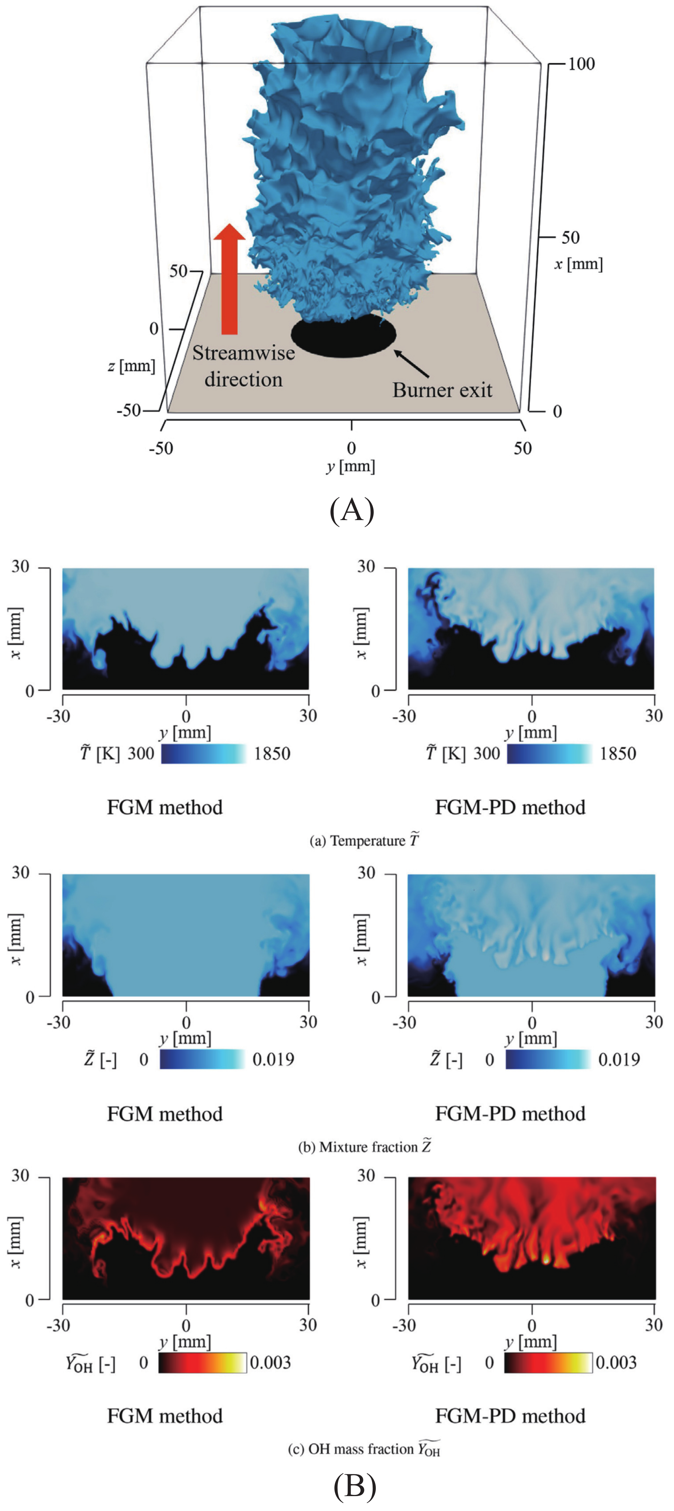
3.2. Effect of Diffusivity of Chemical Species

Most previous studies employing FPV methods have assumed that mass and heat diffuse at the same rate through the flame, i.e., the Lewis number ($Le$) is unity. However, when $Le$ is not 1, species and heat are redistributed locally. It is well-established that chemical species inherently have different diffusion rates (preferential diffusion effects), resulting in $Le$ values that are not necessarily unity, which can significantly impact flame stability [31,32].

The Lewis number ($Le$) is defined as the ratio of thermal diffusivity to mass diffusivity. Its value depends on the specific chemical species involved, as illustrated in

Table 1. Simplified transport model Lewis numbers [33].

Species	Value
${\mathrm{CH}}_4$	0.97
${\mathrm{O}}_2$	1.11
${\mathrm{H}}_2\mathrm{O}$	0.83
${\mathrm{CO}}_2$	1.39
$\mathrm{H}$	0.70
$\mathrm{O}$	0.73
$\mathrm{OH}$	1.10
${\mathrm{H}}_2$	0.30
$\mathrm{CO}$	1.10
${\mathrm{H}}_2{\mathrm{O}}_2$	1.12
$\mathrm{HCO}$	1.27
${\mathrm{CH}}_2\mathrm{O}$	1.28
${\mathrm{CH}}_3$	1.00
${\mathrm{CH}}_3\mathrm{O}$	1.30
${\mathrm{N}}_2$	1.00

[33], and is calculated as follows:

$$Le={\displaystyle \frac{\alpha }{D}},$$

(9)

where $\alpha$ is the thermal diffusivity in the gas mixture.

In many turbulent combustion simulations, the diffusion coefficient of each chemical species in the gaseous mixture is not calculated explicitly, and the Lewis number is assumed to be unity. This assumption is often justified because diffusion phenomena are highly influenced by the turbulent field, rendering molecular diffusion relatively insignificant. As such, assuming a Lewis number of unity is generally acceptable. However, special consideration is required when using hydrogen as a fuel or when a significant amount of hydrogen is generated during the reaction process [34].

Figure 7 presents a study of the combustion field of a lean, premixed H₂/air low-swirl lifted flame [35]. In this study, the preferential diffusion characteristics are expressed as the sum of the molecular diffusion coefficients of each chemical species, weighted by their mass fractions. This diffusion coefficient is then used to solve the conservation equations for the mixture fraction (Z) and the reaction progress variable (C). Figure 7B shows a comparison between the conventional FGM method and the FGM-PD (Preferential Diffusion) method, which accounts for the preferential diffusion of chemical species. The FGM-PD results reveal inhomogeneous distributions of $\tilde{T}$ and $\tilde{Z}$ near the flame front. Specifically, $\tilde{T}$ and $\tilde{Z}$ increase on the burnt gas side of convex regions and decrease on the concave regions facing the unburnt gas side. This behavior is caused by the preferential diffusion effect, where molecular diffusion of highly diffusive species, such as H₂, occurs from the unburnt to the burnt gas side. These species converge in convex regions of the flame front and diverge in concave regions, directly impacting the distribution of $\tilde{Z}$.

The approaches discussed so far have the drawback that the number of control variables connecting the physical combustion field and the flamelet database increases. In general, computers have several gigabytes of memory per CPU. However, when the number of control variables exceeds four, the database size can grow to tens of gigabytes, making it impractical to use high-dimensional flamelet databases. Recently, a few studies have explored compressing flamelet databases using deep learning techniques based on artificial neural networks (ANNs) [36,37]. ANN-based compression reduces the size of the original flamelet database to a fraction of its initial size or even to a few thousandths thereof.

Figure 8 presents the results of analyzing the Sydney methane–hydrogen/air flame (SMH1) [38] using a compressed flamelet database [36]. In Figure 8, the calculation results obtained employing the ANN method for temperature and water mass fraction show good agreement with experimental data at $x/D_{\mathrm{ref}}=1.1$ and 2.5 as other table calculations. The slight underprediction of the CO₂ mass fraction observed around $\tilde{Z}=0.25$ at $x/D_{\mathrm{ref}}=0.2$ is not attributed to the ANN method but, rather, to the strong sensitivity of CO₂ to the progress variable and small differences in $\tilde{C}$ between simulations employing the ANN method and those employing conventional tabulation techniques.

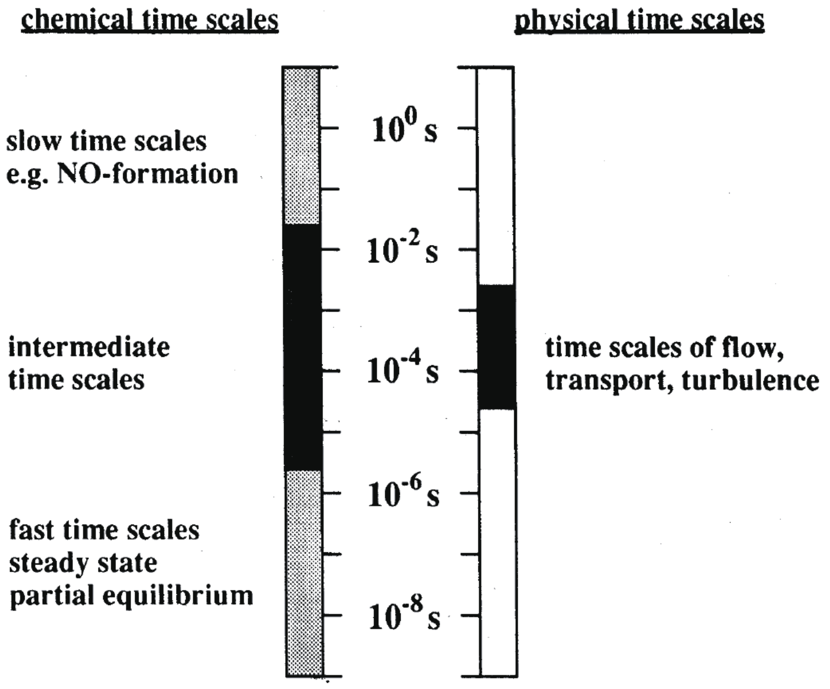
4. Applicability to Relatively Slow Reactions

In general, combustion flow fields involve processes ranging from rapid chain-branching reactions dominated by radicals to the slower formation of pollutants such as NOx [39] and soot [40], covering a very wide range of time scales, as shown in Figure 9 [41]. Wen et al. discovered that directly extracting the NO mass fraction from a flamelet library can lead to significant inaccuracies, particularly in the presence of fuel-bound NO. They recommended solving the transport equation for NO with a modified NO source term to achieve significantly more accurate NO predictions [42]. This method was adopted in this study, where the Favre-filtered transport equation for NO is solved in the flow field to account for NO emissions, as expressed in Equation (10).

$$\begin{array}{c}\hfill {\displaystyle \frac{\partial \overline{\rho }{\tilde{Y}}_{\mathrm{NO}}}{\partial t}}+{\displaystyle \frac{\partial \overline{\rho }\widetilde{u_j}{\tilde{Y}}_{\mathrm{NO}}}{\partial x_j}}={\displaystyle \frac{\partial }{\partial x_j}}\left\{\left({\displaystyle \frac{\mu }{Sc}}+{\displaystyle \frac{{\mu }_{sgs}}{S{c}_t}}\right){\displaystyle \frac{\partial {\tilde{Y}}_{\mathrm{NO}}}{\partial x_j}}\right\}+\overline{\rho }{\tilde{\dot{\omega }}}_{Y_{\mathrm{NO}}}\end{array}$$

(10)

The source term (${\tilde{\dot{\omega }}}_{Y_{\mathrm{NO}}}$) is calculated using the method proposed by Ihme and Pitsch [43], which accounts for both the production and rescaled consumption terms of forward and backward reactions, as described in Equation (11) [28,44].

$$\begin{array}{c}\hfill {\tilde{\dot{\omega }}}_{Y_{\mathrm{NO}}}={\tilde{\dot{\omega }}}_{Y_{\mathrm{NO}}}^{+}+{\tilde{Y}}_{\mathrm{NO}}{\displaystyle \frac{{\tilde{\dot{\omega }}}_{Y_{\mathrm{NO}}}^{-}}{{\tilde{Y}}_{\mathrm{NO}}^{flm}}}\end{array}$$

(11)

Figure 10 shows the results of analyzing combustion characteristics of the ammonia/coal co-firing. In Figure 10b, the 7D NA-FPV-LES (non-adiabatic FPV LES) model represents the case closest to the experimental conditions, while the 6D NA-FPV-LES model ignores the temperature differences in the supplied oxygen. The 5D AD-FPV-LES (adiabatic FPV LES) model further simplifies by ignoring the temperature differences in the supplied oxygen and assuming adiabatic conditions. The authors concluded that, due to the interaction of various phenomena, such as the recirculating flow generated by the swirling flow, heat loss caused by temperature differences, and chemical reactions, the 7D NA-FPV-LES approach provided improved predictions for the O₂ mole fraction and NO (ppm) profiles within the primary reaction zone—ranging from the burner outlet to the staged air introduction position—compared to the 6D NA-FPV-LES and 5D AD-FPV-LES cases.

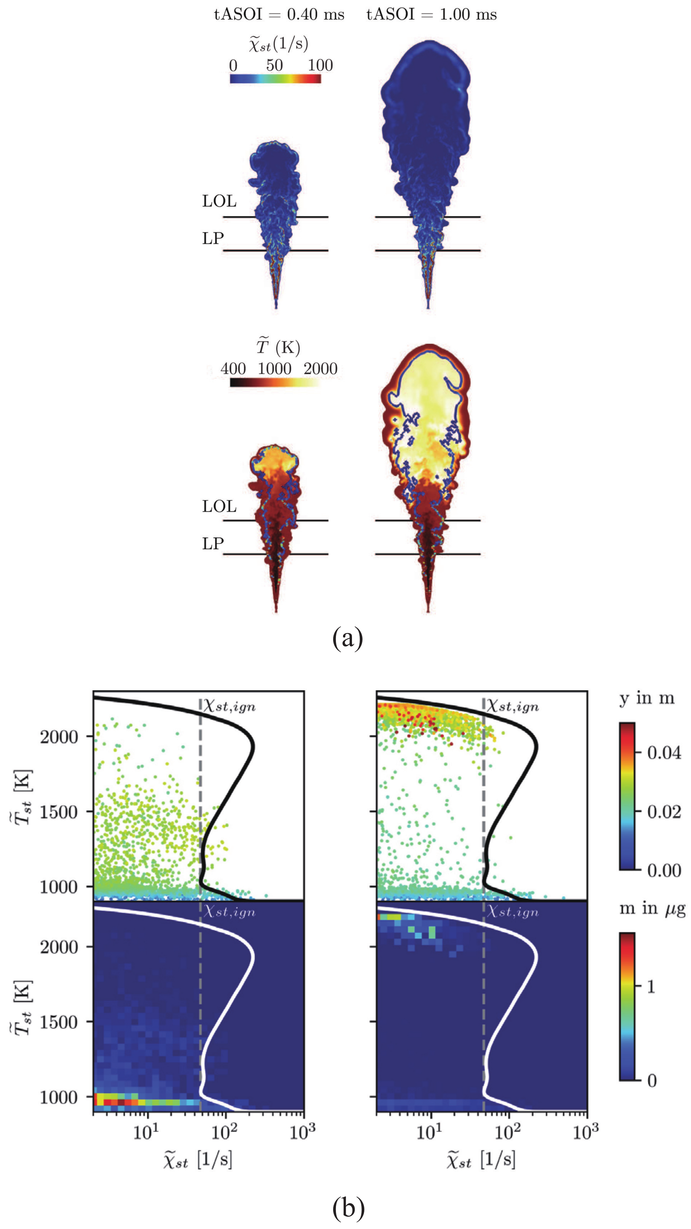
5. Consideration of Non-Stationary Phenomena

It is said that highly unsteady combustion phenomena, such as ignition and extinction, require consideration of unsteady reaction progress variables [45,46,47]. Typically, the steady solutions of the flamelet equations consist of both stable and unstable branches. Unsteady flamelet solutions are simulated for different scalar dissipation rates, starting from adiabatic mixing between fuel (mixture fraction, $Z=1$) and oxidizer ($Z=0$) until a steady-state solution is obtained [48,49]. These unsteady flamelet solutions are essential for capturing transient phenomena such as ignition and extinction.

Figure 11 illustrates a study of the ignition and extinction of ECN Spray A [50]. In Figure 11a, the penetration and lift-off length of the liquid fuel appear to agree with experimental results. However, when the temperature and scalar dissipation rate are extracted from this combustion flow field, the data deviate from the steady solution of the flamelet equation (solid line), as shown in Figure 11b. This deviation is attributed to unsteady extinction effects, suggesting that such effects need to be incorporated into the flamelet database in future studies.

6. Summary

This review paper provides an overview of recent advancements in tabulated chemistry models, with a focus on those based on the flamelet/progress-variable (FPV) method. In particular, it highlights scenarios involving multi-point fuel injection, the effects of heat loss in combustion flow fields, the influence of varying diffusion coefficients, and other complex phenomena. The three most important aspects of this review are summarized as follows.

• The flamelet/progress-variable (FPV) method has been successfully applied to a wide range of combustor scales, from laboratory experiments to practical applications, as well as across various fuel types, establishing itself as a critical tool for combustion analysis.
• By taking into account fluid dynamics and reaction kinetics factors, such as the non-adiabatic effect of the combustion field and the preferential diffusion of chemical species, FPV methods are able to analyze combustion phenomenon under a wide range of conditions.
• Attempts to reproduce basic phenomena such as ignition and extinction of the flame are also leading to progress in elucidating the fundamental physical phenomena.

References

1. Yamashita, H.; Shimada, M.; Takeno, T. A numerical study on flame stability at the transition point of jet diffusion flames. Symp. (Int.) Combust. 1996, 26, 27–34. [Google Scholar] [CrossRef]
2. Hara, T.; Muto, M.; Kitano, T.; Kurose, R.; Komori, S. Direct numerical simulation of a pulverized coal jet flame employing a global volatile matter reaction scheme based on detailed reaction mechanism. Combust. Flame 2015, 162, 4391–4407. [Google Scholar] [CrossRef]
3. Hwang, S.M.; Kurose, R.; Akamatsu, F.; Tsuji, H.; Makino, H.; Katsuki, M. Application of optical diagnostics techniques to a laboratory-scale turbulent pulverized coal flame. Energy Fuels 2005, 19, 382–392. [Google Scholar] [CrossRef]
4. van Oijen, J.A.; de Goey, L.P.H. Modelling of premixed laminar flames using flamelet-generated manifolds. Combust. Sci. Technol. 2000, 161, 113–137. [Google Scholar] [CrossRef]
5. Gupta, H.; Teerling, O.J.; van Oijen, J.A. Effect of progress variable definition on the mass burning rate of premixed laminar flames predicted by the Flamelet Generated Manifold method. Combust. Theory Model. 2021, 25, 631–645. [Google Scholar] [CrossRef]
6. Pierce, C.D.; Moin, P. Progress-variable approach for large-eddy simulation of non-premixed turbulent combustion. J. Fluid Mech. 2004, 504, 73–97. [Google Scholar] [CrossRef]
7. Pitsch, H. Flamemaster: A C++ Computer Program for 0D Combustion and 1D Laminar Flame Calculations. 1998. Available online: https://www.itv.rwth-aachen.de/downloads/flamemaster (accessed on 28 January 2025).
8. Ma, T.; Gao, Y.; Kempf, A.M.; Chakraborty, N. Validation and implementation of algebraic LES modelling of scalar dissipation rate for reaction rate closure in turbulent premixed combustion. Combust. Flame 2014, 161, 3134–3153. [Google Scholar] [CrossRef]
9. Ruan, S.; Swaminathan, N.; Isono, M.; Saitoh, T.; Saitoh, K. Simulation of premixed combustion with varying equivalence ratio in gas turbine combustor. J. Propuls. Power 2015, 31, 861–871. [Google Scholar] [CrossRef]
10. Chen, Z.X.; Ruan, S.; Swaminathan, N. Large eddy simulation of flame edge evolution in a spark-ignited methane-air jet. Proc. Combust. Inst. 2017, 36, 1645–1652. [Google Scholar] [CrossRef]
11. Ghiasi, G.; Doan, N.A.K.; Swaminathan, N.; Yennerdag, B.; Minamoto, Y.; Tanahashi, M. Assessment of SGS closure for isochoric combustion of hydrogen-air mixture. Int. J. Hydrogen Energy 2018, 43, 8105–8115. [Google Scholar] [CrossRef]
12. Swaminathan, N.; Bai, X.-S.; Brethouwer, G.; Haugen, N.E.L.; Fureby, C.; Brethouwer, G. (Eds.) Advanced Turbulent Combustion Physics and Applications; Cambridge University Press: Cambridge, UK, 2022. [Google Scholar]
13. Rieth, M.; Clements, A.G.; Rabaçal, M.; Proch, F.; Stein, O.T.; Kempf, A.M. Flamelet LES modeling of coal combustion with detailed devolatilization by directly coupled CPD. Proc. Combust. Inst. 2017, 36, 2181–2189. [Google Scholar] [CrossRef]
14. Mayrhofer, M.; Koller, M.; Seemann, P.; Bordbar, H.; Prieler, R.; Hochenauer, C. MILD combustion of hydrogen and airean efficient modelling approach in CFD validated by experimental data. Int. J. Hydrogen Energy 2022, 47, 6349–6364. [Google Scholar] [CrossRef]
15. Wen, J.; Hu, Y.; Nishiie, T.; Iino, J.; Masri, A.; Kurose, R. A flamelet LES of turbulent dense spray flame using a detailed high-resolution VOF simulation of liquid fuel atomization. Combust. Flame 2022, 237, 111742. [Google Scholar] [CrossRef]
16. Kong, F.; Li, T.; Cheng, C.; Shan, C.; Xu, B. Modeling of spray flame in gas turbine combustors with LES and FGM. Fuel 2022, 325, 124756. [Google Scholar] [CrossRef]
17. Kasuya, H.; Iwai, Y.; Itoh, M.; Morisawa, Y.; Nishiie, T.; Kai, R.; Kurose, R. Les/flamelet/ANN of oxy-fuel combustion for a supercritical CO2 power cycle. Appl. Energy Combust. Sci. 2022, 12, 100083. [Google Scholar] [CrossRef]
18. Albrecht, B.; Zahirovic, S.; Bastiaans, R.; van Oijen, J.A.; de Goey, L.P.H. A premixed flamelet-PDF model for biomass combustion in a grate furnace. Energy Fuels 2008, 22, 1570–1580. [Google Scholar] [CrossRef]
19. Sakib, A.H.M.N.; Farokhi, M.; Birouk, M. Evaluation of flamelet-based partially premixed combustion models for simulating the gas phase combustion of a grate firing biomass furnace. Fuel 2023, 333, 126343. [Google Scholar] [CrossRef]
20. Baba, Y.; Kurose, R. Analysis and flamelet modelling for spray combustion. J. Fluid Dyn. 2008, 612, 45–79. [Google Scholar] [CrossRef]
21. Watanabe, J.; Yamamoto, K. Flamelet model for pulverized coal combustion. Proc. Combust. Inst. 2015, 35, 2315–2322. [Google Scholar] [CrossRef]
22. Peters, N. Laminar diffusion flamelet models in non-premixed turbulent combustion. Prog. Energy Combust. Sci. 1984, 10, 319–339. [Google Scholar] [CrossRef]
23. Wen, X.; Shamooni, A.; Zirwes, T.; Stein, O.T.; Kronenburg, A.; Hasse, C. Carrier-phase direct numerical simulation and flamelet modeling of NOx formation in a pulverized coal/ammonia co-firing flame. Combust. Flame 2024, 269, 113722. [Google Scholar]
24. Wen, X.; Luo, K.; Jin, H.; Fan, J. Large eddy simulation of piloted pulverised coal combustion using extended flamelet/progress variable model. Combust. Theory Model. 2017, 21, 925–953. [Google Scholar]
25. Meller, D.; Lipkowicz, T.; Rieth, M.; Stein, O.T.; Kronenburg, A.; Hasse, C.; Kempf, A.M. Numerical analysis of a turbulent pulverized coal flame using a flamelet/progress variable approach and modeling experimental artifacts. Energy Fuels 2021, 35, 7133–7143. [Google Scholar] [CrossRef]
26. Proch, F.; Kempf, A.M. Modeling heat loss effects in the large eddy simulation of a model gas turbine combustor with premixed flamelet generated manifolds. Proc. Combust. Inst. 2015, 35, 3337–3345. [Google Scholar]
27. Kishimoto, A.; Moriai, H.; Takenaka, K.; Nishiie, T.; Adachi, M.; Ogawara, A.; Kurose, R. Application of a nonadiabatic flamelet/progress-variable approach to Large-eddy simulation of H2/O2 combustion under a pressurized condition. J. Heat Transf. 2017, 139, 124501-1. [Google Scholar] [CrossRef]
28. Yadav, S.; Yu, P.; Tanno, K.; Watanabe, H. Multi-stream FPV-LES modeling of ammonia/coal co-firing on a semi-industrial scale complex burner with pre-heated secondary, tertiary, and staged combustion air. Combust. Flame 2024, 270, 113729. [Google Scholar]
29. Tucker, P.; Menon, S.; Merkle, C.; Oefelein, J.; Yang, V. Validation of high-fidelity CFD simulations for rocket injector design. In Proceedings of the 44th AIAA/ASME/SAE/ASEE Joint Propulsion Conference & Exhibit, Hartford, CT, USA, 21–23 July 2008. [Google Scholar]
30. Pal, S.; Marshall, W.; Woodward, R.; Santoro, R. Wall heat flux measurements for a uni-element GO2/GH2 shear coaxial injector. In Proceedings of the Third International Workshop on Rocket Combustion Modeling, Paris, France, 13 March 2006. [Google Scholar]
31. Pitsch, H.; Peters, N. A consistent Flamelet formulation for non-premixed combustion considering differential diffusion effects. Combust. Flame 1998, 114, 26–40. [Google Scholar]
32. Donini, A.; Bastiaans, R.J.M.; van Oijen, J.A.; de Goey, L.P.H. Differential diffusion effects inclusion with flamelet generated manifold for the modeling of stratified premixed cooled flames. Proc. Combust. Inst. 2015, 35, 831–837. [Google Scholar]
33. Smooke, M.D. Reduced Kinetic Mechanisms and Asymptotic Approximations for Methane-Air Flames: A Topical Volume; Springer: Berlin/Heidelberg, Germany, 1991. [Google Scholar]
34. Altantzis, C.; Frouzakis, C.E.; Tomboulides, A.G.; Matalon, M.; Boulouchos, K. Hydrodynamic and thermodiffusive instability effects on the evolution of laminar planar lean premixed hydrogen flames. J. Fluid Mech. 2012, 700, 329–361. [Google Scholar]
35. Kai, R.; Tokuoka, T.; Nagao, J.; Pillai, A.L.; Kurose, R. LES flamelet modeling of hydrogen combustion considering preferential diffusion effect. Int. J. Hydrogen Energy 2023, 48, 11086–11101. [Google Scholar]
36. Ihme, M.; Schmitt, C.; Pitsch, H. Optimal artificial neural networks and tabulation methods for chemistry representation in LES of a bluff-body swirl-stabilized flame. Proc. Combust. Inst. 2009, 32, 1527–1535. [Google Scholar]
37. Honzawa, T.; Kai, R.; Hori, K.; Seino, M.; Nishiie, T.; Kurose, R. Experimental and numerical study of water sprayed turbulent combustion: Proposal of a neural network modeling for five-dimensional flamelet approach. Energy AI 2021, 5, 100076. [Google Scholar] [CrossRef]
38. Masri, A.R. Web Site for the Sydney Swirl Flame Series. 2006. Available online: http://www.aeromech.usyd.edu.au/thermofluids (accessed on 28 January 2025).
39. Wen, X.; Berger, L.; vom Lehn, F.; Parente, A.; Pitsch, H. Numerical analysis and flamelet modeling of NOx formation in a thermodiffusively unstable hydrogen flame. Combust. Flame 2023, 253, 112817. [Google Scholar] [CrossRef]
40. Wick, A.; Attili, A.; Bisetti, F.; Pitsch, H. DNS-driven analysis of the Flamelet/Progress Variable model assumptions on soot inception, growth, and oxidation in turbulent flames. Combust. Flame 2020, 214, 437–449. [Google Scholar] [CrossRef]
41. Maas, U.; Pope, S.B. Simplifying chemical kinetics: Intrinsic low-dimensional manifolds in composition space. Combust. Flame 1992, 88, 239–264. [Google Scholar] [CrossRef]
42. Wen, X.; Debiagi, P.; Stein, O.T.; Kronenburg, A.; Kempf, A.M.; Hasse, C. Flamelet tabulation methods for solid fuel combustion with fuel-bound nitrogen. Combust. Flame 2019, 209, 155–166. [Google Scholar] [CrossRef]
43. Ihme, M.; Pitsch, H. Modeling of radiation and nitric oxide formation in turbulent nonpremixed flames using a flamelet/progress variable formulation. Phys. Fluids 2008, 20, 055110. [Google Scholar] [CrossRef]
44. Wan, J.; Guo, J.; Wei, Z.; Jiang, X.; Liu, Z. Large eddy simulation of NO formation in non-premixed turbulent jet flames with flamelet/progress variable approach. J. Therm. Sci. 2024, 33, 2399–2412. [Google Scholar] [CrossRef]
45. Pitsch, H.; Ihme, M. An unsteady/flamelet progress variable method for les of nonpremixed turbulent combustion. In Proceedings of the 43rd AIAA Aerospace Sciences Meeting and Exhibit Meeting Papers, Reno, NV, USA, 10–13 January 2005; p. 2004-557. [Google Scholar]
46. Ihme, M.; See, Y.C. Prediction of autoignition in a lifted methane/air flame using an unsteady flamelet/progress variable model. Combust. Flame 2010, 157, 1850–1862. [Google Scholar]
47. Bajaj, C.; Ameen, M.; Abraham, J. Evaluation of an unsteady flamelet progress variable model for autoignition and flame lift-off in diesel jets. Combust. Sci. Technol. 2013, 185, 454–472. [Google Scholar]
48. Sun, Z.; Gierth, S.; Pollack, M.; Hasse, C.; Scholtissek, A. Ignition under strained conditions: Unsteady flamelet progress variable modeling for diesel engine conditions in the transient counterflow configuration. Combust. Flame 2021, 240, 111841. [Google Scholar] [CrossRef]
49. Gierth, S.; Haspel, P.; Scholtissek, A.; Sun, Z.; Popp, S.; Hasse, C. Evaluation of the unsteady flamelet progress variable approach in Large Eddy Simulations of the ECN Spray A. Sci. Technol. Energy Transit. 2022, 77, 5. [Google Scholar] [CrossRef]
50. Pickett, L.M. Engine Combustion Network, Sandia National Laboratory. 2013. Available online: https://ecn.sandia.gov (accessed on 28 January 2025).
Figure 1. Instantaneous distributions of flame index values in pulverized coal flame. This figure is adapted from Hara et al. [2].
Fluids 10 00083 g001
Figure 2. Example database of mass fractions of OH ( Y OH ), an intermediate species in the combustion of hydrogen-containing fuels, tabulated with mixture fractions and reaction progress variables.
Fluids 10 00083 g002
Figure 3. Schematic diagram of data interaction between physical space and Z space. This figure is adapted from Baba and Kurose [20].
Fluids 10 00083 g003
Figure 4. The study of the spray-jet flame using the flamelet/progress-variable method. (A) Schematic of the computational domain and inlet conditions. (B) Comparison of instantaneous distribution of gaseous temperature ( T * ). (a) LAR (Arrhenius formulation); (b) LFM (steady flamelet); (c) LFMM (modified steady flamelet; C = Y CO 2 + Y H 2 O ); (d) LFM-P (flamelet/progress-variable; C = h ); (e) LFM-E (flamelet/progress-variable). These figures are adapted from Baba and Kurose [20].
Fluids 10 00083 g004
Figure 5. The study of the pulverized coal/ammonia co-firing flame in the turbulent mixing layer. (a) Schematic of the computational setup. The white dots represent the pulverized coal particles at the initial time instant. (b) Instantaneous contours of various mixture fractions of Z v o l , Z p r o , Z p i l , and Z a m in the turbulent mixing layer at t = 3.3 ms . The temperature iso-surfaces correspond to T = 1940 K , corresponding to the peak temperature of the NH3/air mixture. The iso-surfaces are colored according to the local value of Y NO . A total of 8000 sample coal particles colored according to their temperatures are superimposed. These figures are adopted from Wen et al. [23].
Fluids 10 00083 g005
Figure 6. The study of the H 2 / O 2 combustion in the coaxial combustor at Pennsylvania State University [29,30]. (a) Schematics of the computational domain and conditions. (b) Comparison of the streamwise profile of time-averaged wall heat flux ( q ˜ wall ) among predicted values obtained by FPV and NA-FPV methods and measured values. These figures are adopted from Kishimoto et al. [27].
Fluids 10 00083 g006
Figure 7. The study of the combustion field of the lean, premixed H2/air low-swirl lifted flame. (A) Instantaneous distribution of the iso-surface of gas temperature ( T ˜ ) at 1500 K (colored in blue) above the y z plane (i.e., the burner exit plane ( x = 0 mm), colored in gray) obtained by the FGM-PD method, with the burner exit represented by the black elliptical patch. (B) Comparisons of instantaneous distributions of (a) gas temperature ( T ˜ ), (b) mixture fraction, ( Z ˜ ), and (c) OH mass fraction ( Y OH ˜ ) at z = 0 mm between the conventional FGM method (left) and the FGM-PD method (right). These figures are adopted from Kai et al. [35].
Fluids 10 00083 g007
Figure 8. Comparison of measured and calculated mixture fraction-conditioned data for temperature and mass fractions of H 2 O and CO 2 at different axial locations in the Sydney SMH1 flame [38]. This figure is adopted from Ihme et al. [36].
Fluids 10 00083 g008
Figure 9. Characteristic time scales in turbulent reactive flows. This figure is adapted from Maas and Pope [41].
Fluids 10 00083 g009
Figure 10. The study of ammonia/coal co-firing on a semi-industrial-scale complex burner. (a) A schematic illustration of the computational domain, including an enlarged view of the burner. (b) Comparison of 7D NA-FPV-LES model prediction for temperature (top), O2 mole fraction ( X O 2 ) (mid), and NO mole fraction ( X NO ) (bottom), with experimental data and results from the 6D NA-FPV-LES and 5D AD-FPV-LES models for ammonia injection into the burner (left) and 1.0 m downstream (right). These figures are adopted from Yadav et al. [28].
Fluids 10 00083 g010
Figure 11. The study of the ignition of the ECN Spray A. (a) Distribution of the scalar dissipation rates under stoichiometric conditions ( χ ˜ s t ) used for table look-up (top row), and temperature ( T ˜ ) overlaid by the iso-line of Z ˜ = Z ˜ s t colored according to the χ ˜ s t (bottom row). The black horizontal lines denote the experimentally obtained liquid penetration (LP) of 9.6 mm and the steady lift-off length (LOL) of 16.1 mm. (b) Scatter plot of the temperature under stoichiometric conditions ( T ˜ s t = T ˜ ( Z ˜ s t ) ) over the corresponding scalar dissipation rate ( χ ˜ s t ), colored according to the axial distance to the nozzle (top row) and the corresponding mass distribution (bottom row). These figures are adopted from Gierth et al. [49].
Fluids 10 00083 g011