Development of a Lagrangian Temperature Particles Method to Investigate the Flow Around a Rough Bluff Body

Abstract

This paper presents a roughness surface model for Lagrangian simulations that interacts with both temperature and vorticity fields. The chosen problem is the uniform flow around a rough circular cylinder heated with constant temperature under mixed convection. The methodology used is the Temperature Particles Method (TPM), in which both vorticity and temperature fields are discretized in particles to simulate the real flow in a purely Lagrangian form. The simulation is computationally extensive due to the application of the Biot–Savart law for the two fields and the calculation of buoyancy forces, which is alleviated by the use of parallel programming with OpenMP. The simulation of roughness effects for both fields is obtained using a Large Eddy Simulation (LES) model for vorticity, based on the second-order velocity structure function, which is correlated with the thermal diffusivity through the turbulent Prandtl number. In general, the results indicate that roughness increases the drag coefficient, while an increase in the Richardson number reduces this coefficient.

1. Introduction

The flow around bluff bodies is characterized by the separation of a significant portion of the boundary layer, leading to the formation of a wake. In engineering structures, this wake formation can result in the phenomenon of lock-in, where flow-induced vibrations synchronize with the structure’s natural frequency, potentially causing structural failure. To prevent such failures, the field of wake suppression has garnered significant interest in recent years, with Rashidi [1] considering three different approaches of suppression: (a) active control methods; (b) passive control methods; and (c) control by employing an external element. This paper will consider the combined effects of surface roughness (a passive control method) and thermal effects (an active control method), specifically assessing the influence of surface roughness on heat transfer and drag coefficients when they are present simultaneously in a fluid flow problem.

Combined effects are present in several industrial and practical applications, leading to the need for better understand them and have models that can predict the structural response. For example, risers from the oil industry tend to increase surface roughness as they age. In the same way, marine structures can have increased roughness as shellfish start living in them. The added effects of a heated surface are useful to understand how shell and tube heat exchangers will respond as the surface rusts or suffers from incrustation. Al-Rubaiy [2] studied these interactions around a circular cylinder in an experimental setup and how flow turbulence influences the aerodynamic forces and Nusselt number. Increases in surface roughness typically increases drag, but when considering bluff bodies, it can lead to a change in the flow regimen and result in the anticipation of the drag crisis, making the prediction of this flow complex. Dhiman and Dwivedi [3] studied the effects of the Richardson number and the gap between two heated cylinders with a constant temperature and Re = 100, showing that the heat transfer changes drastically the flow dynamics. This study considered smooth surfaces and observed slight increases in the drag coefficient. Afgan et al. [4] studied the flow around two smooth heated cylinders in tandem at Re = 3000, investigating the influences of gap ratios and heat transfer in the lift, drag, and pressure coefficients and in the Nusselt number. However, simulations considering both heating and roughness effects are scarce in the literature, and numerical simulations typically work at lower Reynolds values due to the diffusive problem that exists at higher values when using Eulerian methods.

Numerical approaches are useful to simulate wake suppression without needing prohibitive prototype costs, where both Eulerian or Lagrangian methods could be used to simulate flow dynamics. Lagrangian description is useful when compared to approaches which use meshes because they can represent the flow faithfully in regions of strain and do not require setting boundary conditions over the domain. The first application of the Discrete Vortex Method (DVM) considering viscous forces was proposed by Chorin [5], where the author simulated the flow around a circular cylinder considering a slightly viscous flow and used the Random Walk method to simulate the diffusion. Smith and Stansby [6] simulated the temperature field with the vorticity field for the first time in a formulation similar to the DVM, which became known as the Temperature Particles Method (TPM). This formulation assumed forced heat transfer from the cylinder to the fluid, as no model of buoyancy had been developed at the time, with Ogami [7] presenting two different approaches to simulate the vortex–temperature interactions.

Since then, several contributions have been made to the DVM, including different models for the diffusion scheme [8,9,10,11,12,13,14] and ways to reorganize the vorticity field to circumvent Lagrangian distortion [15,16]. In parallel to theoretical considerations and advances, in the past years, several researchers have applied the DVM to engineering applications, considering new effects and how to simulate them numerically. The use of a Lagrangian description is advantageous because of different factors such as (a) there is no mesh in a typical simulation; therefore, there is no need to stipulate boundary conditions on the inlet or outlet of a mesh, nor is there a need to create and refine a mesh and execute mesh independence tests; (b) the properties of interest (like temperature and vorticity) are independently tracked as the time steps increase, which allows for massive parallelization of the numerical code; (c) at every moment in the simulation, the velocity field for both the vortex blobs and temperature particles is directly calculated via the Biot–Savart law. Due to the material derivative, it is not necessary to calculate advective derivatives, and (d) as an extension, since the velocity field is known at every instant, an LES formulation using the second-order velocity structure function is suitable for the method and easy to implement numerically. In addition to that, the use of LES turbulence modeling allows for the simulation of surface roughness effects [17] that can be extended to the temperature field, which is the focus of this paper.

Turbulence modeling is a defining factor when considering flows with higher Reynolds numbers. Since turbulence is a three-dimensional phenomena, only a few authors have implemented a two-dimensional model to consider the turbulent fluctuations in their works: First, we note the adaptation of the second-order velocity structure function made by Alcântara Pereira [18], which uses the known velocity at every discrete vortex blob, a characteristic of Lagrangian methods, to calculate the local eddy viscosity and account for turbulence effects. A second implementation was made by Prendergast [19], which was also used by [20], consisting of adding discrete vortices once every few time steps to simulate the turbulent velocity fluctuations. However, those studies focused on the vorticity field; recently, Chiaradia et al. [21] adapted the former approach to consider the turbulent thermal diffusivity on the temperature particles using the velocity fluctuations given by the vorticity field.

The influence of roughness effects in the flow around a cylinder was shown by Achenbach and Heinecke [22] for a wide range of Reynolds numbers (Re). The experiments revealed that the drag and Strouhal number can either reduce or increase depending on the Reynolds number. In a more recent study, Tian et al. [23] studied different roughness shapes and heights on the flow past a circular cylinder in a large recirculating tank where $Re$ ranged from 40,000 to 200,000. The results showed that the drag coefficient consistently increased with increasing roughness heights. A similar experiment [24] considered the roughness effects of mussels in the hydrodynamical forces around a circular cylinder using an experimental setup wherein the Reynolds number ranged from 0.5–4.0 $\times {10}^4$, and the authors observed a drag increase at constant Reynolds numbers as the relative roughness surface increased from 0 to 0.136. Also, the roughness delayed the drag crisis in their tests, as well as the reduction in the Strouhal number. Sun et al. [25] explored different roughness heights and observed a reduction in the Strouhal number as surface roughness increased on the flow past a circular cylinder, attributing this to the forward movement of the separation point.

In previous works, our group developed a DVM capable of modeling surface roughness effects [17] and employed a model proposed by Ogami [7] to simulate the effects of natural convection in the dissipation of aircraft wingtip vortices [26]. Recently, the effects of mixed convection were further developed to implement a Large-Eddy Simulation (LES) model into the temperature particles clutter using the Temperature Particles Method (TPM) [21].

In this work, the TPM is employed to solve the Navier–Stokes equations using a two-dimensional turbulence model with a LES approach and considering both effects of mixed convection and surface roughness to simulate the flow around a circular cylinder. This initial approach serves by proposing a novel model that accounts for the effects of the surface roughness on the thermal boundary layer.

The surface is represented using the Panels Method [27] whereby the cylinder is substituted by a distribution of sources of uniform density along a polygon inscripted to the circle. The Panels Method was developed as a potential theory tool, hence the need to use a diffusion scheme to simulate a viscous flow. In this paper, we opted to use the Random Walk Method [5] due to its simplicity and suitability at higher Reynolds numbers. Before the diffusion and advection processes, it is necessary to evaluate the local eddy viscosity at every computational point (vortex blobs and temperature particles). The LES approach is unique in the sense that while the large eddies (low frequencies) are simulated by vortex and temperature clouds, i.e., by the numerical method, the small eddies’ (high frequencies) interactions with the larger scales need to be modeled [28].

The thermal effects are simulated using a direct interpretation of Fourier’s law [26], using it to generate temperature particles at shedding points on a panel. Said particles will receive velocity inductions from vortex blobs and populate the wake. The mixed convection is determined by the influence of each temperature particle on every vortex blob [7], where the temperature inductions to the left and right result in buoyancy forces translated as an increase in each vortex blob intensity. As one can notice, the calculations become progressively more demanding of the machine as the number of particles in the boundary layer and wake increases. This is explained by the complexity of $\mathcal{O}\left(Z^2\right)$ for a cloud consisting of Z particles interacting with each other, with vortex blobs inducing velocity to other vortices and temperature particles, while the temperature blobs induce temperature to each vortex blob during the natural convection effects. Due to this, it is necessary to adopt parallel programming using OpenMP on the in-house FORTRAN code.

2. Methodology

2.1. Mathematical Formulation

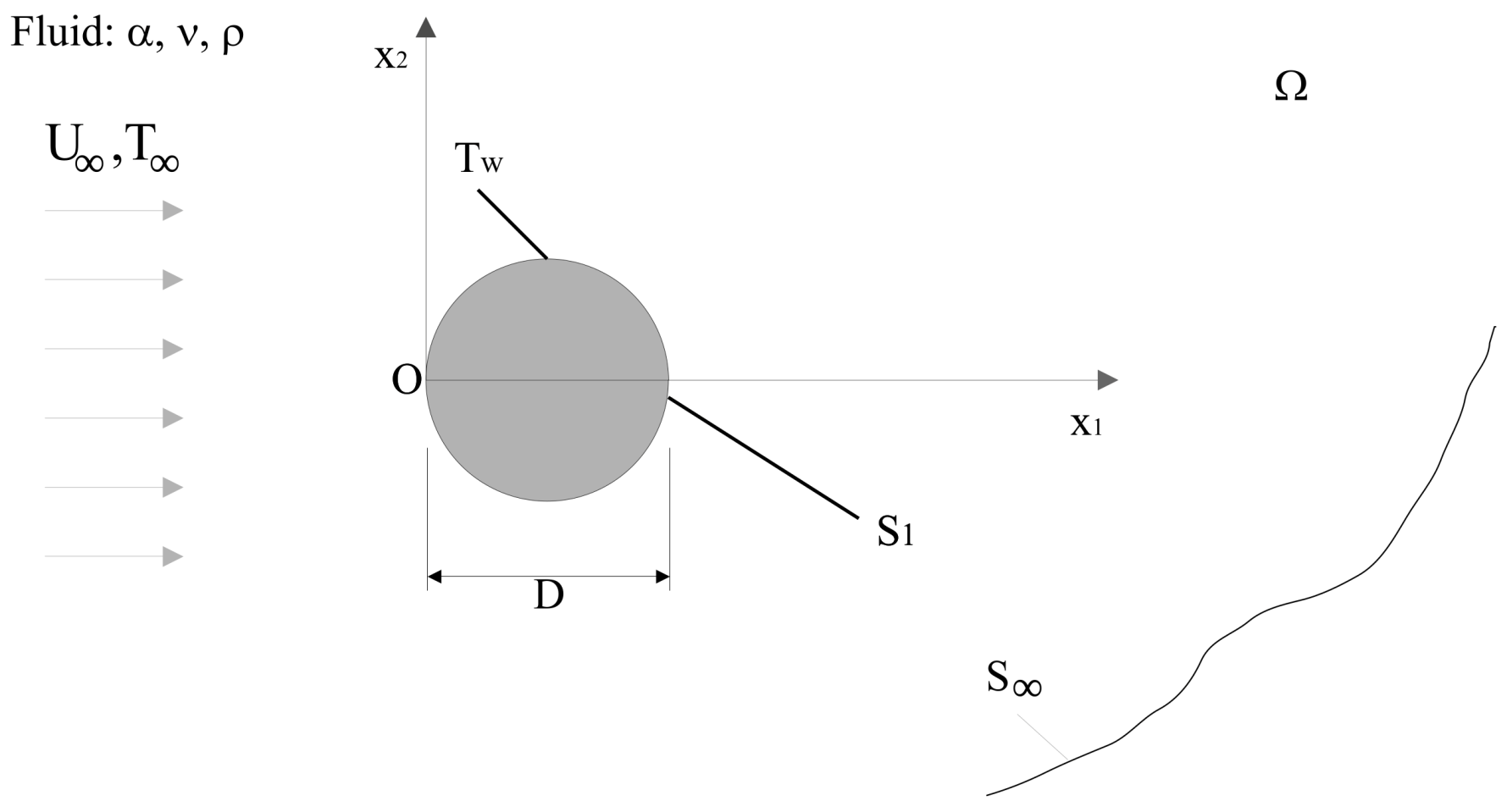
The geometry used to simulate the present problem is shown in Figure 1. There is an incident flow with velocity $U_{\infty }$ and temperature $T_{\infty }$ past a cylinder with diameter D. The cylinder is heated with a constant temperature $T_w$, and the wall has a roughness height $\epsilon$, while the contour constitutes surface $S_1$. The faraway boundary, $S_{\infty }$, is set on ‘the infinity’ to represent the boundary conditions on the far field. Therefore, the fluid domain is defined as $\Omega =S_1\cup S_{\infty }$. The boundary conditions on $S_1$ are the no-slip condition (the tangential velocity at $S_1$ equals to zero), the impermeability condition (the normal velocity at $S_1$ equals to zero) and the constant temperature condition on the wall ($T=T_w$ at $S_1$). The faraway boundary condition is the undisturbed flow: at $S_{\infty }$, the velocity of the flow equals to $U_{\infty }$.

We assume a two-dimensional, incompressible, and unsteady flow, a Newtonian fluid with kinematic viscosity $\nu$, a thermal diffusivity $\alpha$, a density $\rho$, and a thermal expansion coefficient $\beta$ that is allowed to change its density due to buoyancy effects, i.e., via the Boussinesq approximation [29]. The mathematical formulations for transporting vorticity (with roughness effects) and heat (with buoyancy forces) are detailed in Bimbato et al. [17] and Chiaradia et al. [21], respectively. Considering this approximation, applying the curl operator to the Navier–Stokes equations, and considering a LES turbulence model, the vorticity transport equation can be written as follows [21]:

$${\displaystyle \frac{D\overline{\omega }}{Dt}}={\displaystyle \frac{\partial \overline{\omega }}{\partial t}}+{\displaystyle \frac{\partial {\overline{u}}_j\overline{\omega }}{\partial x_j}}=\left({\displaystyle \frac{1}{Re}}+{\nu }_T\right){\displaystyle \frac{{\partial }^2\overline{\omega }}{\partial x_j{x}_j}}+Ri{\displaystyle \frac{\partial \overline{\theta }}{\partial x_j}},$$

(1)

where $D/Dt$ is the material derivative; $\overline{\omega }$ is the filtered vorticity field, treated as a scalar because the fluid domain is assumed two-dimensional; ${\nu }_T$ is the eddy viscosity coefficient; and the non-dimensional values $Re$, $Ri$, and $\overline{\theta }$ are defined as follows:

$$Re={\displaystyle \frac{U_{\infty }D}{\nu }},$$

(2)

$$Ri={\displaystyle \frac{g\beta (T_w-T_{\infty })D}{U_{\infty }^2}},$$

(3)

$$\overline{\theta }={\displaystyle \frac{\overline{T}-T_{\infty }}{T_w-T_{\infty }}}.$$

(4)

The energy equation is presented in the following manner:

$${\displaystyle \frac{D\overline{\theta }}{Dt}}={\displaystyle \frac{\partial \overline{\theta }}{\partial t}}+{\displaystyle \frac{\partial {\overline{u}}_j\overline{\theta }}{\partial x_j}}={\displaystyle \frac{\partial }{\partial x_j}}\left[\left({\displaystyle \frac{1}{RePr}}+{\displaystyle \frac{{\nu }_T}{ReP{r}_T}}\right){\displaystyle \frac{\partial \overline{\theta }}{\partial x_j}}\right],$$

(5)

where $Pr$ is the Prandtl number and $P{r}_T$ is the turbulent Prandtl number, defined as follows:

$$Pr={\displaystyle \frac{\nu }{\alpha }},$$

(6)

$$P{r}_T={\displaystyle \frac{{\nu }_T}{{\alpha }_T}}.$$

(7)

In Equation (7), ${\alpha }_T$ is the turbulent thermal diffusivity. $P{r}_T$ assumes a constant value of 0.95 [28]. It is clear that the constant value assumption simplifies the calculation of the thermal diffusivity coefficient since it can be obtained by a division of the local eddy viscosity coefficient by $P{r}_T$.

The eddy viscosity coefficients are obtained using a second-order velocity structure function proposed in the following [28]:

$${\nu }_T(\mathit{x},▵,t)=0.105C_k^{-3/2}▵\sqrt{{\overline{F}}_2(\mathit{x}\mathbf{,}\mathbf{▵}\mathbf{,}\mathit{t})},$$

(8)

where $C_k=1.4$ is the Kolmogorov constant, $▵$ is a representative length, and ${\overline{F}}_2$ is the second-order velocity structure function:

$${\overline{F}}_2(\mathit{x},▵,t)={\parallel \overline{\overline{\mathit{u}}(\mathit{x},t)-\overline{\mathit{u}}(\mathit{x}+\mathit{r},t)}\parallel }_{\parallel \mathit{r}\parallel =▵}^2.$$

(9)

In the three-dimensional formulation of ${\overline{F}}_2$ in Equation (9), the velocity fluctuations at spacial position $\mathit{x}$ are calculated only in points located at the surface of a sphere of radius $▵$, simulating the cutoff value for this type of LES model. In order to adapt this formulation for a two-dimensional Lagrangian approach, Alcântara Pereira [18] considered the velocity fluctuations inside an annular region, ensuring that very close particles do not induce velocity in each other, in agreement with the original formulation from [28]. The numerical approach to compute vorticity in each annular region containing vortex blobs is presented in [17].

The advantage of using the formulation presented here is that it does not use derivatives to obtain the local eddy viscosity coefficient. Also, the roughness will be considered a source of momentum on the boundary layer; therefore, the geometry does not need to be altered for different roughness heights, being translated instead as a change in the local eddy viscosity coefficient (see Section 2.2.3). Also, since we consider a constant turbulent Prandtl number, the turbulent thermal diffusion is also easily obtained from the local eddy viscosity coefficient.

Once the flow velocity field has been calculated, to recuperate the pressure field, which is lost after obtaining the vorticity transport equation, it is possible to use the divergence operator on the Navier–Stokes equations and to solve a Poisson equation for the pressure. This approach was proposed by Shintani and Akamatsu [30], and the final form of the equation is as follows:

$$\begin{array}{cc}\xi \tilde{Y}\left({\mathit{x}}^{\mathbf{\prime }}\right)+{\oint }_{S_1}{\displaystyle \frac{1}{2\pi }}{\displaystyle \frac{n_x(x-x^{\prime })+n_y(y-y^{\prime })}{{(x-x^{\prime })}^2+{(y-y^{\prime })}^2}}\tilde{Y}dS=\hfill & -{\int \int }_{\Omega }{\displaystyle \frac{\omega }{2\pi }}{\displaystyle \frac{v(x-x^{\prime })-u(y-y^{\prime })}{{(x-x^{\prime })}^2+{(y-y^{\prime })}^2}}d\Omega +\hfill \\ \hfill & -{\displaystyle \frac{1}{Re}}{\oint }_{S_1}{\displaystyle \frac{\omega }{2\pi }}{\displaystyle \frac{n_y(x-x^{\prime })-n_x(y-y^{\prime })}{{(x-x^{\prime })}^2+{(y-y^{\prime })}^2}}dS,\hfill \end{array}$$

(10)

where $\xi$ equals 1 in the fluid domain and ½ in the solid surface, $\tilde{Y}$ is the specific work (necessary to obtain the pressure coefficient, Cp) at a position ${\mathit{x}}^{\mathbf{\prime }}=(x^{\prime },y^{\prime })$, $n_x$ and $n_y$ are the projections of the unitary vector normal to the surface pointing inwards in the Cartesian plane, and u and v are the velocities in the x and y directions.

2.2. Numerical Solution

2.2.1. Discretization of the Vorticity and Temperature Fields

In the Temperature Particles Method, both the temperature field and the vorticity field are discretized to solve the Navier–Stokes and energy equations. The discrete elements are called vortex blobs and temperature particles, each one with a core radius ${\sigma }_V$ and ${\sigma }_T$, respectively. In each two dimensional element, there is a distribution of vorticity (for vortex blobs) and temperature (for temperature particles) related to a vortex strength, $\Delta \Gamma$, and temperature intensity, $\Delta Q$. Mathematically, the vorticity and temperature distributions can be written, respectively, as follows:

$$\omega ({\mathit{x}}^{\mathbf{\prime }},t)\approx {\omega }^h({\mathit{x}}^{\mathbf{\prime }},t)={\displaystyle \sum _{j=1}^N}\Delta {\Gamma }_j\varsigma ({\mathit{x}}^{\mathbf{\prime }}-{\mathit{x}}_{\mathit{j}}\left(t\right)),$$

(11)

$$T({\mathit{x}}^{\mathbf{\prime }},t)\approx T^h({\mathit{x}}^{\mathbf{\prime }},t)={\displaystyle \sum _{j=1}^N}\Delta Q_j\vartheta ({\mathit{x}}^{\mathbf{\prime }}-{\mathit{x}}_{\mathit{j}}\left(t\right)),$$

(12)

with $\omega$ being the vorticity at a given point and T being the temperature, while the superscript h represents the approximation obtained by an overlap of particles in the domain. N is the number of particles, while $\varsigma$ and $\vartheta$ are the vortex and temperature kernels (Lamb–Oseen model), defined as follows:

$$\varsigma ({\mathit{x}}^{\mathbf{\prime }}-{\mathit{x}}_{\mathit{j}})={\displaystyle \frac{1}{\pi {\sigma }_{V_j}^2}}exp\left(-{\displaystyle \frac{\parallel {\mathit{x}}^{\mathbf{\prime }}-{\mathit{x}}_{\mathit{j}}{\parallel }^2}{{\sigma }_{V_j}^2}}\right),$$

(13)

$$\vartheta ({\mathit{x}}^{\mathbf{\prime }}-{\mathit{x}}_{\mathit{j}})={\displaystyle \frac{1}{\pi {\sigma }_{T_j}^2}}exp\left(-{\displaystyle \frac{\parallel {\mathit{x}}^{\mathbf{\prime }}-{\mathit{x}}_{\mathit{j}}{\parallel }^2}{{\sigma }_{T_j}^2}}\right).$$

(14)

It is clear from Equations (11)–(14) that the models for the vortex blobs and temperature particles are almost identical, which happens due to the similarities between Equations (1) and (5).

The panels method [27] is used to discretize the surface in $MB$ flat panels of uniform strength sources with constant length and to guarantee the impenetrability condition at the center of each flat panel, while vortex particles with strength $\Delta \Gamma$ (Equation (11)) are generated at every time step to guarantee the non-slip boundary condition; they are positioned at a distance ${\sigma }_V$ from the center of each panel. Then, two linear systems must be solved to determine the strengths of the nascent vortex blobs and sources. The generated vortices are then allowed to be advected and diffused in the fluid domain in agreement to Equation (1).

In a similar way, temperature particles are generated using a modified Fourier’s law at each panel in the following manner:

$$\Delta Q_j={\displaystyle \frac{(1+{\alpha }_{T,r_j}RePr)}{RePr}}{\displaystyle \frac{T_w-T_j}{T_w-T_{\infty }}}{\displaystyle \frac{\Delta s_j\Delta t}{{\sigma }_{T_j}}},$$

(15)

where ${\alpha }_{T_r}$ is the turbulent thermal diffusivity due to the roughness effects, which will be explained in Section 2.2.3.

2.2.2. Viscous Splitting Algorithm

The solutions to Equations (1) and (5) are obtained using the Viscous Splitting Algorithm [5], where for small time steps, the advective and diffusive movements of the particles are solved independently, and then the effects are superposed. The advection and diffusion of vortex blobs are given by Equations (16) and (17), while Equations (18) and (19) represent those movements for temperature particles:

$${\displaystyle \frac{D\overline{\omega }}{Dt}}=0,$$

(16)

$${\displaystyle \frac{\partial \overline{\omega }}{\partial t}}={\displaystyle \frac{1}{Re}}\left(1+{\displaystyle \frac{{\nu }_T}{\nu }}\right){\displaystyle \frac{{\partial }^2\overline{\omega }}{\partial x_i^2}},$$

(17)

$${\displaystyle \frac{D\overline{\theta }}{Dt}}=0,$$

(18)

$${\displaystyle \frac{\partial \overline{\theta }}{\partial t}}={\displaystyle \frac{1}{RePr}}\left(1+{\displaystyle \frac{{\alpha }_T}{\alpha }}\right){\displaystyle \frac{{\partial }^2\overline{\theta }}{\partial x_i^2}}.$$

(19)

The solution of the advective equations needs the velocity at each particle, which is obtained considering three influences: the incident flow velocity, the vortex cloud (the Biot–Savart law), and the influence of the solid boundary discretized using constant strength flat source panels. After obtaining the velocity at each particle location, the advective movement is obtained using the first-order Euler scheme [31]:

$${\mathit{x}}_{\mathit{j}}(t+\Delta t)={\mathit{x}}_{\mathit{j}}\left(t\right)+{\mathit{u}}_{\mathit{j}}\Delta t,$$

(20)

where ${\mathit{x}}_{\mathit{j}}$ is the position of any particle at any given instant, and ${\mathit{u}}_{\mathit{j}}$ is the total velocity induced at the particle. Equation (20) does not change if the particle is a vortex blob or a temperature particle.

Among the different diffusion schemes, we use the Random Walk Method [5] due to its simplicity of numerical implementation and adequate results for higher Reynolds numbers. The formulation is the following:

$$\Delta {\mathit{x}}_{\mathit{k}}=\sqrt{{\displaystyle \frac{4\Delta t}{Re\lambda }}(1+Re\lambda \kappa )ln\left({\displaystyle \frac{1}{P}}\right)}\left[cos\left({\theta }_k\right){\widehat{\mathit{e}}}_{\mathit{1}}+sin\left({\theta }_k\right){\widehat{\mathit{e}}}_{\mathit{2}}\right],$$

(21)

$${\theta }_k=2\pi Q,$$

(22)

where $\lambda =1$ for vortex blobs and $\lambda =Pr$ for temperature particles; $\kappa ={\nu }_T$ for vortex blobs and $\kappa ={\alpha }_T$ for temperature particles; and P and Q are pseudorandom numbers ranging in the interval [0, 1).

2.2.3. Turbulence and Roughness Models

The eddy turbulent viscosity and turbulent thermal diffusivity are obtained using a two-dimensional adaptation of the Second Order Velocity Structure Function [28] proposed by Alcântara Pereira et al. [18]. This implementation was originally conceived to be used only for the vortex particles, and Chiaradia et al. [21] adapted this methodology to the temperature field. The method consists of creating an annulus around each vortex blob and temperature particle and calculating the velocity fluctuation around the i-th particle to obtain the local eddy viscosity:

$${\nu }_{T_i}=0.105C_k^{-3/2}{\sigma }_i\sqrt{{\overline{F}}_{2_i}},$$

(23)

$${\overline{F}}_{2_i}={\displaystyle \frac{1}{N}}{\displaystyle \sum _{j=1}^N}\left[\parallel {\mathit{u}}_{\mathit{i}}-{\mathit{u}}_{\mathit{j}}{\parallel }^2{\left({\displaystyle \frac{{\sigma }_i}{\parallel {\mathit{x}}_{\mathit{j}}-{\mathit{x}}_{\mathit{i}}\parallel }}\right)}^{2/3}\right],$$

(24)

where N is the number of vortex blobs inside the annular region inducing velocity and $C_k=1.4$ is the Kolmogorov constant. If the particle is a discrete vortex, Equation (23) gives the value of the turbulent eddy viscosity and ${\sigma }_i={\sigma }_{V_i}$. If it is a temperature particle, then ${\sigma }_i={\sigma }_{T_i}$, and the turbulent thermal diffusivity is obtained considering an additional step [21]:

$${\alpha }_{T_i}={\displaystyle \frac{{\nu }_{T_i}}{P{r}_T}},$$

(25)

where $P{r}_T$ is assumed to be 0.95 [28]. The term ${\left({\displaystyle \frac{{\sigma }_i}{\parallel {\mathit{x}}_{\mathit{j}}-{\mathit{x}}_{\mathit{i}}\parallel }}\right)}^{2/3}$ exists to account for the uneven particle distribution inside the annular region. This model can be numerically expensive; whether every particle is contained inside the annular region needs to be determined. The solution to numerically accelerating this process consists of a partition of the fluid domain into 64 × 64 rectangular clusters, and only the particles inside a given cluster and its neighbors are considered in the search process. More details can be found in Moraes et al. [32].

The roughness model consists of two approaches: one for the vortex blobs and another for the temperature particles. However, given the similarities already observed in the vorticity and energy equations (Equations (1) and (5)), the numerical model for this aspect of the simulation is also similar for both clouds. Initially, the total velocity is induced at $NR=21$ “rough points” set on a semicircle of radius $b=2\epsilon -{\sigma }_i$ around each particle, with $\epsilon$ being the non-dimensional surface roughness. This total velocity is then used to calculate the velocity fluctuations around each shedding point using the second-order velocity structure function:

$${\overline{F}}_{2r_i}({\mathit{x}}_{\mathit{i}}^{\mathbf{\prime }},t)={\displaystyle \frac{1}{NR}}{\displaystyle \sum _{j=1}^{NR}}\left[\parallel {\mathit{u}}_{\mathit{i}}({\mathit{x}}_{\mathit{i}}^{\mathbf{\prime }},t)-{\mathit{u}}_{\mathit{j}}({\mathit{x}}_{\mathit{i}}^{\mathbf{\prime }}+{\mathit{b}}_{\mathit{i}},t){\parallel }^2(1+\epsilon )\right]$$

(26)

Using Equation (23), it is possible to obtain the turbulent eddy viscosity due to the roughness effects, ${\nu }_{T,r}$, and each vortex core is corrected using the following equation:

$${\sigma }_{{V,r}_i}=1.41421\sqrt{{\displaystyle \frac{\Delta t}{Re}}(1+{\nu }_{{T,r}_i}Re)}$$

(27)

After this, the roughness effects are considered for the temperature particles. Since both particles are assumed to have identical cores, the turbulent eddy viscosity at the center of each temperature blob is the same as this value for the vortex on the same panel. The only adaptation needed is the use of Equation (25) once more to obtain the turbulent thermal diffusivity due to roughness effects, ${\alpha }_{T,r}$. The correction in the temperature core for newly generated particles is similar to the vortex counterpart (Equation (27)):

$${\sigma }_{{T,r}_i}=1.41421\sqrt{{\displaystyle \frac{\Delta t}{RePr}}(1+{\alpha }_{{T,r}_i}RePr)}$$

(28)

With this adaptation, the temperature particles are generated using Equation (15) and allowed to incorporate the temperature particles cloud.

2.2.4. Buoyancy Forces Model

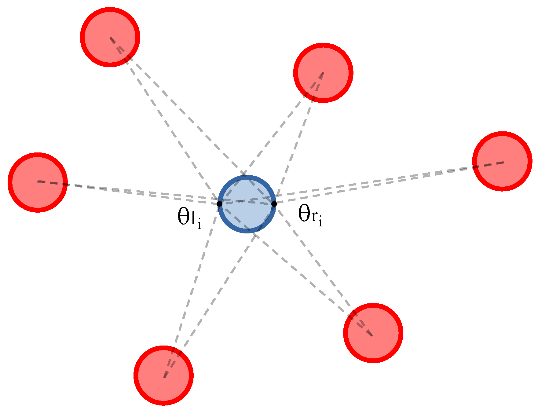
The simulation of the buoyancy forces is accomplished by the model proposed by Ogami [7], where the vorticity generated from heat is represented by a modification of the strength of each vortex blob during the simulation. Mathematically, this effect is simulated as a direct interpretation of the buoyancy term in Equation (1). Therefore, for the i-th discrete vortex element, the change in strength is given as follows:

$$\delta {\Gamma }_i=Ri{\displaystyle \frac{\partial \theta }{\partial x_1}}\Delta t\Delta A_i,$$

(29)

where $\Delta A_i=\pi {\sigma }_{V_i}^2$ is the area of the i-th vortex element. The derivative in the right hand side of Equation (29) is solved by a centered difference method truncated on the first term:

$${\left.{\displaystyle \frac{\partial \theta }{\partial x_1}}\right|}_i={\displaystyle \frac{{\theta }_{r_i}-{\theta }_{l_i}}{2{\sigma }_{V_i}}},$$

(30)

where ${\theta }_r$ and ${\theta }_l$ are the temperatures on the right- and left-most points of the i-th vortex blob. This problem also needs a number of operations proportional to the square of the number of particles. The method can be visually represented by Figure 2.

3. Results and Discussion

An initial validation of the numerical method was conducted by comparing the numerical solutions of the surface representation method (the Panels Method) for the diffusion and advection problems with the analytical results.

The first validation consists of representing a cylinder of radius $r_0$ in two dimensions (a circle) by $MB$ uniform source flat panels with constant length, subjecting it to an incident flow. This problem is well-known in fluid dynamics and can be represented using the potential theory as an incident flow superposed to a dipole [27]. Using the complex potential function, the velocity components (u and v) at each point $z=x+iy$ of the complex plane can be written as follows:

$$W\left(z\right)=u-iv=1-{\displaystyle \frac{r_0^2}{z^2}}$$

(31)

By discretizing the cylinder in $MB=300$ panels, the graphic comparison between Equation (31) and the Panels Method is shown in Figure 3.

Figure 3 shows that the Panels Method converges to the potential solution, with $MB=300$ source flat panels discretizing the body. The mean absolute error in each velocity component was about $0.5\%$. This order of error allows the body to be appropriately represented in the numerical solution. However, given the potential nature of the Panels Method, it is necessary to implement a diffusion algorithm, which will be paired with an advection scheme, to simulate the flow.

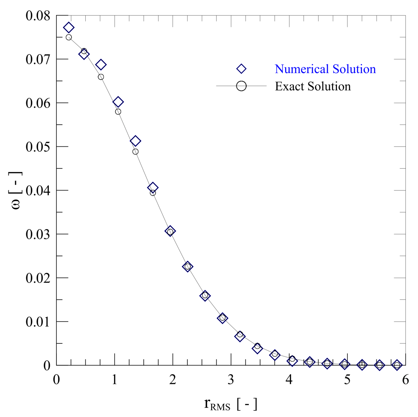
The verification of the diffusion method is made by distributing Z $=6000$ vortex blobs at the origin of a polar plane, each with strength $1/6000$. The fluid is assumed to have a unitary kinematic viscosity coefficient. Then, the particles are allowed to diffuse in 20 time steps of $\Delta t=0.05$ via Random Walk Method [5]. After the last time step, the polar plane is divided into 20 radial strips ranging from $r=0$ to $r=6$. At each annular region, the root main square (RMS) radius is calculated, and this is the value where the vorticity distribution is considered to be concentrated for graphical representation. If n vortex blobs are inside an annular region, the vorticity value is then obtained as follows:

$${\omega }_{r-(r+\Delta r)}={\displaystyle \frac{n}{Z\pi [{(r+\Delta r)}^2-r^2]}}$$

(32)

Then, Equation (32) is compared with the analytical distribution:

$$\omega (r,t)={\displaystyle \frac{1}{\pi \left(4\nu t\right)}}exp\left(-{\displaystyle \frac{r^2}{4\nu t}}\right)$$

(33)

Using the previous values, the distribution can be seen in Figure 4.

The average relative error at each data point is $7.3\%$, which is considered acceptable for the number of vortex elements used. In a larger simulation, the error tends to be lower since the number of elements is higher, which is beneficial for the Random Walk Method.

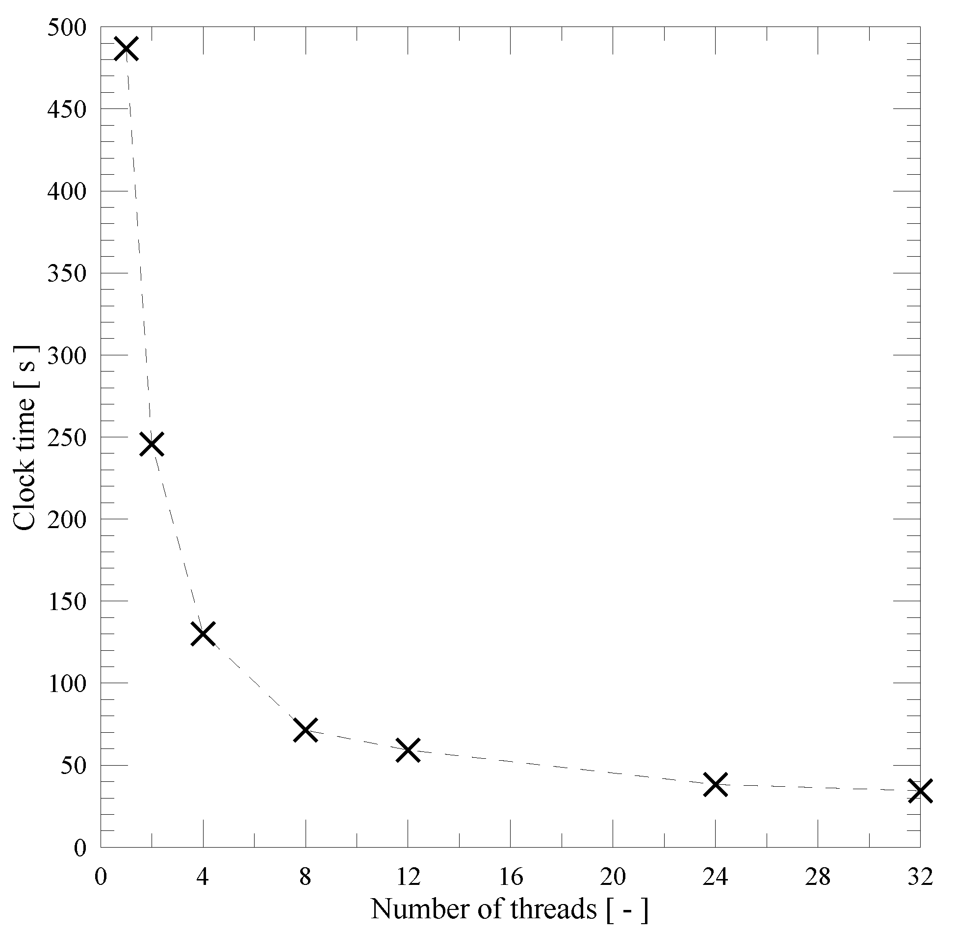
Considering that the vortex–temperature interactions are computationally expensive, consisting of three kinds of operations, each with a complexity of $\mathcal{O}\left(N^2\right)$ for N particles, this paper opted to use an OpenMP implementation in the numerical code to accelerate such interactions. Figure 5 shows the wall clock time needed to simulate only the three vortex–temperature interactions for N = 300,000 vortex blobs and 300,000 temperature particles, with increasingly more threads. The particles were randomly distributed inside a rectangle of unitary side length for this test. A speedup of 14.15 times was obtained when comparing the 32 threads implementation with the serial approach (1 thread), with the diminishing returns becoming smaller when using 24–32 threads. This acceleration allows for the simulation of simultaneous vortex–temperature interactions while keeping the number of panels used to discretize the solid surface. All simulations were executed using 32 threads, a processor Intel Core i9-13900KF 3.0 GHz with 32 threads, and a cache of 32 MB. The parallel simulations showed the same numerical precision as the serial version.

Since the initial validation of the numerical code is complete, it is now possible to present the test cases for the flow past a heated circular cylinder.

Table 1. Dimensionless input data used in the simulation.

Description	Value
Diameter (D)	1.0
Inlet flow velocity ($U_{\infty }$)	1.0
Reynolds number (Re)	$1.0\times {10}^5$
Prandtl number (Pr)	0.71
Richardson number (Ri)	0.168 and 0.336
Initial core radius (${\sigma }_V$ and ${\sigma }_T$)	0.001
Time step ($\Delta t$)	0.05
Number of time steps	800
Number of panels (MB)	300
Turbulent Prandtl number ($P{r}_T$)	0.95

shows the non-dimensional parameters adopted as input values in the simulation, and

Table 2. Configuration and results of each test case.

Case	$\mathit{\epsilon }/\mathit{D}$	$\mathit{Ri}$	${\mathit{C}}_{\mathit{D}}$	${\mathit{C}}_{\mathit{L}}$	${\mathit{\theta }}_{\mathit{sep}}$	$\mathit{St}$
#1 *	0.0	0.0	1.223	—	81.0	—
#2	0.0	0.168	1.212	−0.041	82.0°	0.208
#3	0.001	0.168	1.268	−0.093	82.5°	0.202
#4	0.004	0.168	1.277	−0.051	83.5°	0.198
#5	0.007	0.168	1.368	−0.095	82.5°	0.204
#6	0.001	0.336	1.222	−0.047	82.0°	0.208

* Values for case #1 were obtained from [33] using the Discrete Vortex Method from our group formulation.

shows the mean values for drag and lift coefficients obtained through the simulations, as well as the separation point and Strouhal number. It can be seen that the drag coefficient increases with higher values of surface roughness.

Test case #1 is a benchmark simulation without surface roughness effects and heat transfer from [33], using the same method but only considering the vortex wake, whereas the experimental results from [34] are $C_D=1.{20}^{\pm 10\%}$ and $St=0.{19}^{\pm 10\%}$. When considering mixed convection (case #2), a reduction in drag followed by an increase in the separation angle, ${\theta }_{sep}$, is observed, showing how the mixed convection interacts with the smooth cylinder.

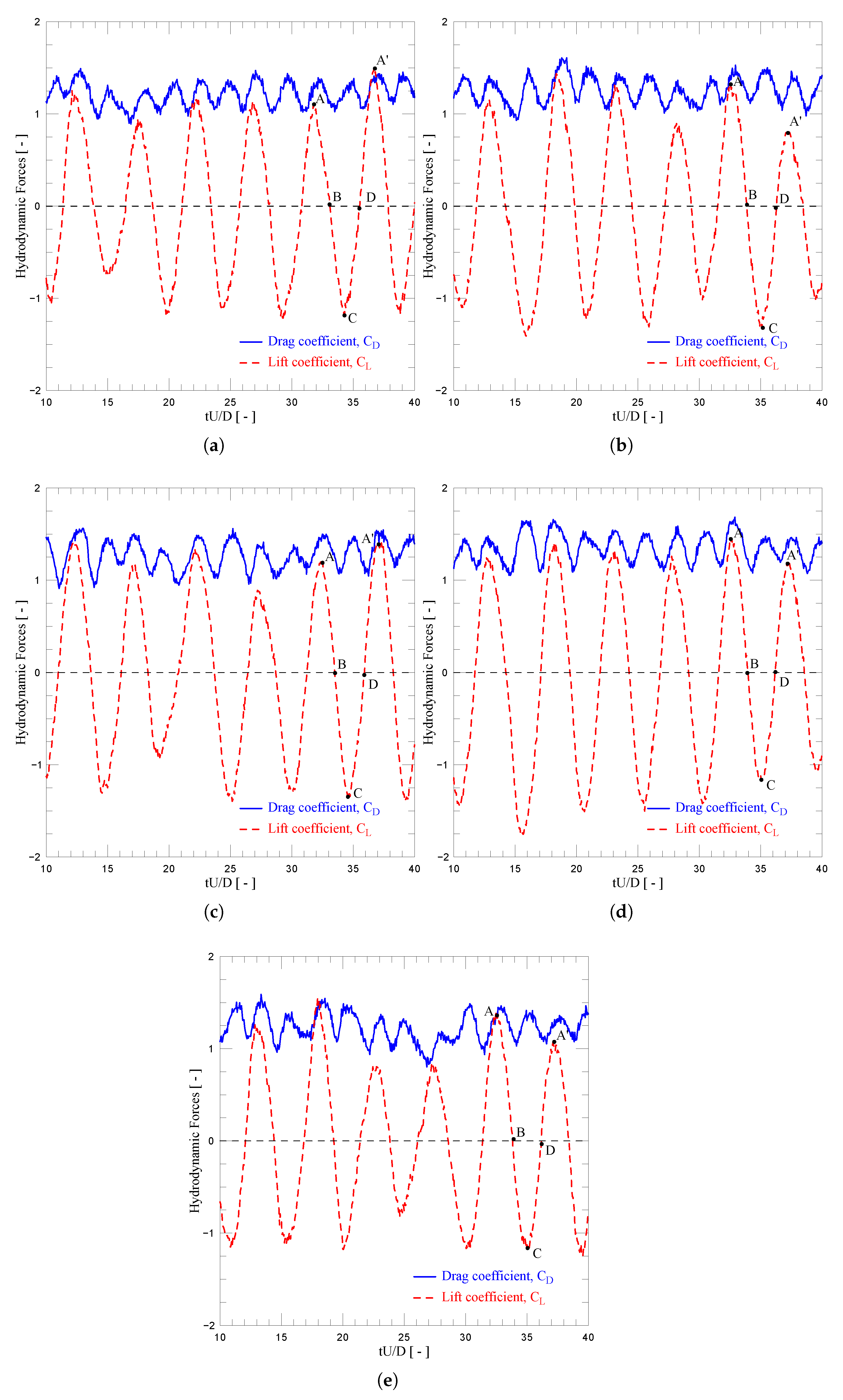
Figure 4 shows the transient drag and lift coefficients in every simulation. Im test cases #2 and #3, the main difference was due to the effects of surface roughness, which increases in test cases #4 and #5. This effect can be observed in the increase in the amplitude of the drag curve as $\epsilon /D$ increases from 0.0 to 0.007. This is caused by the influence of the surface roughness in the boundary layer flow, which leads to an increase in the drag forces of approximately 12.9%. In the present simulations, an early transition s not observed and/or drag crisis is noted in in [17,33]. This happens due to the combined effects of a rough surface and mixed heat transfer, indicating that the temperature field interacts with the vorticity field avoiding the drag crisis occurrence in the studied cases.

However, when considering $Ri=0.336$ in Figure 6e, it can be observed that the behavior of the drag and lift curves changed when compared to the previous cases in the interval between tU/D = 20 and 30. This happens due to the interaction of the first pair of counter-rotating vortices in the near wake. The average drag coefficient in this scenario, with more intense buoyancy forces, is reduced by approximately 3.6% when compared to test case #3. Therefore, the proposed description of this kind of turbulent flow, using a Lagrangian approach, can capture the drag reduction using this mixed convection technique.

The average pressure coefficient at each discrete angular position of the cylinder (being zero the frontal stagnation point in the origin and ${180}^{\circ }$ the stagnation point at (1.0, 0.0) measured in a clockwise manner) is shown in Figure 7 for the five test cases. Overall, Figure 7 shows that higher roughness value tends to increase the base pressure, with simulation #5 being the exception with the lowest base pressure. This value also has the largest deviation from the others as the angular position increases, suggesting that this roughness value impacts the vortex formation in different ways than the previous cases at the same Richardson number. Meanwhile, test case #6 at a higher Richardson number captured a reduction in the drag coefficient, which can be seen by its pressure coefficient consistently above the other test cases. The deviation from the lowest pressure near ${70}^{\circ }$ to the experimental results [34] can be attributed to the constant length of each panel used to discretize the surface, and a finer distribution at this region could better capture the pressure gradient.

If one compares the wakes at the last time step for test cases #2 and #5, the surface roughness effects in the vortex dynamics become more apparent (Figure 8). Test case #5 changes the wake more strongly, causing a larger region of lower velocities in the rear part of the cylinder.

When comparing the influence of the Richardson number effects, the wake is affected in a significant way. Test case #3 had a Strouhal number of 0.202, while test case #6 presented a Strouhal number of 0.208, showing that the frequency of the shedding was close in both cases; however, a qualitative view of each wake shows an expressive change (see Figure 9). The Richardson number of 0.336 causes the spacing among the initial structures to increase, and the shapes become stretched, deforming the structure in the direction of the gravitational acceleration. The separation angle did not change in an expressive way, as can be seen in Table 2, indicating that the buoyancy forces are determinant in the drag reduction in this situation.

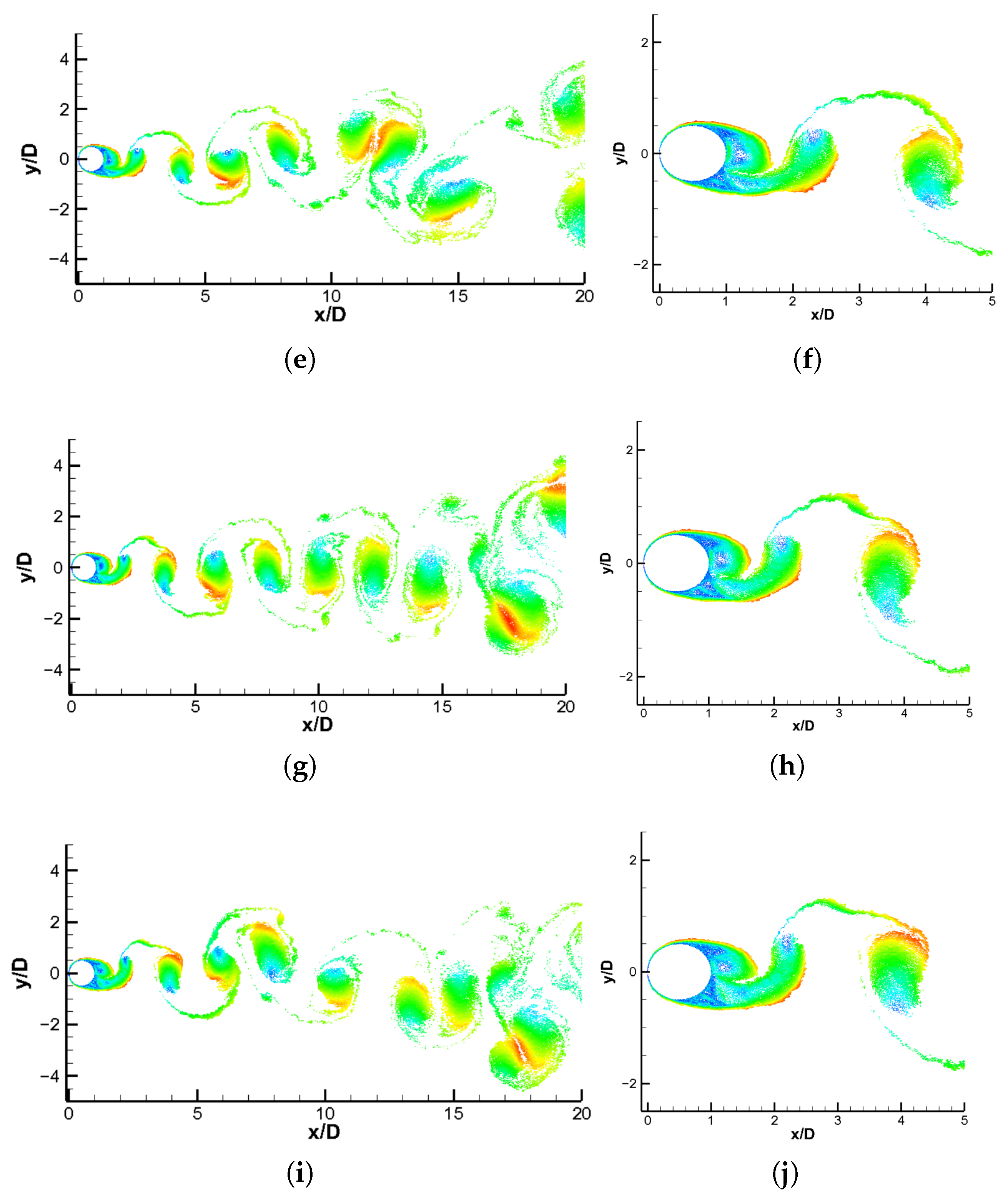
A broader comparison can be made by inspecting the vortex wake near the end of all simulations, which is shown in Figure 10. In this comparison, it can be seen that the roughness effects cause the wake and the vortex sheets to deform more as $\epsilon /D$ increases. Additionally, for test case #5, the highest surface roughness simulated, the velocity field is characterized by more areas, with a higher magnitude in the far wake, and those intense vortical structures affect the sheets, making them less visible as the vorticity disperses at higher $x/D$ values.

The wake of point A′ is shown in Figure 10 for test cases #2 to #6 to aid in the physical interpretation of what happens to the flow due to the combined effects of roughness surface and natural convection in the simulations. Figure 10a shows lower velocities in the near wake, particularly in the boundary layer detachment region, while the other test cases have higher velocities in the near wake due to the roughness effects. This higher velocity, in addition to the recirculating region that forms the clockwise vortex, which will be released into the domain, results in lower pressure at the top of the cylinder and an increasing drag coefficient at this instant (as shown in Figure 6; the maximum lift peak is close to the maximum drag coefficient). When comparing Figure 10a–h with Figure 10i,j, it can be observed that at this time step, the near wake has a slight dislocation in the positive direction of the y-axis. Thus, the near wake becomes thinner in case #6, which explains the smaller drag coefficient that was observed in Table 2. This displacement is due to the increased effects of the buoyancy forces at the near wake, represented by a Richardson number of 0.336.

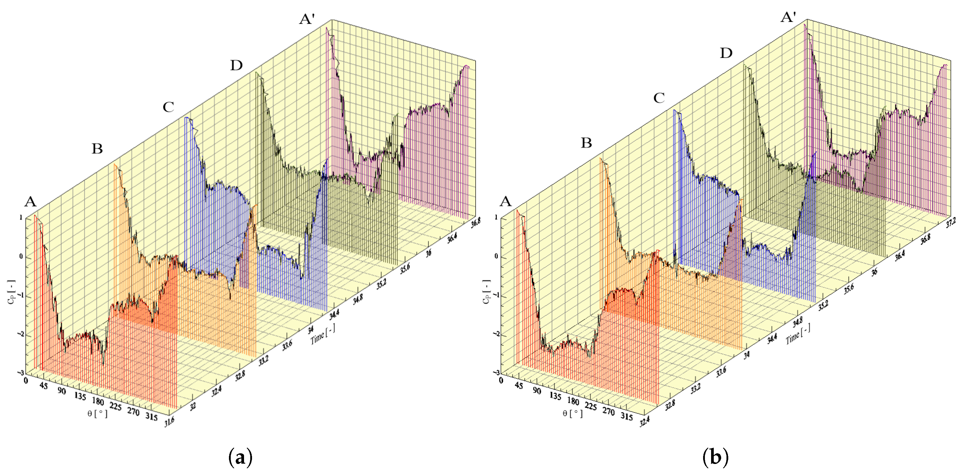
Focusing once more on the pressure coefficient, the effects of roughness and the Richardson number can be compared, analyzing the distribution of $C_p$ at points of interest (A, B, C, D, and A^′) to investigate the Gerrard mechanism [35]. Point A represents the instant when a clockwise vortex sheds from the top of the cylinder (also the maximum lift coefficient value). Point B is the instant at which this vortex is incorporated in the wake (and when the lift coefficient changes its signal). Point C denotes the shedding of a counter clockwise vortex (minimum lift coefficient), and point D is where this counterclockwise vortex joins the wake (lift coefficient changes signal). The comparison between cases #2 and #5 is shown in Figure 11.

Figure 11 shows how the pressure coefficient behaves at every point of interest. It can be seen that point A of test case #2 has a higher pressure coefficient at the rear part of the cylinder (around $\theta ={180}^{\circ }$) than the one observed in case #5. The peak after ${225}^{\circ }$ for test case #5 has a higher value than the value obtained in case #2. This results in the higher drag coefficient for case #5 and explains how the higher roughness surface affected the distribution of the pressure coefficient. Moreover, it can be seen that in the instant represented by point A, a clockwise vortex structure is shedding from the upper surface of the cylinder due to the lower pressure coefficient in this region, resulting in the maximum lift coefficient at this instant (see Figure 6a,d). At point B, when the lift coefficient changes its signal, an equilibrium of the forces can be seen on the upper and lower half of the cylinder, indicating that the initial clockwise structure has entered the flow, and the counterclockwise vortex starts gaining circulation. This vortex keeps gaining circulation until it is ready to shed at point C in the lower half of the cylinder. When it sheds, the alternating mechanism starts feeding the upper half with circulation, and the point where the forces are once again in balance is seen in point D. Point A′ is physically the same as point A but after a period of the oscillation.

4. Conclusions

In this work, the Temperature Particles Method (TPM) is implemented for a two-dimensional turbulent flow around a cylinder with a circular cross section. The computational code used a two-dimensional LES type turbulence model to calculate the eddy viscosity and turbulent thermal diffusivity for the vortex cloud and temperature cloud. The innovation proposed concerns a model to consider the surface roughness influence on the thermal boundary layer without changing the surface geometry, adapting a previously validated implementation for the hydrodynamic boundary layer. The values of $C_D$, $C_L$, $C_p$, and $St$ for selected cases were compared, as well as the wakes for points of interest.

The temperature roughness model affected the flow slightly. The increase in the Richardson number resulted in a reduction in the drag coefficient, while higher surface roughness values increased the drag coefficient. This last result does not predict a transition of the turbulent regime after the critical region—perhaps due to the combined effects of surface roughness and mixed convection.

Further studies will be conducted to assess the sensitivity of the method for other values of the Richardson number, but the results presented here are promising. The authors will continue the development of their in-house code with the aim of simulating other practical engineering problems.

References

1. Rashidi, S.; Hayatdavoodi, M.; Esfahani, J.A. Vortex shedding suppression and wake control: A review. Ocean Eng. 2016, 126, 57–80. [Google Scholar] [CrossRef]
2. Al-Rubaiy, A. The Effect of Surface Roughness and Free Stream Turbulence on the Flow and Heat Transfer around a CircularCylinders. Ph.D. Thesis, The University of Sheffield, Sheffield, UK, 2018. [Google Scholar]
3. Dwivedi, A.R.; Dhiman, A.K. Flow and heat transfer analysis around tandem cylinders: Critical gap ratio and thermal cross-buoyancy. J. Braz. Soc. Mech. Sci. Eng. 2019, 41, 487. [Google Scholar] [CrossRef]
4. Afgan, I.; Kahil, Y.; Benhamadouche, S.; Ali, M.; Alkaabi, A.; Sofiane Berrouk, A.; Sagaut, P. Cross flow over two heated cylinders in tandem arrangements at subcritical Reynolds number using large eddy simulations. Int. J. Heat Fluid Flow 2023, 100, 109115. [Google Scholar] [CrossRef]
5. Chorin, A. Numerical Study of Slightly Viscous Flow. J. Fluid Mech. 1973, 57, 785–796. [Google Scholar] [CrossRef]
6. Smith, P.A.; Stansby, P.K. An efficient surface algorithm for random-particle simulation of vorticity and heat transport. J. Comput. Phys. 1988, 81, 349–371. [Google Scholar] [CrossRef]
7. Ogami, Y. Simulation of heat-fluid motion by the vortex method. JSME Int. J. 2001, 44, 513–519. [Google Scholar] [CrossRef]
8. Leonard, A. Vortex methods for flow simulation. J. Comput. Phys. 1980, 37, 289–335. [Google Scholar] [CrossRef]
9. Degond, P.; Mas-Gallic, S. The weighted particle method for convection-diffusion equations. Part 1. The case of an isotropic viscosity. Math. Comput. 1989, 53, 485–507. [Google Scholar] [CrossRef]
10. Degond, P.; Mas-Gallic, S. The weighted particle method for convection-diffusion equations. Part 2. The anisotropic case. Math. Comput. 1989, 53, 509–525. [Google Scholar] [CrossRef]
11. Fishelov, D. A new vortex scheme for viscous flows. J. Comput. Phys. 1990, 86, 211–224. [Google Scholar] [CrossRef]
12. Ogami, Y.; Akamatsu, T. Viscous flow simulation using the discrete vortex model—The diffusion velocity method. Comput. Fluids 1991, 19, 433–441. [Google Scholar] [CrossRef]
13. Shankar, S.; van Dommelen, L. A new diffusion procedure for vortex methods. J. Comput. Phys. 1996, 127, 88–109. [Google Scholar] [CrossRef]
14. Rossi, L. Resurrecting Core Spreading Vortex Methods: A New Scheme that is Both Deterministic and Convergent. Siam J. Sci. Comput. 1996, 17, 370–397. [Google Scholar] [CrossRef]
15. Beale, J.T.; Majda, A. Rates of convergence for viscous splitting of the Navier-Stokes equations. Math. Comput. 1981, 37, 243–259. [Google Scholar] [CrossRef]
16. Torres, C.; Barba, L. Fast radial basis function interpolation with Gaussians by localization and iteration. J. Comput. Phys. 2009, 228, 4976–4999. [Google Scholar] [CrossRef]
17. Bimbato, A.; Alcântara Pereira, L.; Hirata, M. Development of a new Lagrangian vortex method for evaluating effects of surfaces roughness. Eur. J. Mech.-B/Fluids 2019, 74, 291–301. [Google Scholar] [CrossRef]
18. Alcântara Pereira, L.; Hirata, M.; Silveira Neto, A. Vortex Method with Turbulence Sub-Grid Scale Modelling. J. Braz. Soc. Mech. Sci. Eng. 2003, 25, 140–146. [Google Scholar] [CrossRef]
19. Prendergast, J.M. Simulation of Unsteady 2-D Wind by a Vortex Method. Ph.D. Thesis, Department of Engineering, University of Cambridge, Cambridge, UK, 2007. [Google Scholar]
20. Rasmussen, J.T.; Hejlesen, M.M.; Larsen, A.; Walther, J.H. Discrete vortex method simulations of the aerodynamic admittance in bridge aerodynamics. J. Wind. Eng. Ind. Aerodyn. 2010, 98, 754–766. [Google Scholar] [CrossRef]
21. Chiaradia, T.R.; Carvalho, G.F.M.; Bimbato, A.M.; Alcântara Pereira, L.A. A Contribution to the Temperature Particles Method—Implementation of a Large-Eddy Simulation (LES) Model for the Temperature Field. Appl. Sci. 2025, 15, 4122. [Google Scholar] [CrossRef]
22. Achenbach, E.; Heinecke, E. On vortex shedding from smooth and rough cylinders in the range of Reynolds numbers 6000 to 5,000,000. J. Fluid Mech. 1981, 109, 239–251. [Google Scholar] [CrossRef]
23. Tian, X.; Li, D.; Liu, G.; Xie, Y.; Deng, W.; Xie, D. Experimental study on the hydrodynamic characteristics of cylinder with rough surface. J. Mar. Sci. Technol. 2019, 25, 842–848. [Google Scholar] [CrossRef]
24. Marty, A.; Schoefs, F.; Soulard, T.; Berhault, C.; Facq, J.V.; Gaurier, B.; Germain, G. Effect of Roughness of Mussels on Cylinder Forces from a Realistic Shape Modelling. J. Mar. Sci. Eng. 2021, 9, 598. [Google Scholar] [CrossRef]
25. Sun, C.; Zhou, T.; An, H.; Zhu, H.; Cheng, L. Experimental studies on wake structures of a circular cylinder with different surface roughness heights. Int. J. Heat Fluid Flow 2022, 94, 108941. [Google Scholar] [CrossRef]
26. Moraes, P.G.d.; Oliveira, M.A.d.; Bimbato, A.M.; Alcântara Pereira, L.A. A Lagrangian Description of Buoyancy Effects on Aircraft Wake Vortices from Wing Tips near a Heated Ground Plane. Energies 2022, 15, 6995. [Google Scholar] [CrossRef]
27. Katz, J.; Plotkin, A. Low Speed Aerodynamics: From Wing Theory to Panel Methods; McGraw Hill: New York, NY, USA, 1991. [Google Scholar]
28. Métais, O.; Lesieur, M. Spectral large-eddy simulation of isotropic and stably stratified turbulence. J. Fluid Mech. 1992, 239, 157–194. [Google Scholar] [CrossRef]
29. Tritton, D.J. Physical Fluid Dynamics; Van Nostrand Reinhold Co.: New York, NY, USA, 1977. [Google Scholar]
30. Shintani, M.; Akamatsu, T. Investigation of Two Dimensional Discrete Vortex Method with Viscous Diffusion Model. Comput. Fluid Dyn. J. 1994, 3, 237–254. [Google Scholar] [CrossRef]
31. Ferziger, J.H. Numerical Methods for Engineering Application; John Wiley & Sons, Inc.: Hoboken, NJ, USA, 1981. [Google Scholar]
32. Guimarães de Moraes, P.; Oliveira, M.A.; Andrade, C.; Bimbato, A.; Alcântara Pereira, L. Effects of surface roughness and wall confinement on bluff body aerodynamics at large-gap regime. J. Braz. Soc. Mech. Sci. Eng. 2021, 43, 397. [Google Scholar] [CrossRef]
33. Bimbato, A.M.; Alcântara, Pereira, L.A.; Hirata, M.H. Study of Surface Roughness Effect on a Bluff Body—The Formation of Asymmetric Separation Bubbles. Energies 2020, 13, 6094. [Google Scholar] [CrossRef]
34. Blevins, R.D. Applied Fluid Dynamics Handbook; Van Nostrand Reinhold Co.: New York, NY, USA, 1984. [Google Scholar]
35. Gerrard, J.H. The mechanics of the formation region of vortices behind bluff bodies. J. Fluid Mech. 1966, 25, 401–413. [Google Scholar] [CrossRef]
Figure 1. Representation of the geometry of the chosen problem.
Fluids 10 00288 g001
Figure 2. Schematic representation of the location at which each discrete vortex blob (in blue) receives the temperature inductions from the temperature blobs (in red).
Fluids 10 00288 g002
Figure 3. Comparison between velocity components predicted by the potential theory and the Panels Method: (a) velocity component u; (b) velocity component v.
Fluids 10 00288 g003
Figure 4. Numerical solution of the radial vorticity distribution compared to the analytical solution.
Fluids 10 00288 g004
Figure 5. Comparison of the time needed to complete the vortex–temperature interactions for 300,000 of each particle (vortex blobs and temperature particles).
Fluids 10 00288 g005
Figure 6. Temporal variations of drag and lift coefficients during the numerical simulation: (a) ε / D = 0.0 ; R i = 0.168 ; (b) ε / D = 0.001 ; R i = 0.168 ; (c) ε / D = 0.004 ; R i = 0.168 ; (d) ε / D = 0.007 ; R i = 0.168 ; (e) ε / D = 0.001 ; R i = 0.336 .
Fluids 10 00288 g006
Figure 7. Pressure coefficient distribution of each test case compared to the experimental data.
Fluids 10 00288 g007
Figure 8. Vortex wake at the end of the simulation: (a) test case #2 (Ri = 0.168, ε / d = 0.0 ); (b) test case #5 (Ri = 0.168, ε / D = 0.007 ) .
Fluids 10 00288 g008
Figure 9. Temperature clouds at the end of the simulation: (a) test case #3 (Ri = 0.168, ε / D = 0.001 ); (b) test case #6 (Ri = 0.336, ε / D = 0.001 ) .
Fluids 10 00288 g009
Figure 10. Full and near vortex wakes corresponding to the instants of time represented by points A′ marked in Figure 6 for th test cases: (a) Full wake— ε / D = 0.0 ; R i = 0.168 ; (b) Near wake— ε / D = 0.0 ; R i = 0.168 ; (c) Full wake— ε / D = 0.001 ; R i = 0.168 ; (d) Near wake— ε / D = 0.001 ; R i = 0.168 ; (e) Full wake— ε / D = 0.004 ; R i = 0.168 ; (f) Near wake— ε / D = 0.004 ; R i = 0.168 ; (g) Full wake— ε / D = 0.007 ; R i = 0.168 ; (h) Near wake— ε / D = 0.007 ; R i = 0.168 ; (i) Full wake— ε / D = 0.001 ; R i = 0.336 ; (j) Near wake— ε / D = 0.001 ; R i = 0.336 .
Fluids 10 00288 g010aFluids 10 00288 g010b
Figure 11. Pressure coefficients at points A—A′: (a) ε / D = 0.0 ; R i = 0.168 ; (b) ε / D = 0.007 ; R i = 0.168 .
Fluids 10 00288 g011