Abstract
Ensuring the structural integrity of mechanical components operating in fluid environments requires precise and reliable monitoring techniques. This study presents a methodology for reconstructing the full-field deformation of a flexible aluminium plate subjected to unsteady water flow in a water tunnel, using a structural modal reconstruction approach informed by experimental data. The experimental setup involves an aluminium lamina (200 mm × 400 mm × 2.5 mm) mounted in a closed-loop water tunnel and exposed to a controlled flow with velocities up to 0.5 m/s, corresponding to Reynolds numbers on the order of , inducing transient deformations captured through an image-based optical tracking technique. The core of the methodology lies in reconstructing the complete deformation field of the structure by combining a reduced number of vibration modes derived from the geometry and boundary conditions of the system. The novelty of the present work consists in the integration of the Internal Strain Potential Energy Criterion (ISPEC) for mode selection with a data-driven machine learning framework, enabling real-time identification of active modal contributions from sparse experimental measurements. This approach allows for an accurate estimation of the dynamic response while significantly reducing the required sensor data and computational effort. The experimental validation demonstrates strong agreement between reconstructed and measured deflections, with normalised errors below 15% and correlation coefficients exceeding 0.94, confirming the reliability of the reconstruction. The results confirm that, even under complex, time-varying fluid–structure interactions, it is possible to achieve accurate and robust deformation reconstruction with minimal computational cost. This integrated methodology provides a reliable and efficient basis for structural health monitoring of flexible components in hydraulic and marine environments, bridging the gap between sparse measurement data and full-field dynamic characterisation.
1. Introduction
Modal superposition is a well-established method in structural dynamics, based on the linear combination of modal shapes to describe displacements or strains. It has been widely used in engineering for decades, primarily because it offers considerable savings in time and computational resources compared to direct numerical integration methods [1]. Its most common application is in the evaluation of the transient dynamic response of structures [2], but it has also found widespread use in other domains, such as in the study of the response of seismic sites [3,4,5].
Beyond these classical applications, modal superposition plays a central role in modal reconstruction, i.e., the reconstruction of a structure’s deformation field from sparse measurement data. Modal reconstruction algorithms provide a theoretical framework for recovering the full displacement field of a structure starting from a limited number of discrete measurements [6,7]. The underlying assumption is that the structural response to dynamic loading can be accurately represented by a reduced set of vibration modes, thus enabling efficient analysis while significantly reducing the amount of required measurement data. In engineering practice, this approach is particularly useful for objects that are isotropic, homogeneous, and linearly elastic, since displacement and strain measurements can then be related to stresses by compatibility conditions and Hooke’s law. In such contexts, reconstructing the displacement and strain fields also enables inference of the stress state of the entire structure, which is of high relevance for monitoring machines and critical safety systems.
Modal reconstruction has also been explored to reconstruct the shape from partial measurements [8,9]. In these applications, the deformation of an object can be inferred from limited displacement or strain signals, offering a powerful tool for practical engineering problems. This is particularly relevant in structural health monitoring (SHM), where displacements and strains often need to be estimated in real time from sparse measurements taken in accessible locations that do not compromise system operation [10,11]. If modal shapes are available from a finite element (FE) model, the measured displacements at these few points can be used to determine the modal coordinates, which quantify the contribution of each vibration mode to the overall deformation. These coordinates then form the basis for reconstructing the full-field structural response, offering valuable information for damage detection and anomaly identification.
A fundamental challenge in modal reconstruction is the problem of mode selection [7,12]. For both computational efficiency and accuracy, it is desirable to retain the smallest number of modes that capture the essential features of the dynamic response. However, the selection cannot be arbitrary: only the modes that significantly contribute to the deformation under the given loading conditions should be retained. Over the years, several selection criteria have been proposed [13,14,15,16]. Among these, the most relevant for the present study is the Internal Strain Potential Energy Criterion (ISPEC) [17].
The ISPEC is based on quantifying the reconstruction capability of each vibration mode through its associated internal strain potential energy. This formulation is independent of the full FE solution and can be applied directly from sparse deformation or strain measurements combined with material properties. Unlike other criteria, the ISPEC can operate with measurements from a discrete number of points on the structure without requiring full-field knowledge of the deformation. This makes it particularly attractive for SHM applications, where measurement accessibility is often limited. From a theoretical point of view, the criterion is consistent with the energetic contribution of each mode to the structural deformation, retaining only the modes whose strain energy exceeds a predefined threshold. This ensures both reconstruction accuracy and computational efficiency.
Although the theoretical framework for modal reconstruction and the ISPEC is well established, its integration into SHM opens new opportunities. Real-time reconstruction of displacement fields can be achieved by combining ISPEC-based mode selection with advanced data-driven identification frameworks.
In this work, for the first time, a methodology is proposed that integrates the ISPEC with a machine learning-based classification framework to enable real-time reconstruction of full-field displacements from sparse measurements. Specifically, a random forest classifier is trained on synthetic deformation data generated from a simplified FE model of the monitored structure. The FE model is developed in Ansys APDL and discretised using SOLID185 linear solid elements. These elements are well suited for modelling three-dimensional solid structures, as each element consists of eight nodes with three translational degrees of freedom per node, corresponding to displacements in the global x, y, and z directions [18]. This modelling choice ensures a reliable representation of the structural behaviour while maintaining computational efficiency, which is essential for the generation of a sufficiently large synthetic dataset to be used for training the classifier. The algorithm is then applied to sparse experimental measurements, reconstructing the displacement field and validating predictions against independent reference points. Experimental data were obtained by placing an aluminium flat plate in an unstable flow generated by a custom-designed water tunnel. The characteristics of the incoming flow were measured using a planar PIV system. The same PIV camera was also used to record the displacement of the plate.
2. Experimental Setup
2.1. Water Tunnel Description
The experiments were conducted in the low-speed water tunnel located at the University of Tuscia. The facility is a closed-loop water tunnel featuring a test section with dimensions . The water flow is provided by a Caprari pump driven by a 4 kW asynchronous electric motor. The flow rate is controlled using a series of bypass valves and flow velocity can be varied from up to , enabling the achievement of Reynolds numbers on the order of with a stable and quite clean flow rate. Details about the experimental facility are reported in Figure 1.
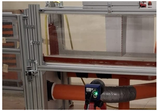
Figure 1.
General overview showing the water tunnel, the lamina, and the high-resolution camera.
The facility was equipped with a planar Particle Image Velocimetry (PIV) system provided by LaVision. The system includes a CMOS camera with a sensor resolution of pixels resolving 123 fps at full resolution. The camera was equipped with Nikkor AF-S 58mm f/1.4G lenses by Nikon (Melville, NY, USA). Water was seeded by hollow glass spheres, with a nominal diameter of 10 m and specific weight of 1.05 . The illumination of the field of view is provided by an LED light source capable of producing 1350 lumens, producing a collimated light sheet wide and thick. Camera calibration, acquisition, and post-processing are supported by LaVision Davis 11 software. The statistical analysis was performed over a population of 200 images.
2.2. Setup Definition
The test specimen used in the experimental campaign is a flexible aluminium lamina with dimensions (width × height × thickness). The plate is vertically mounted inside the test section of the water tunnel, with its longer edge (400 mm) oriented vertically and partially immersed in water. The upper portion remains above the free surface and is fully accessible to optical measurements.
The top edge of the lamina is clamped using a rigid vice, ensuring a fixed–free boundary condition. The water level is adjusted so that only the lower section is submerged, while the upper, emerged portion is monitored through the camera. This is positioned laterally to the tunnel and captures the lamina’s out-of-plane deformation induced by the fluid flow.
To track displacements, a sequence of high-contrast reflective tape markers is applied along the vertical midline of the section of the lamina. These markers are made of retroreflective tape and are equally spaced at intervals, starting from the clamped edge and extending downward. The number of markers visible depends on the water level and camera framing, as only those located above the free surface are acquired by the optical system.
Among the visible markers, the first seven from the clamped end are used as input for the SHM algorithm. These provide the minimum spatial information necessary to initialise the modal reconstruction framework. Any additional visible markers positioned further from the clamp are excluded from the input phase and instead used for validation purposes by comparing experimental and reconstructed displacements.
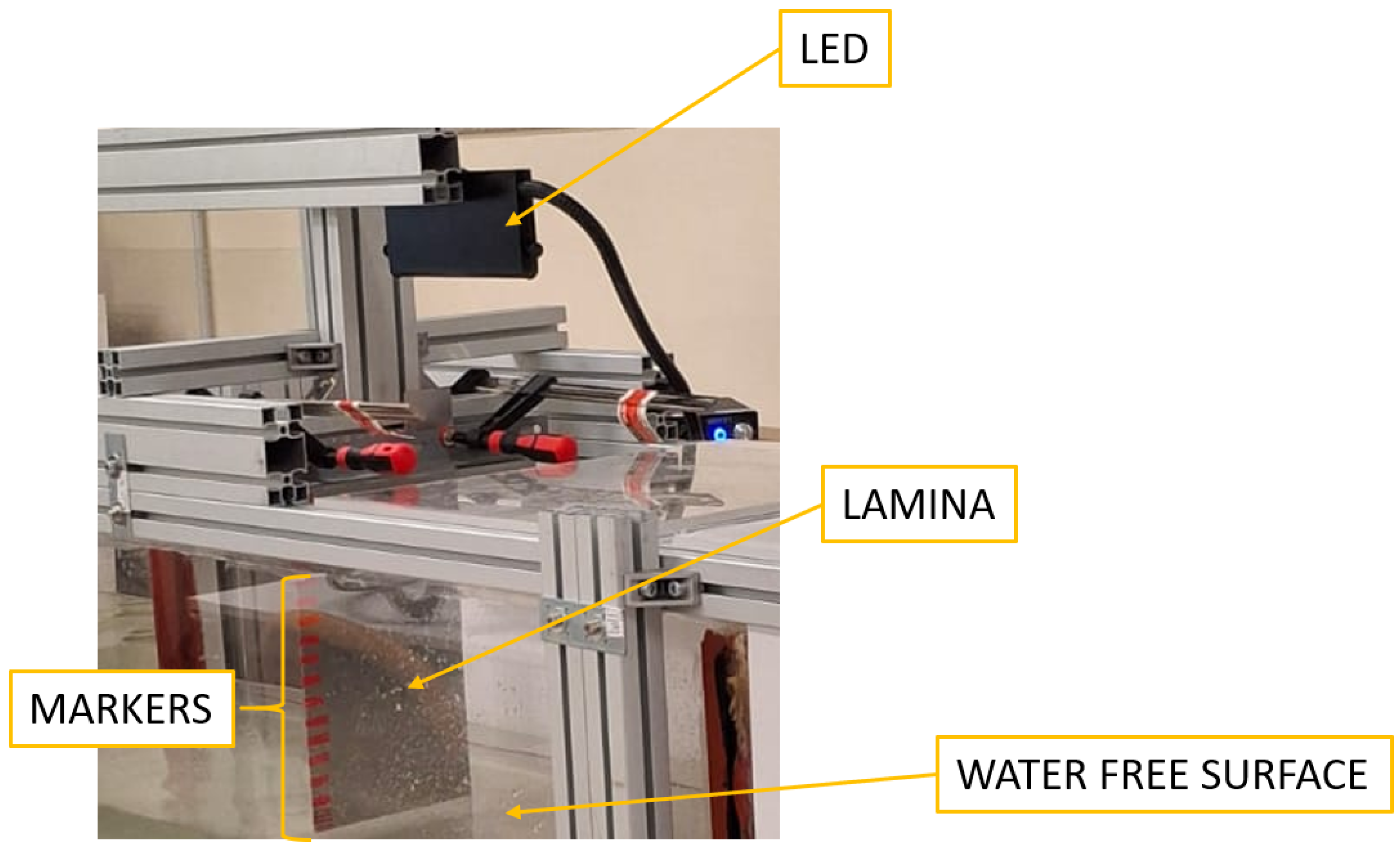
A photograph of the experimental setup, showing the aluminium lamina and its clamping system, is provided in Figure 2. The distribution and roles of the markers are schematically illustrated in Figure 3.
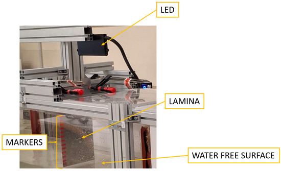
Figure 2.
Detailed view with labelled arrows indicating the positions of the various components.
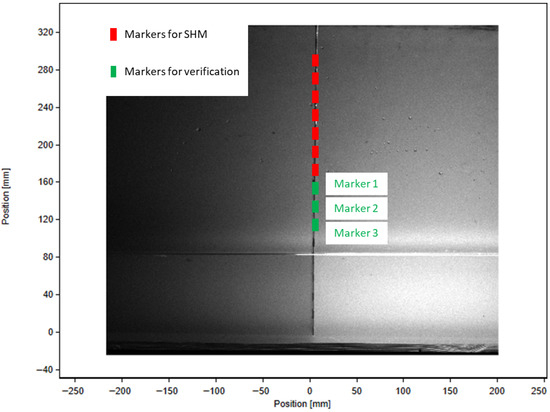
Figure 3.
Marker layout as captured by the camera and visualised using LaVision software.
3. Methodology
3.1. Measurement Selection and Data Usage
The proposed methodology reconstructs the full deformation field of a flexible aluminium plate using sparse displacement measurements, acquired experimentally through image-based tracking techniques. To ensure consistent spatial sampling, ten equidistant markers were tracked along the longitudinal axis of the plate. Only the first seven markers, those located nearest to the clamped boundary, are used as input for the reconstruction algorithm. The remaining three markers, located closer to the water free surface, are excluded from the modal reconstruction process and instead serve as reference points to validate the accuracy of the predicted displacement field.
3.2. Displacement Measurement via Computer Vision Tracking
Displacement measurements were obtained through a custom Python (3.10 version) script implementing a computer vision tracking routine based on the OpenCV library. The method employs the TrackerCSRT algorithm, which is well-suited for accurate localisation of non-rigid targets under partial occlusion and varying illumination.
The procedure begins with the manual selection of rectangular Regions of Interest (ROIs) corresponding to reflective tape markers applied along the longitudinal axis of the plate. For each ROI, the CSRT tracker estimates the marker’s centroid position in pixel coordinates for every frame of the acquired image sequence. The tracking is performed simultaneously for all markers using the MultiTracker framework, ensuring synchronous displacement histories.
Pixel coordinates are converted into physical units (millimetres) using a calibrated scale factor obtained from the experimental setup. For each marker i, the deflection component is calculated by subtracting the initial reference position from the corresponding time-varying tracked position. The resulting displacement time series are stored as NumPy arrays for subsequent use in the modal reconstruction stage.
3.3. Modal Reconstruction Framework
The SHM strategy is based on modal reconstruction, where the structural response is represented as a linear combination of vibration modes derived from the geometry and boundary conditions of the system. Displacement and strain fields are expressed as follows [12,19,20,21,22]:
where and are the displacement and strain vectors, is the vector of modal coordinates, and the matrices and contain the modal displacement and strain shapes, respectively.
Considering an over-determined linear equation system, modal coordinates can be estimated through Langrange multipliers as follows [23]:
It is important to note that, to be valid, the system must be sufficiently determined. Specifically, the number of independent equations, i.e., the product of the number of measurement points and the number of degrees of freedom, must be greater than or equal to the number of retained modes [23]. This condition ensures that the least-squares inversion used to compute is mathematically well-posed and does not lead to overfitting or instability in the reconstruction.
3.4. Strain Potential Energy-Based Mode Selection
To achieve accurate yet efficient reconstruction, only the most significant modes are retained. An energy-based criterion is employed to quantify the contribution of each mode to the strain energy of the system, known as the Internal Strain Potential Energy Criterion (ISPEC) [17,24]. The internal strain energy of a given deformation is defined as follows:
with denoting the elasticity matrix, incorporating material properties such as Young’s modulus and Poisson’s ratio [25,26].
When using modal superposition, the reconstructed strain energy becomes
and the contribution of each individual mode is given by
A non-dimensional metric, the reconstruction capability, is defined as follows:
where is the total strain energy of the actual deformation field. Only modes satisfying the following criterion are retained:
where is a user-defined threshold. This ensures that the reduced basis contains only the most physically relevant modal contributions, improving both numerical stability and interpretability.
3.5. Modal Identification via Machine Learning
Once the most informative modes are selected, they are used to train a machine learning model capable of predicting modal participation based on sparse displacement data.
A random forest classifier, implemented in scikit-learn, is trained using synthetic datasets generated by random linear combinations of the retained modes. The random forest classifier is chosen because the purpose of the machine learning model is not to directly predict continuous modal amplitudes, but rather to identify which modes are active at each timestep, i.e., those contributing most effectively to the reconstruction of the deformation field.
During training, each input sample corresponds to a set of displacements at the 7 selected marker locations, and the target output is the set of chosen modes. Once trained, the classifier predicts modal activations from new experimental measurements. After obtaining the predicted active modes from the classifier for each timestep, a new modal decomposition is performed on the measured points in order to compute the corresponding modal coordinates. These coordinates are then used to reconstruct the full displacement field by superimposing the identified modes weighted by their computed modal coordinates.
These predictions are used to reconstruct the full displacement field using Equation (1).
The quality of the reconstruction is assessed by comparing predicted displacements at the 3 unused marker locations with those measured through image-based tracking. This validation step confirms the ability of the algorithm to generalise beyond the input space and accurately recover unobserved portions of the deformation field.
3.6. Validation Metrics
Let and denote, respectively, the measured and reconstructed component i of displacement at a validation marker. To assess the accuracy of the reconstruction, the instantaneous residual (or absolute error) is defined as follows:
Time histories of are examined alongside the measured and reconstructed signals, and , to identify any systematic deviations, phase lags, or transient discrepancies. Visual inspection of these time series provides insight into the dynamic performance of the reconstruction algorithm and highlights periods where reconstruction errors may be more pronounced.
For quantitative assessment, a single-number indicator over a finite time window T is defined using the root-mean-square error (RMSE) [27]:
where N is the number of samples within T. The RMSE captures the overall magnitude of the reconstruction error, providing a clear measure of how closely the reconstructed signal tracks the actual measurement over the selected interval.
To allow comparison across different validation points and deformation amplitudes, a normalised version of the RMSE is also employed:
The NRMSE expresses the reconstruction error as a percentage of the full measured signal range, facilitating intuitive interpretation and comparison between experiments or different sensor locations.
In addition to NRMSE, the normalised cross-correlation between the measured and reconstructed signals is employed to assess the similarity in shape and phase. It is defined as follows:
Here, and denote the mean values of the measured and reconstructed signals, respectively. The normalised cross-correlation ranges from to 1, with values close to 1 indicating strong agreement in both amplitude and phase. While NRMSE quantifies the magnitude of the reconstruction error, provides a complementary assessment of temporal and structural similarity between the signals.
Furthermore, the temporal lag between the measured and reconstructed signals can be computed from the cross-correlation function. A lag close to zero indicates that the reconstructed signal is well-synchronised with the measurement, while larger lags reveal phase shifts or delays. Thus, serves as an additional indicator of reconstruction fidelity.
By combining both time-domain inspection of residuals, single-number error indicators such as NRMSE, the normalised cross-correlation, and the temporal lag, the validation framework provides a robust and comprehensive assessment of reconstruction performance.
4. Results
4.1. Flow Visualisation
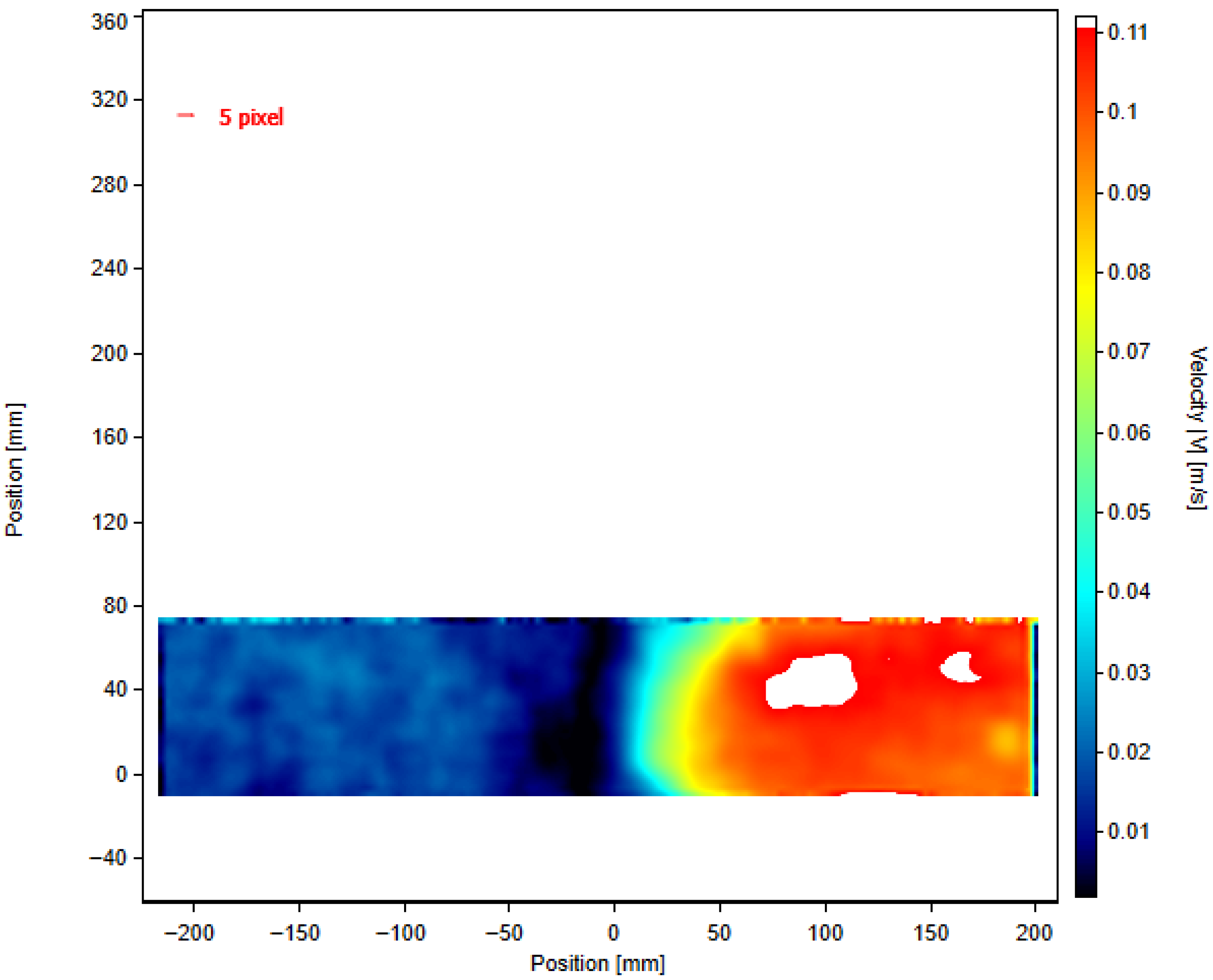
Flow characterisation was performed using planar Particle Image Velocimetry (PIV), providing both the mean velocity field and the standard deviation of the streamwise velocity component. The mean velocity map (Figure 4) clearly shows the influence of the plate on the incoming turbulent flow. Upstream of the plate, the average flow speed is approximately . In the vicinity of the plate, the flow is significantly decelerated, with local minima reaching about , indicating the relevant reduction in velocity due to the presence of the plate. Downstream, the velocity slightly recovers due to the small clearance left between the plate and the water tunnel walls to prevent flow blockage.

Figure 4.
Contour map of the mean velocity field . The blurry region represents the portion of the domain above the water free surface, which is excluded from the PIV measurement area.
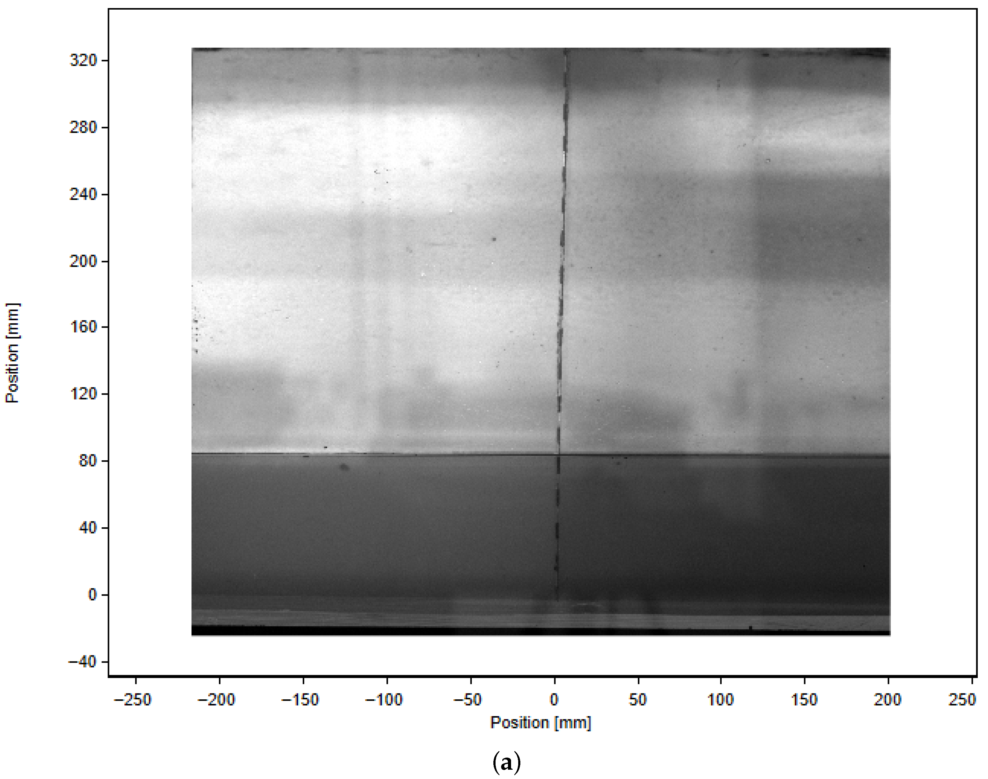
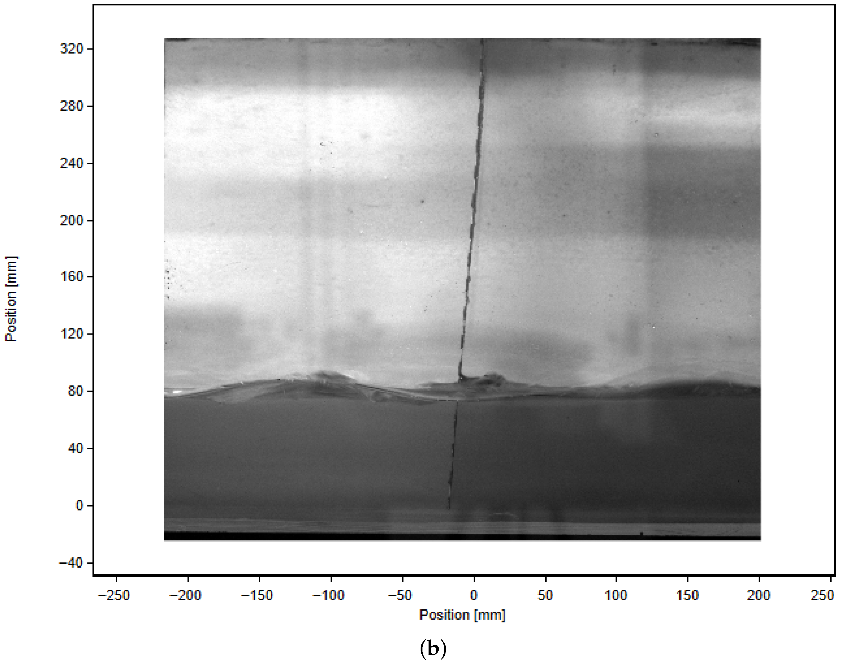
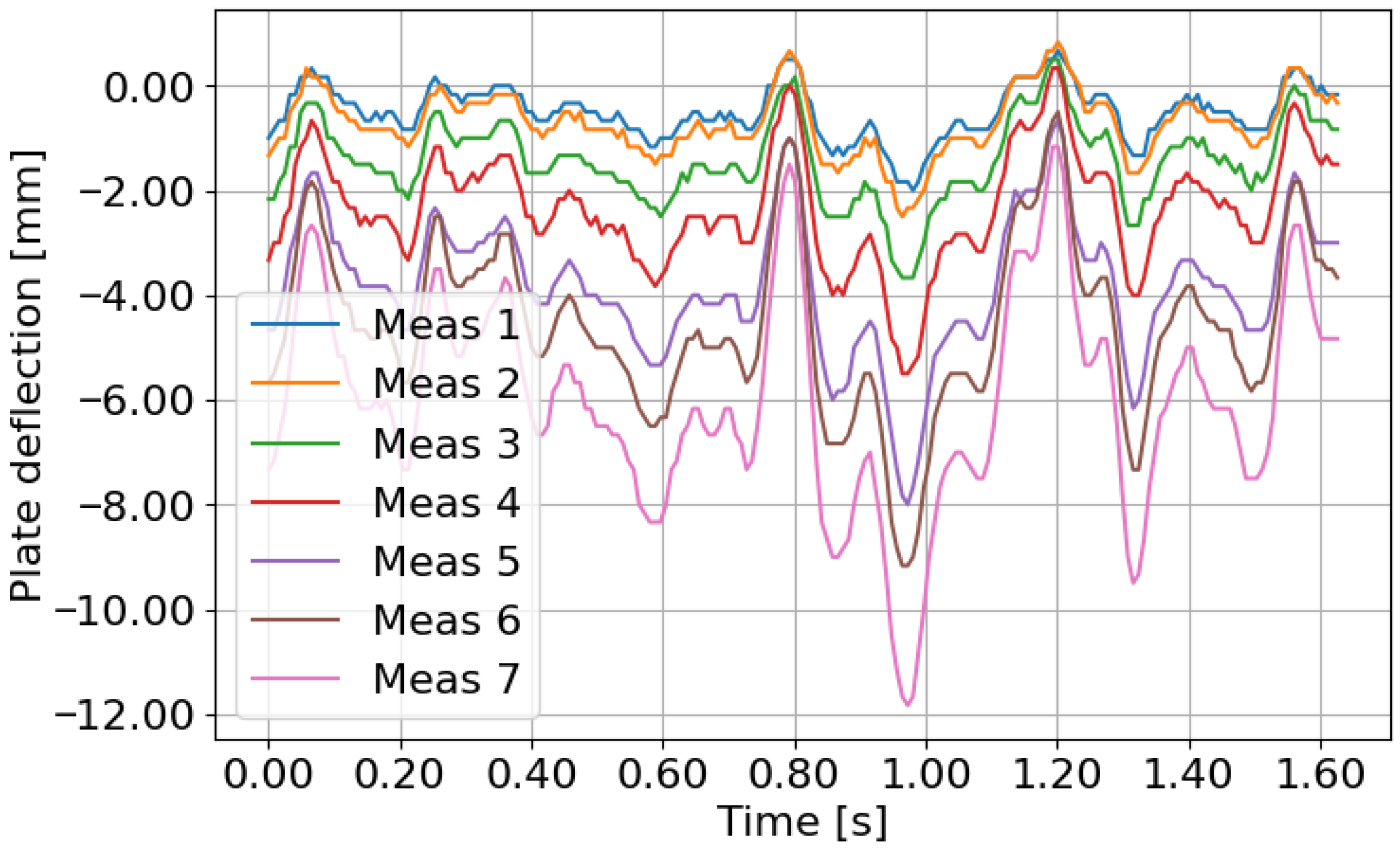
In parallel with the flow field analysis, the displacements of the aluminium plate were evaluated according (see Figure 5) to the methodology described in Section 3. The analysis focused exclusively on the x-displacement component, corresponding to the mid-plane deflection of the plate. Measurements were taken at the seven markers used as inputs for the reconstruction algorithm and at the three verification markers employed for accuracy assessment. Figure 6 shows the time history of the deflections recorded at the seven measurement points. These data provide a direct link between the flow-induced loading patterns observed in the PIV measurements and the structural response captured through the deflection time series.
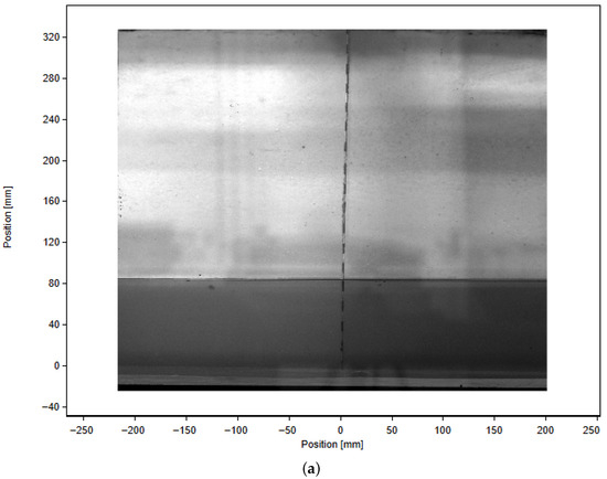
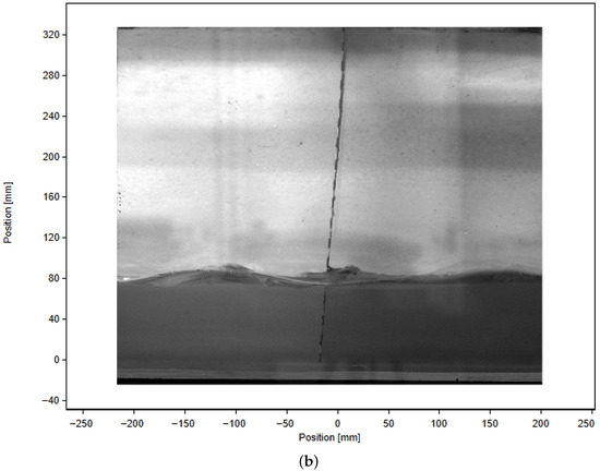
Figure 5.
Plate visualisation for displacement measurements: (a) Undeformed shape. (b) Deformed shape.
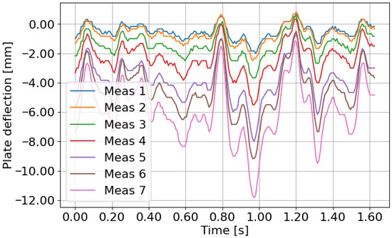
Figure 6.
Measured x-displacements (mid-plane deflections) at the seven input markers used in the modal reconstruction algorithm.
4.2. Modal Reconstruction
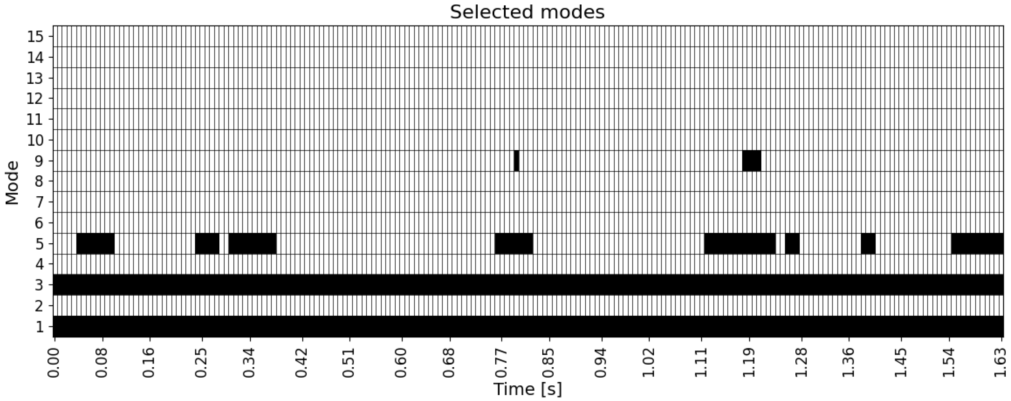
The proposed SHM framework is designed to reconstruct the full-field deformation of the plate from sparse measurements while simultaneously validating the structural state by monitoring locations not directly involved in the reconstruction process. Figure 7 depicts the modes retained at each timestep considered, obtained by feeding the signals from the seven measurement sensors into the random forest ML classifier. Notably, the highest retained mode corresponds to the ninth. To further assess the framework’s performance, three validation markers, located near the water’s free surface, were excluded from the reconstruction input set and used exclusively for independent verification.
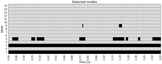
Figure 7.
Retained modes for each timestep obtained by the random forest ML classifier.
For each validation marker, two complementary indicators are considered:
- 1
- The time history of the reconstructed deflection compared with the corresponding experimental measurements using image-based tracking;
- 2
- The instantaneous difference, in millimetres, between reconstructed and measured deflections, representing the monitoring residual.
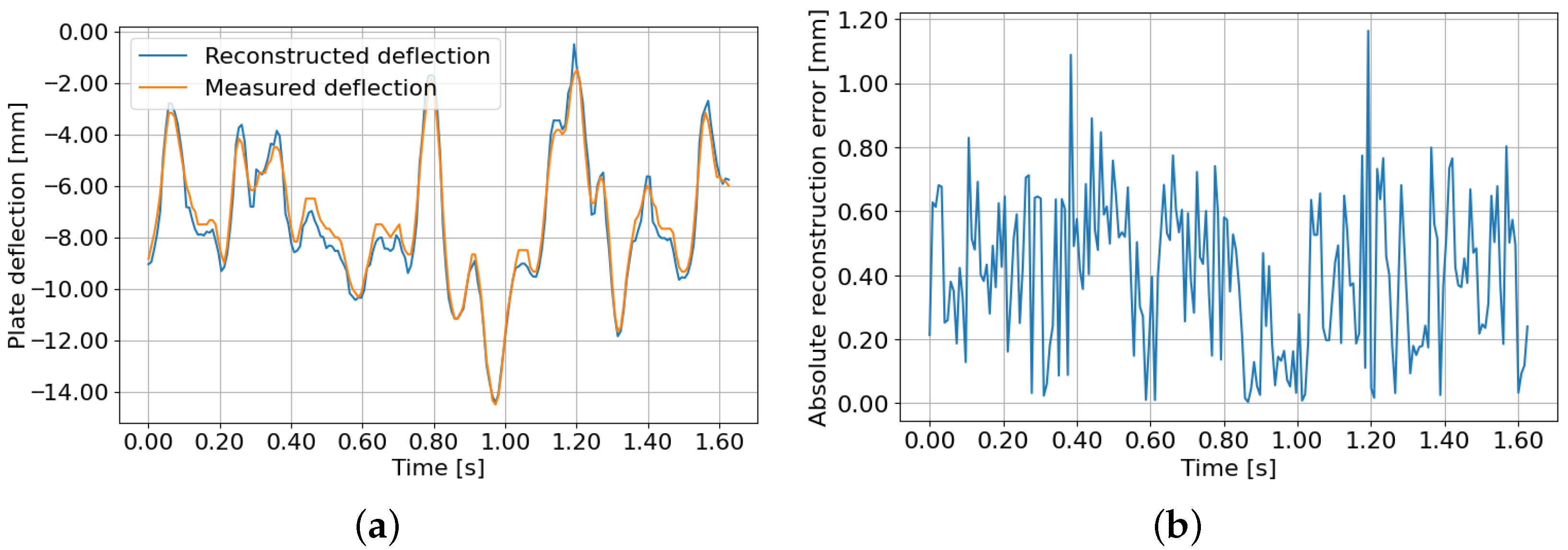
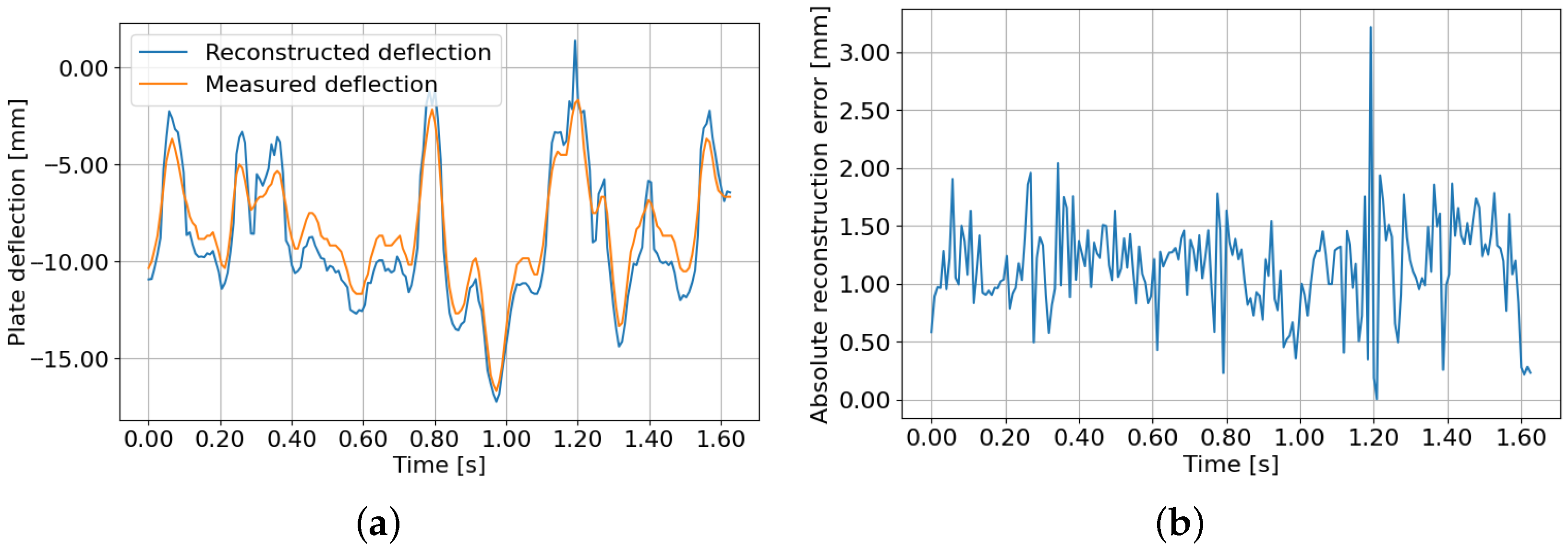
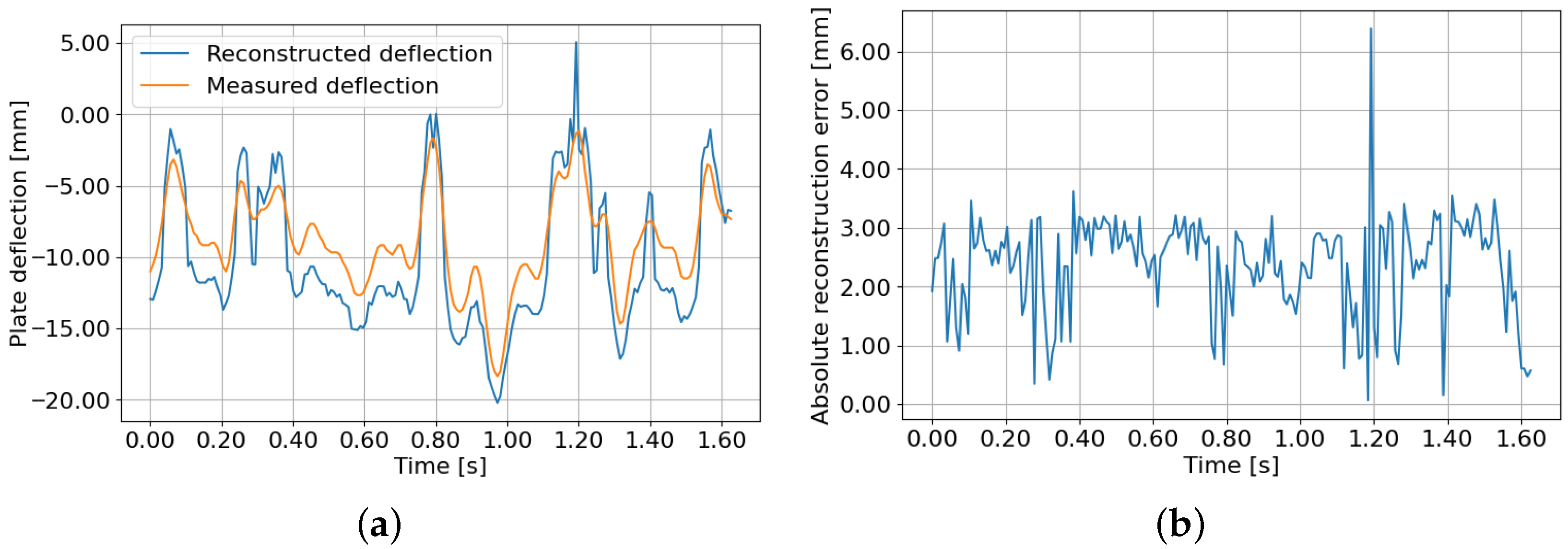
Figure 8, Figure 9 and Figure 10 present the results for the three validation markers. In each figure, subfigure (a) shows the direct comparison between the reconstructed and measured deflection histories, while subfigure (b) depicts the temporal evolution of the monitoring residual.
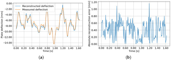
Figure 8.
Validation results for Marker 1: (a) Experimental vs. reconstructed deflection over time. (b) Monitoring residual in millimetres.
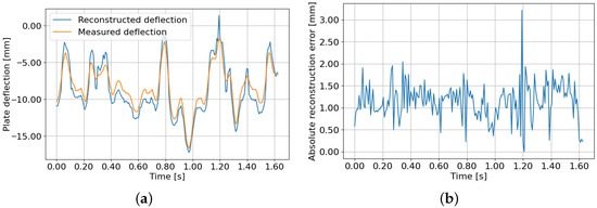
Figure 9.
Validation results for Marker 2: (a) Experimental vs. reconstructed deflection over time. (b) Monitoring residual in millimetres.
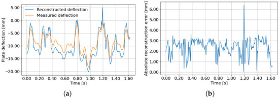
Figure 10.
Validation results for Marker 3: (a) Experimental vs. reconstructed deflection over time. (b) Monitoring residual in millimetres.
Finally, Table 1 reports, for each verification marker, the RMSE and NRMSE calculated over the entire time interval, comparing the measured and reconstructed deflections. As expected, the further a marker is located from the measurement points, the higher the RMSE and NRMSE values, reaching 2.51 mm and 14.64%, respectively, for the last marker. This behaviour can be mitigated by increasing the number of measurement points, which introduces more linearly independent equations for the modal decomposition, allowing more modes to be retained and improving reconstruction accuracy. Alternatively, reconstruction can be enhanced by improving the performance of the pseudoinverse used in computing modal coordinates.

Table 1.
RMSE and NRMSE for each verification marker over the entire time interval.
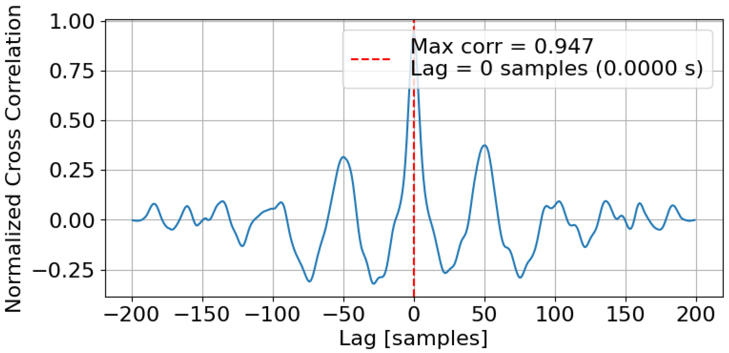
To strengthen the validation, we have included the results of the normalised cross-correlation for each verification marker. The maximum values are 0.990, 0.972, and 0.947 for Markers 1, 2, and 3, respectively. These high values indicate strong agreement in the temporal evolution and overall shape of the reconstructed signals compared with the experimental measurements, confirming the reliability of the reconstruction even for markers located farther from the measurement points. The slight decrease in cross-correlation for the third marker is consistent with the higher NRMSE, reflecting the increased difficulty of accurately reconstructing regions more distant from the sensors.
Figure 11, Figure 12 and Figure 13 present the normalised cross-correlation plots for the three validation markers, illustrating both the peak correlation and the relative temporal alignment between measured and reconstructed signals.
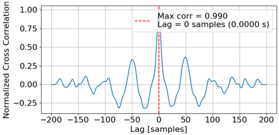
Figure 11.
Normalised cross-correlation between measured and reconstructed deflections for Marker 1.

Figure 12.
Normalised cross-correlation between measured and reconstructed deflections for Marker 2.

Figure 13.
Normalised cross-correlation between measured and reconstructed deflections for Marker 3.
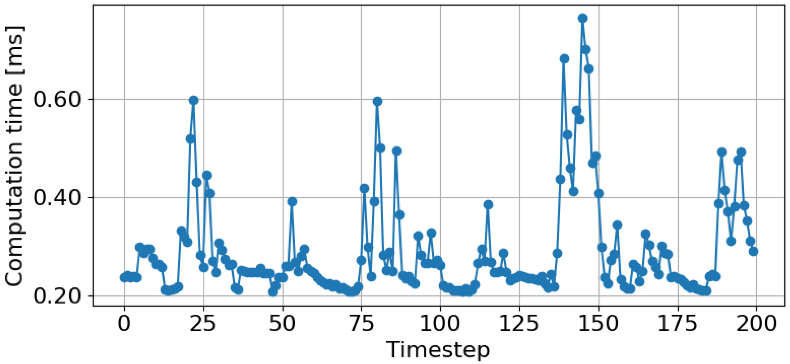
The computational performance of the full-field reconstruction algorithm over the entire mesh is illustrated in Figure 14. Peaks in computation time correspond to timesteps where the largest number of modes is retained. The average computation time is 0.239 ms, while the maximum observed is 0.642 ms. These results demonstrate that the proposed approach is computationally efficient and suitable for real-time or near-real-time SHM applications.
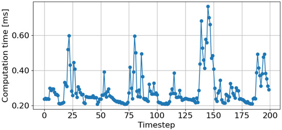
Figure 14.
Computation time per timestep for the full-field reconstruction of the plate, highlighting peaks when more modes are retained.
5. Conclusions
This study presented an experimental and numerical framework for reconstructing the full-field deformation of a flexible aluminium plate operating under unsteady fluid loading in a water tunnel. The proposed methodology integrates sparse displacement measurements, acquired via a digital CMOS camera, with a modal reconstruction approach informed by mode selection based on strain energy contribution. A random forest classifier, trained on a synthetic database generated from a high-fidelity digital twin, was employed to map sparse sensor data to modal coordinates, enabling accurate SHM from limited measurements.
The experimental setup allowed for the tracking of seven measurement markers for reconstruction and three independent verification markers for accuracy assessment. The reconstructed deflections showed good agreement with the camera-measured signals at the verification markers, with reconstruction errors remaining within a few tenths of a millimetre, demonstrating the robustness of the approach under realistic fluid–structure interaction conditions.
Flow visualisation using planar PIV provided a complementary global estimate of the flow loading on the plate, clearly highlighting the local flow deceleration in its vicinity.
Overall, the integrated methodology, combining visualisation, modal reconstruction, and machine learning, proved effective for real-time deformation monitoring of partially submerged flexible structures. This approach offers a strong foundation for developing SHM systems in marine and hydraulic engineering, particularly where direct full-field measurements are impractical. Future work will focus on extending the method to multi-directional displacement components, implementing adaptive mode selection strategies, and performing in situ validation under operational conditions.
Author Contributions
Conceptualisation, G.L., S.M. and P.F.; methodology, G.L.; software, G.L. and S.M.; validation, G.L., S.M. and P.F.; formal analysis, G.L., S.M. and P.F.; investigation, G.L., S.M. and P.F.; resources, G.L., S.M. and P.F.; data curation, G.L., S.M. and P.F.; writing—original draft preparation, G.L. and S.M.; writing—review and editing, G.L.; visualisation, S.M. and P.F.; supervision, P.F.; project administration, P.F.; funding acquisition, P.F. All authors have read and agreed to the published version of the manuscript.
Funding
This research received no external funding.
Institutional Review Board Statement
Not applicable.
Informed Consent Statement
Not applicable.
Data Availability Statement
The raw data supporting the conclusions of this article will be made available by the authors on request.
Conflicts of Interest
The authors declare no conflicts of interest.
References
- Strzalka, C.; Marinkovic, D.; Zehn, M.W. Stress mode superposition for a priori detection of highly stressed areas: Mode normalisation and loading influence. J. Appl. Comput. Mech. 2021, 7, 1698–1709. [Google Scholar] [CrossRef]
- Wang, M.; Sheng, X. Combining empirical wavelet transform and transfer matrix or modal superposition to reconstruct responses of structures subject to typical excitations. Mech. Syst. Signal Process. 2022, 163, 108162. [Google Scholar] [CrossRef]
- Semblat, J.F.; Duval, A.M.; Dangla, P. Modal superposition method for the analysis of seismic-wave amplification. Bull. Seismol. Soc. Am. 2003, 93, 1144–1153. [Google Scholar] [CrossRef]
- Gao, Z.; Zhao, M.; Du, X.; Wang, J. Effective-mode superposition response spectrum method for three dimensional seismic response analysis of underground structures. Soil Dyn. Earthq. Eng. 2023, 174, 108161. [Google Scholar] [CrossRef]
- Fulici, M.; Belardi, V.; Dalla Palma, M.; Liuzzo, G.; Paoletti, D.; Vivio, F.; Fanelli, P. Effects of seismic isolation on the dynamic behaviour of the DTT torus complex during earthquake events. Fusion Eng. Des. 2024, 203, 114476. [Google Scholar] [CrossRef]
- Yeager, M.; Todd, M.; Gregory, W.; Key, C. Assessment of embedded fiber Bragg gratings for structural health monitoring of composites. Struct. Health Monit. 2017, 16, 262–275. [Google Scholar] [CrossRef]
- Esposito, M.; Gherlone, M. Composite wing box deformed-shape reconstruction based on measured strains: Optimization and comparison of existing approaches. Aerosp. Sci. Technol. 2020, 99, 105758. [Google Scholar] [CrossRef]
- Choi, S.M.; Kim, M.H. Shape reconstruction from partially missing data in modal space. Comput. Graph. 2002, 26, 701–708. [Google Scholar] [CrossRef]
- Yang, J.; Fu, Z.; Zou, Y.; He, X.; Wei, X.; Wang, T. A response reconstruction method based on empirical mode decomposition and modal synthesis method. Mech. Syst. Signal Process. 2023, 184, 109716. [Google Scholar] [CrossRef]
- Horas, C.S.; De Jesus, A.M.; Ribeiro, D.; Calçada, R. Efficient multiscale methodology for local stress analysis of metallic railway bridges based on modal superposition principles. Eng. Fail. Anal. 2022, 138, 106391. [Google Scholar] [CrossRef]
- Cui, J.; Zeng, J.; Shao, F.; Wang, S.; Liu, S.; Huang, Y.; Tang, S. Reconstruction of composite panel deformation based on modal superposition and calibration method by fiber optic sensors. In Proceedings of the First Conference on Distributed Optical Fiber Sensing Technology and Applications (DOFS 2024); SPIE: Bellingham, DC, USA, 2025; Volume 13654, pp. 327–339. [Google Scholar] [CrossRef]
- Fanelli, P.; Biscarini, C.; Jannelli, E.; Ubertini, F.; Ubertini, S. Structural health monitoring of cylindrical bodies under impulsive hydrodynamic loading by distributed FBG strain measurements. Meas. Sci. Technol. 2017, 28, 024006. [Google Scholar] [CrossRef]
- Bogert, P.; Haugse, E.; Gehrki, R. Structural shape identification from experimental strains using a modal transformation technique. In Proceedings of the 44th AIAA/ASME/ASCE/AHS/ASC Structures, Structural Dynamics, and Materials Conference, Norfolk, VA, USA, 7–10 April 2003; p. 1626. [Google Scholar]
- A new modal superposition method for nonlinear vibration analysis of structures using hybrid mode shapes. Mech. Syst. Signal Process. 2018, 107, 317–342. [CrossRef]
- Ferhatoglu, E.; Cigeroglu, E.; Özgüven, H.N. A novel modal superposition method with response dependent nonlinear modes for periodic vibration analysis of large MDOF nonlinear systems. Mech. Syst. Signal Process. 2020, 135, 106388. [Google Scholar] [CrossRef]
- Schwarz, B.J.; Richardson, M.H. Linear superposition and modal participation. In Proceedings of the Topics in Modal Analysis I, Volume 7: Proceedings of the 32nd IMAC, A Conference and Exposition on Structural Dynamics, 2014; Springer: Berlin/Heidelberg, Germany, 2014; pp. 161–172. [Google Scholar] [CrossRef]
- Liuzzo, G.; Parisi, M.; Fanelli, P. Modal Shapes Selection Criterion for Modal Reconstruction Aimed at Structural Health Monitoring. Eng. Proc. 2025, 85, 39. [Google Scholar] [CrossRef]
- APDL, A.M. Elements Reference ANSYS, Release 2020 R2; Ansys Inc.: Southpointe, PA, USA, 2020. [Google Scholar]
- Cheng, Y.; Li, Z.; Wang, G.; Peng, C.; Zhang, L.; Yang, W.; Jiang, M.; Sui, Q. Strain field reconstruction of crossbeam structure based on load–strain linear superposition method. Smart Mater. Struct. 2021, 30, 075020. [Google Scholar] [CrossRef]
- Cheng, Y.; Zhang, L.; Jiang, M.; Sui, Q. Strain/displacement field reconstruction and load identification of high-speed train load-bearing structure based on linear superposition method. IEEE Trans. Instrum. Meas. 2022, 71, 7003408. [Google Scholar] [CrossRef]
- Li, Z.; Cheng, Y.; Zhang, L.; Wang, G.; Ju, Z.; Geng, X.; Jiang, M. Strain field reconstruction of high-speed train crossbeam based on FBG sensing network and load-strain linear superposition algorithm. IEEE Sensors J. 2021, 22, 3228–3235. [Google Scholar] [CrossRef]
- Li, J.; Li, S.; Cheng, Y.; Wang, Y.; Zhang, L.; Zhang, F.; Jiang, M. Deformation and load detection of wing structure based on load-strain linear superposition. IEEE Trans. Instrum. Meas. 2025, 74, 7005611. [Google Scholar] [CrossRef]
- Li, L.; Zhong, B.S.; Geng, Z.Y.; Sun, W. Structural Shape Reconstruction of FBG Flexible Plate Using Modal Superposition Method. In Proceedings of the International Design Engineering Technical Conferences and Computers and Information in Engineering Conference, Cleveland, OH, USA, 6–9 August 2017; American Society of Mechanical Engineers: New York, NY, USA, 2017; 58226, p. V008T12A038. [Google Scholar] [CrossRef]
- Liuzzo, G.; Parisi, M.; Fanelli, P. Analytical Formulation of New Mode Selection Criteria in the Reconstruction of Static Deformation of Structures Through Modal Superposition. Appl. Mech. 2025, 6, 67. [Google Scholar] [CrossRef]
- Casini, P.; Vasta, M. Scienza Delle Costruzioni, 4th ed.; CittàStudi: Milan, Italy, 2019. [Google Scholar]
- Timoshenko, S.; Goodier, J. Theory of Elasticity, 2nd ed.; McGraw-Hill Book Company: New York, NY, USA, 1951. [Google Scholar]
- Hodson, T.O. Root mean square error (RMSE) or mean absolute error (MAE): When to use them or not. Geosci. Model Dev. Discuss. 2022, 2022, 1–10. [Google Scholar] [CrossRef]
Disclaimer/Publisher’s Note: The statements, opinions and data contained in all publications are solely those of the individual author(s) and contributor(s) and not of MDPI and/or the editor(s). MDPI and/or the editor(s) disclaim responsibility for any injury to people or property resulting from any ideas, methods, instructions or products referred to in the content. |
© 2025 by the authors. Licensee MDPI, Basel, Switzerland. This article is an open access article distributed under the terms and conditions of the Creative Commons Attribution (CC BY) license (https://creativecommons.org/licenses/by/4.0/).


