Abstract
The stability of time-dependent compressible linear flows, which are characterized by periodic variations in either their shape or their shear, is investigated. Two novel parametric instabilities are found: an instability that occurs for periodically wobbling elliptic vortices at a number of discrete oscillation frequencies that are proportional to the Mach number and an instability that occurs for all linear flows at various frequencies of the shear oscillation that depend on the Mach number. In addition, the physical mechanism underlying the instabilities is explained in terms of the linear interaction of three waves with time-varying wavevectors that describe the evolution of perturbations: a vorticity wave representing the evolution of incompressible perturbations and two counter-propagating acoustic waves. Elliptical instability occurs because the scale of the acoustic waves decreases exponentially and their wave action is conserved, leading to an exponential increase in the acoustic waves’ energies. The instability in shear-varying flows is driven by the interaction between vorticity and the acoustic waves, which couple through the shear and for specific frequencies resonate parametrically, leading to exponential or linear growth.
1. Introduction
Since the seminal works of Kraichnan [1] and Lighthill [2], it has been established that acoustic waves and turbulent flows interact in complex ways. This interaction is bidirectional: Sound propagation is influenced by turbulence and vortical flows [3,4], while acoustic waves can trigger instabilities in mixing layers or jets [5,6]. Therefore, the investigation of incipient instabilities in compressible flows and of their underlying physical mechanisms is an active field of research [7,8,9,10] with many engineering applications [11,12].
A class of idealized flows that have been studied extensively because they can serve as a local approximation for the features of both incompressible and compressible turbulence is that of linear flows [13]. This class includes those with elliptical streamlines, representing strained vortices [14], the extensively studied Couette flow [15], and extensional flows that are crucial in many physical processes [16,17,18]. The advantage of these flows is that their stability properties and dynamics can be easily addressed, shedding light into important physical mechanisms. In this context, analytic solutions for the evolution of small amplitude perturbations in incompressible steady flows were obtained, and the physical mechanisms underlying elliptic [19,20,21] and hyperbolic instabilities [22], as well as the transient growth in the case of plain Couette flows [23,24], were identified.
Some of these results were extended to compressible steady flows. In the case of Couette flow, it was shown that at low Mach numbers the perturbations manifest as a superposition of propagating acoustic waves, which grow linearly with time, and aperiodic vorticity waves [25]. An interaction between vorticity and acoustic waves was also identified: Vorticity perturbations were found to extract energy from the shear and then transfer it to the acoustic waves, exciting them at a certain amplitude [26]. Analytic estimates for the amplitude of the excited acoustic waves via vortical perturbations showed that the excitation is exponentially weak for low Mach numbers, but it is of order one for moderate Mach numbers [27]. The analysis regarding the transient growth of perturbations for the Couette flow was extended to moderate [28] and large Mach numbers [29], as well as to a perfect gas model [30]. It was also extended to the cases of elliptical and extensional flows, where it was found that the intuitive decomposition of the perturbations into acoustic and vorticity waves holds in the low Mach number limit with similar interactions occurring [31].
The stability properties of linear time-dependent flows have received much less attention despite the fact that, in most applications, the flows are time-varying. By considering the evolution of incompressible perturbations in the low Mach number limit, Mansour and Lundgren [32] and Leblanc and Le Penven [33] found parametric instabilities in unbounded circular or elliptical vortices that were periodically compressed on their plane. In addition, it has been shown that the core of a vortex can be destabilized via the periodic compression of acoustic waves [34,35]. Similar instabilities were also found for a gas in a rotating cylinder undergoing axial periodic compressions [36]. However, a thorough investigation into the evolution of compressible perturbations across the entire class of linear flows that are time-dependent is still lacking. This work aims to fill that gap.
In particular, we investigate the stability of circular, elliptic, Couette, and hyperbolic flows, for which their shapes or shears vary periodically in time. This includes wobbling elliptic or hyperbolic flows, pulsating Couette flows, and circular and elliptic flows with a time-dependent orientation. The analysis is performed by expressing the imposed perturbations as spatial Fourier waves with time-dependent wavenumbers and amplitudes, known as Kelvin modes or shear waves [37]. This method was first applied over a century ago in viscous shear flows [37,38] and has since been widely utilized for both laboratory [39,40] and geophysical flows [41,42,43]. It was also generalized to arbitrary flows in the works of Eckhoff [44] and Lifschitz and Hameiri [45], who developed the geometrical optic stability method. We discover two novel parametric instabilities: one occurring in periodically wobbling elliptic vortices and another one occurring in all linear flows when their shear varies periodically. In addition, we investigate the physical mechanisms underlying the instabilities in terms of the interaction between the vortical flow and acoustic waves. It is shown that elliptical instability arises from the parametric growth of acoustic waves’ wavenumbers combined with the conservation of their wave action, while the instabilities in shear-varying flows are due to parametric resonance between the vortical flow and the waves as they are coupled by the shear.
This paper is organized as follows: In Section 2, we derive the equations governing the evolution of small-amplitude perturbations and the resulting ODEs for the evolution of the amplitudes and wavevectors of the Kelvin modes. In Section 3 and Section 4, we investigate the stability of flows with periodically varying types and shears, respectively. We finally end with our conclusions in Section 5.
2. Perturbation Evolution for a Wide Class of Time-Varying Linear Flows
We consider the following class of planar, time-dependent flows:
These vary linearly in space , where the star denotes dimensional variables, the dagger denotes the matrix transpose, and is the following shear matrix:
The velocity field with components describes a wide class of linear, two-dimensional flows that occur for different values of parameters and , and they are illustrated in Figure 1. The parameter is a function of the ratio of the strain over the vorticity of the flow [] and describes the type of the flow: For , the flow is circular (Figure 1a); for , the flow is elliptic with eccentricity (Figure 1b), and the value corresponds to a plane Couette flow (Figure 1c); for , the flow is hyperbolic (Figure 1d,e). The parameter is the shear rate , and its norm describes the magnitude of the shear (for example, in Couette or hyperbolic flows), while its sign describes the orientation of the flow (for example, clockwise or counter-clockwise in elliptic flows). This class of flows includes wobbling elliptic or hyperbolic flows when varies with time, pulsating Couette flows when varies with time, and circular and elliptic flows with a time-dependent orientation when changes its sign as well. The goal of this work is to address the stability of these time-varying flows when compressibility is taken into account.
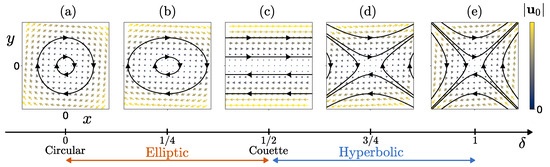
Figure 1.
The class of linear flows described by Equation (1). The curves show the streamlines of the flow and vectors in the velocity field. (a) (circular flow), (b) (elliptic flow), (c) (Couette flow), (d) (hyperbolic flow), and (e) (hyperbolic flow). In all panels, .
Assuming that we concentrate within the limit of vanishing viscocity, the mean flow satisfies the Euler equations:
where and are the constant background density and pressure fields of the homentropic flow, and is an external forcing term that models all relevant mechanisms generating the time-dependent flow in a simplistic manner. For instance, in the case of a plane Couette flow, it models the time-dependent variation in the boundaries producing the flow in the presence of viscocity. We consider small-amplitude, planar-compressible perturbations of density and velocity around the mean flow, which are assumed to be isentropic. The evolution of the perturbations is governed by the linear equations
The equations are non-dimensionalized, using a length scale to be determined for the position vector, the adiabatic speed of sound as a velocity scale, as the time scale, and and as the density and pressure scales, respectively. The non-dimensional perturbations denoted without the star evolve according to
where the non-dimensional density perturbations are equal to the pressure perturbations. The Mach number is based on the maximum value of the time-dependent shear. Therefore the non-dimensional shear is bounded by one ().
To solve for the perturbation’s evolution, we employ the Kelvin non-modal method [28,31,37], which transforms Equations (6) and (7) into a system of ODEs. The steps for this transformation are as follows. First, we define a new system of coordinates that follow Lagrangian trajectories, which are given as the solution to the following equation:
Defining , the convected coordinates are given in terms of the original coordinates through the linear transformation:
Differentiating and using (8), we find that is given by the solution to the equation
with being the identity matrix. In these coordinates, the material derivative is simply the time derivative
As a result Equations (6) and (7) become spatially homogeneous, and we can seek solutions in the form of plane waves
where is the wave vector. Since there is no intrinsic spatial scale for the unbounded, linear flows considered, we choose the length scale to be , where is the dimensional wave vector. In this case, the wave vector is of unit norm and can be written in terms of the angle that the phase lines form with the normal direction:
By substituting the plane-wave solutions (12) into Equations (6) and (7) and using the transformation given in (9), we find that and satisfy the following system of ODEs:
where
The inner product is preserved due to Equations (9), and (16) and is therefore the time-dependent wavenumber in the initial coordinate with component and an initial value .
The system of Equations (14)–(16) yields the time-evolution of the perturbations. The energy density of the perturbations that is given by
evolves according to the non-dimensional strain and the Reynolds stress:
where denotes the Hermitian transpose.
The stability of the flow is addressed by rewriting the system of ODEs in the compact form
where is the state vector and
and then, by numerically calculating the propagator that furnishes the solution:
As the energy density of the perturbations is proportional to the Euclidean norm for the flow-state vector
the stability of the flow for both short and long time scales can be investigated by performing a singular value decomposition of the propagator [46]:
The non-modal, transient growth of perturbations at short or finite time scales can be addressed by calculating the square of the first singular value at a target finite time (), which is the largest energy growth attained over this interval [23,47]. The optimal perturbation achieving this growth is the corresponding first column of , while the evolved perturbation at the target time is the first column of . Optimal transient growth can also be equivalently assessed via the finite time Lyapunov exponent:
In the small time asymptotic limit addressing the instantaneous explosive growth of perturbations, the largest singular value is the largest real eigenvalue of approximating the propagator, while the optimal perturbation and the corresponding instantaneous Lyapunov vector coincide. For the linear flows considered in this work, the propagator is independent of the wavevector in the small time limit. The growth then depends only on the flow parameters and is proportional to the non-dimensional strain S:
while the corresponding instantaneous Lyapunov vector is . The asymptotic stability of the flow can be addressed by calculating the first singular value in the limit of large times, which corresponds to the first Lyapunov exponent:
The corresponding Lyapunov vector is the first column of , while the first column of is the initial perturbation exciting the Lyapunov vector with the largest amplitude [46].
WKB Solution in the Limit of Small Mach Number and the WKB Base
For the case of steady Couette flow [27], as well as for the more general class of linear flows considered here [31], much of the dynamics were exemplified by an asymptotic WKB solution in the limit of a small Mach number. Such a solution is possible in the case of Equations (14) and (15) as well, as the adiabatic dynamics found by Favraud and Pagneux [31] for slowly varying flows hold even when varies with time.
The WKB solution is based on the fact that the flow evolves for small Mach numbers () on a slow time scale . Introducing the slow time scale in Equation (19) yields the following:
where
is the zeroth order dynamical operator and
contains the dynamics at next order. We can therefore write solution in the form of an asymptotic series expansion:
Plugging the expansion into (27) yields, for the leading order, an eigenvalue problem. The solutions to this problem are the following order-0 WKB modes:
with . The mode is divergence-free and corresponds to the solution in the incompressible limit that is typically referred to as a vorticity mode or a vorticity wave [27]. The mode is irrotational. In the limit of no flow (), they represent two counter-propagating acoustic waves with wavenumber and unit phase speeds. In the low-Mach-number limit, their wavenumber evolves slowly over time while their phase evolves over the fast time scale .
An additional advantage of the WKB solution, is that these three modes form a basis on which the exact solution can be written for any Mach number. That is,
where is the time-dependent amplitude of the vortical and acoustic parts of the perturbation. By substituting (32) into (27) and after performing some manipulations, Favraud and Pagneux [31] found that the time evolution of the amplitudes is governed by
where
while the perturbation energy density (17) is written in terms of the three modes as
The matrix describes the interaction of the three modes that can influence each other in two ways. They can change the phase of the other waves, speeding them up or slowing them down, or they can change their amplitude (enhancing or hindering the other waves).
The analysis of the perturbation evolution in the order-0 WKB basis allows us to identify the two pathways by which perturbations grow. The first is through the dynamics of the vorticity and acoustic waves exemplified by the case of waves with constant or almost constant amplitude. In this case, it is evident from Equation (35) that the energy of the modes can grow either transiently or asymptotically when the wavenumber grows/decays. As will be shown in Section 3, this mechanism underlies the parametric instability in type-varying flows ( and constant ). The second pathway is through the interaction between the vorticity and acoustic waves, which is described by Equation (33) and can modify the amplitudes of the waves even if the wavenumber is constant or bounded. As will be shown in Section 4, the parametric instabilities arising in shear-varying flows ( and constant ) occur due to this mechanism.
3. Stability Analysis of Type-Varying Flows
In this section, we study the stability of flows with time-varying types, i.e., , and constant shear . We consider periodic variations of the form
around a mean value with frequency and strength . As was noted before, the stability of a type-varying flow is reflected in the evolution of the perturbation wave vector. Using Equations (10) and (16), we find that the components of satisfy
Rescaling time and introducing the parameters and reduces (38) to the usual form of the Mathieu equation [48]:
It is well known that the Mathieu equation has both stable and unstable solutions depending on its parameters values [49] and describes many stabilization and destabilization phenomena like the Kapitza pendulum [50]. Similarly for the time-dependent flows investigated here, such parametric growth of the wavevector can stabilize or destabilize the flows as the elliptic flow is stable when is constant while the hyperbolic flow is unstable [31].
3.1. Destabilization of Elliptic Flows
When the modulation frequency is close to a resonant frequency with , the solutions of the Mathieu Equation (38) grow exponentially due to parametric instability [48,49]. As an illustration, we present in Figure 2a the norm that is calculated via the numerical integration of (10) for a wobbling elliptic flow with periodically varying eccentricity () when . The observed growth of the norm is also accompanied by an exponential growth of the energy of the perturbations, as shown in Figure 2b. In order to investigate this growth, we analyze the solution in terms of the WKB-base, which is in terms of the dynamics of the vorticity and acoustic waves.
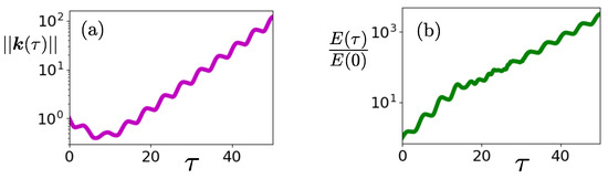
Figure 2.
Evolution of (a) the wavevector norm and (b) the energy growth of the perturbations for an elliptic flow with periodically varying eccentricities. Eccentricity is modulated around with strength and frequency , where and . In both panels, the angle is , and the initial conditions are .
The amplitudes of the acoustic waves shown in Figure 3a initially oscillate and asymptotically approach a constant value. The reason is that the terms in Equation (34) involving the interaction of the acoustic waves with the vorticity wave are monotonically decreasing functions of the norm of the wavevector, and the interactions cease when the norm starts to become large. In addition, the terms involving the interaction of the two acoustic waves are proportional to , and for the extremely rapidly varying phase of the waves, this term yields zero tendencies on average. On the other hand, the wave action of the perturbations
shown in Figure 3b converges asymptotically to a constant value, suggesting that the energy of the perturbations increases exponentially at the same rate as the norm of the wavevector.
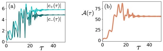
Figure 3.
(a) The amplitude of the two acoustic waves and (b) the wave action for an elliptic flow with periodically varying eccentricities. The flow parameters are as in Figure 2.
This result is verified by the stability analysis of the propagator. The finite-time Lyapunov exponent calculated through a singular value decomposition of the propagator (cf. Equation (24) ) is shown in Figure 4a. For short times, we observe large transient growth comparable to the average value of instantaneous growth, which is for the parameters chosen (cf. Equation (25) ), and then, it decreases rapidly while oscillating with frequency . For large times, we observe that it behaves as an asymptote relative to half the finite-time Lyapunov exponent of the norm of the wavevector that is also shown.
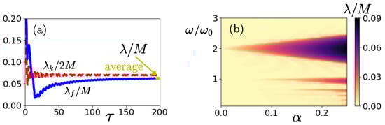
Figure 4.
(a) Evolution of the finite-time Lyapunov exponent of (14)–(16) (solid line) and half of the finite-time Lyapunov exponent of the norm of the wavevector (dashed line). (b) First Lyapunov exponent as a function of frequency and strength of the modulation. It is also noted that the Lyapunov exponent is an even function of . In both panels, the mean flow-type parameter is , and .
The first Lyapunov exponent of the parametric instability is calculated by averaging over a period of the oscillation relative to large times () (yellow line in Figure 4a). We find that it does not depend on the initial angle of the phase lines ( the same does not hold for the optimal perturbations exciting the Lyapunov vector with the maximum amplitude that depends strongly on ) but depends on the modulation frequency and strength. This is illustrated in Figure 4b where the first Lyapunov exponent is shown as a function of frequencies and with the range of values for the modulation strength () being such that the flow remains elliptical (). The detected regions of exponential instability match with the Arnold tongues of the Mathieu equation. To investigate the possibility of large transient growth or unbounded algebraic growth in the asymptotically stable regions between the Arnold tongues, we calculated the finite time Lyapunov exponent at moderate () to large () times for the range of stable frequencies. Low values of growth were found for all values of and within the asymptotically stable region.
3.2. Stabilization of Hyperbolic Flows
Motivated by the fact that shape-varying elliptic flows are destabilized by the parametric growth of the wavenumber satisfying the Mathieu equation, we explore the possible stabilization of hyperbolic flows via the time modulation of their shape, as exemplified by a time-varying strain. The reason for this is that hyperbolic flows are unstable for steady flows due to the same mechanism (the exponential growth of acoustic waves associated with the corresponding growth of their wavenumber) [31] and the Mathieu equation that governs the evolution of the component of the wavenumber allows for stable solutions in a certain parameter range.
Indeed, it is known [51] that when , i.e., , stable solutions of the Mathieu equation exist if , i.e., . Namely, stable solutions can exist if there is a time period when (see Equation (36)), suggesting that hyperbolic flow can be stabilized by periodic variations in its shape only if it becomes elliptic at certain time intervals. To verify this, we plot in Figure 5a the maximum Lyapunov exponent as a function of modulation frequency and strength for a value of , satisfying the inequality above within the range of modulation strength considered. We observe that is positive when as the inequality above is not satisfied, i.e., . For satisfying the stability inequality, there is a narrow tongue with (light areas), with this area becoming wider as the strength is increased. As in the case of elliptic instability, we calculated the finite time Lyapunov exponent for large times in order to investigate the possibility of large transient growth or unbounded algebraic growth in the asymptotically stable region. An example of the energy evolution is shown in Figure 5b, where we observe that the perturbation energy undergoes periodic intervals of moderate transient amplification but remains bounded.
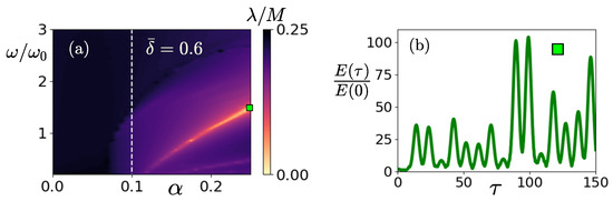
Figure 5.
Stabilization of hyperbolic flows by periodic modulation of their shape. (a) The maximum Lyapunov exponent as a function of the normalized frequency and the strength of the modulation for , , and . (b) Energy growth of a perturbation for and , for which [this is shown by the square in panel (a)]. The initial conditions are as shown in Figure 2.
4. Stability Analysis of Shear-Varying Flows
In this section, we investigate the stability of flows with time-varying shear and constant flow-type . The temporal modulations in the shear are assumed to be periodic:
where is the frequency of the modulation. For the elliptic and hyperbolic flows, this means that their rotation changes periodically with time, without a change in their eccentricity or strain, respectively, while for Couette flows, this means a periodically changing shear.
Exponential instability is found for all Mach numbers and in contrast to the parametric instability for type-varying flows; in this case, there is a strong dependence of the growth rate on the initial angle , where the phase lines form with respect to the normal direction. For low Mach numbers, the dependence of the first Lyapunov exponent on the frequency of the modulation and the angle is shown in Figure 6. For elliptic flow, we observe one narrow tongue of instability around the frequency and the same holds for the case of Couette flow. The hyperbolic flow exhibits two instability tongues centered around and . For both types of flows, the growth rate for is maximized for angles and , while the corresponding instability for occurs for a band of angles close to .
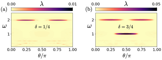
Figure 6.
(a,b) The first Lyapunov exponent in the cases of (a) an elliptic flow () and (b) a hyperbolic flow () with a periodically modulated shear as a function of the frequency of the modulation and the angle of the initial wavevector. In both panels, .
In order to examine whether the instability is associated with the growth of the wavevector as with type-varying flows, we calculate the wavevector that is given by the following expression:
The norm of the wavevector shown in Figure 7a for the cases of elliptic, Couette, and hyperbolic flows is almost constant at an initial value of one, with small-amplitude (order M) oscillations having modulation frequency in all three cases. However, the norm of the amplitude of the downstream propagating acoustic wave plotted in Figure 7b diverges exponentially, as well as the amplitude of the other acoustic waves and the vorticity wave. We therefore conclude that it is the interaction between the acoustic and vorticity waves that drives the parametric instability in this case.
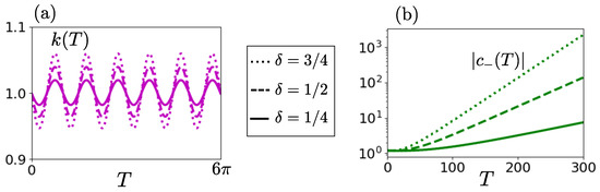
Figure 7.
Evolution of (a) the norm of the wave vector of the perturbations and (b) the norm of the amplitude of the acoustic wave for an elliptic flow with (solid lines), for a Couette flow (dashed lines), and for a hyperbolic flow with (dotted lines). In both panels, and , and the frequency is . In (b), the initial conditions are .
A better understanding of the instability can be achieved by noting that while the shear flow oscillates on the fast time scale, the wavenumber evolves on the time scale that is slow for low Mach numbers. Therefore, the WKB modes can be approximated to the first order, evolving in the absence of a mean flow with constant wavenumber :
That is, the vorticity wave is approximately constant while the acoustic waves have unit frequencies. We can thus look for solutions to Equation (19), comprising at leading order of the WKB modes with a slowly varying amplitude and higher-order corrections:
Substituting in (19), we obtain, for the leading order in M, vorticity and acoustic waves with constant amplitudes. The growth of these waves is obtained by calculating the Reynolds stress (giving the energy tendency) from the leading order solution, furnishing some algebra:
Secular terms arise for two resonant frequencies. The first is , for which we have resonance between the varying shear and the interaction of the vorticity with the acoustic waves (last term in (45) ). The second is , for which we have resonance between the varying shear and the acoustic waves [second term in (45)]. This is subharmonic since the frequency of the acoustic waves is equal to one. It is shown in Appendix A, where a two-time scale solution is formally obtained, and the growth rate for the resonant frequency is
while the growth rate for is given by the following:
The comparison between the Lyapunov exponent calculated from the numerical integration of Equations (14)–(16) and the asymptotic expressions given in Equations (46) and (47) illustrated in Figure 8 shows excellent agreement. Note that for , instability is indeed observed only for hyperbolic flows and for a band of angles close to as the condition
should be satisfied for positive growth rates. For , instability is observed for all three classes of flow, with the growth rate being the maximum for phase lines forming an angle with respect to the streamwise direction. Note also that for both frequencies, the growth rate is proportional to the Mach number and is an increasing function of .
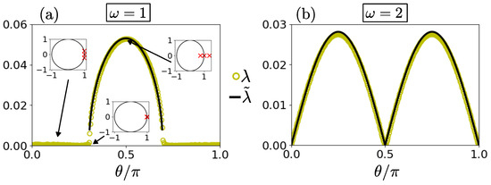
Figure 8.
Comparison of the Lyapunov exponent (circles) for (a) and (b) with the estimate (solid lines) given by Equations (46) and (47), respectively. In the inset panels, the crosses denote the eigenvalues of the monodromy matrix of Equation (23) in the complex plane, computed for the angle shown by the arrows. In both panels, and .
Finally, there are two special cases of linear growth of perturbations for . The first case occurs for the angle satisfying equality (48). In Appendix A, it is shown that for these angles, the amplitude of the vorticity wave grows linearly, while the amplitudes of the acoustic waves are constant. This means that in the limiting case of Couette flow, even though there is no exponential growth, the flow is asymptotically unstable with the linear growth of streamwise-independent () perturbations. The special case of linear growth can also be verified by calculating the propagator matrix given in (23) that was found to be periodic with period . The eigenvalues of the monodromy matrix, i.e., the propagator calculated over one period, are shown in the complex plane in the insets of Figure 8a for three angles. When the flow is stable, the eigenvalues lie in the unit circle in the complex plane (solid line), while when the flow is unstable, one eigenvalue lies outside of this disk. At the point where the transition from stability to instability occurs, the eigenvalues coalesce, forming an exceptional point of order 2 and leading to linear growth. Such a behavior is typical in non-Hermitian systems and is known to occur in many physical systems [52,53]. The second case occurs for the limiting hyperbolic flow with , where we show in Appendix A that, for any initial angle , we obtain linear growth for the amplitudes of the acoustic waves, while the amplitude of the vorticity wave is constant.
In order to see how these resonances are achieved, we look at the interaction of the three modes given by the elements of . The influence of each wave on the others depends on its phase difference or with respect to the other waves, which is almost linearly varying with time in the limit of low Mach numbers. Therefore, if the shear is constant, each wave has a zero net effect on the other waves’ amplitudes. This occurs, for example, in the case of the shape-varying flows examined in Section 4, where the rapidly varying phase leads to constant amplitudes. But in this case, this effect is negated when the shear oscillates at resonant frequencies, facilitating a non-zero interaction between the waves, which can mutually grow on a slow time-scale.
Some of the results found above for weakly compressible flows hold in the case of larger Mach numbers as well. This is shown in Figure 9a, illustrating the first Lyapunov exponent as a function of the Mach number and the frequency of the oscillation in the case of Couette flows. We observe that the subharmonic resonance initially widens with increasing Mach numbers, and for , there is an additional resonance at frequency . For , the two bands around and form a single broad band of instability while smaller band resonances at even lower frequencies appear. In Figure 9b, which illustrates the dependence of the growth rate on the angle for , it is shown that both the subharmonic resonance and the resonance at are optimal for angle , while the lower frequency resonances occur for various values of the angle.
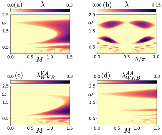
Figure 9.
Couette flow (). (a) The first Lyapunov exponent as a function of frequency and Mach number M. (b) The first Lyapunov exponent as a function of frequency and angle . The Mach number is . (c,d) The first Lyapunov exponent computed by the reduced dynamics (49) and (50), respectively. In panels (a,c,d), angle .
To investigate additional resonances, we utilize the solution in terms of the WKB base. As the resonances for low Mach numbers are due to different wave interactions, we consider two reduced dynamics of Equation (33). The first is to consider the reduced matrix
in which we ignore the interaction of the two acoustic waves. The second is to consider the reduced matrix
in which the interaction of only the two acoustic waves is taken into account. Figure 9c,d show the first Lyapunov exponent obtained from the two reduced dynamics (49) and (50), and , respectively. The comparison of these growth rates to the growth rate in Figure 9a shows that the instabilities at low frequencies are due to the interaction of vorticity with the acoustic waves in the presence of shear, while the subharmonic resonance arises due to the interaction of the two acoustic waves even for moderate Mach numbers.
Similar results are found for elliptic flows, as illustrated in Figure 10, where it is shown that the additional band that appears around occurs in this case as well (Figure 10a), with the growth rate being the maximum for (Figure 10b). The bands around the subharmonic resonance and the lower frequency band merge and disappear when . However, the resonances appearing at lower frequencies () that are similar to those observed in the Couette flow persist for larger Mach numbers. Additionally, Figure 10c,d, which show the Lyapunov exponents and as functions of and M, suggest that the interaction of the two acoustic waves generates the subharmonic resonances again, while the inclusion of the vorticity wave in the dynamics gives rise to the remaining resonances at lower frequencies.
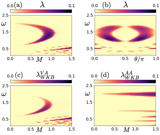
Figure 10.
(a–d): Same as in Figure 9 for an elliptic flow with .
The dependence of the parametric instability on the Mach number for hyperbolic flows is shown in Figure 11. The subharmonic resonance with the growth rate maximized for and the harmonic resonance with the growth rate maximized for persist for moderate Mach numbers, with similar characteristics and the same mechanisms driving the instability. The only differences compared to lower Mach numbers are a broadening of the resonant bands and a slight shift towards larger frequencies. Finally, the additional low-frequency resonances occurring for several values of the angle that were found for the other two classes of linear flows are observed in this case as well.
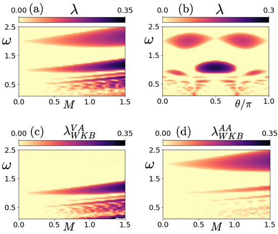
Figure 11.
(a–d): Same as in Figure 9 for a hyperbolic flow with .
5. Conclusions
In this work, the linear stability of a broad class of time-varying linear flows was investigated with respect to planar compressible perturbations. The class of flows considered includes circular, elliptic, Couette, and hyperbolic flows, and they were assumed to either vary periodically in shape (for example, elliptic flows with periodically varying eccentricity or hyperbolic flows with periodically varying strain) or to have a periodically varying shear (for example, elliptic flows with periodically varying orientations or pulsating Couette flows).
The stability of the flow was addressed via a singular value decomposition of the propagator for the temporal evolution of the amplitude of plane waves with time-dependent wavenumbers (Kelvin modes). Two novel parametric instabilities were found. The first is elliptic instability with respect to planar acoustic waves for vortices that wobble periodically at resonant frequencies proportional to the Mach number with the corresponding growth rates also being proportional to the Mach number. The second occurs for all linear flows in the case of periodically varying shear. For low Mach numbers, two resonances, a harmonic and a subharmonic one, were identified. The subharmonic resonance manifests for all classes of linear flows, while the harmonic resonance manifests as exponential instability for hyperbolic flows and as linear instability for Couette flows. The growth rate of the perturbations in the cases of both harmonic and sub-harmonic resonances is proportional to the Mach number and has a strong dependence on the angle that the phase lines of the perturbations form with the normal direction. In the case of harmonic resonance, the growth rate is maximized for streamwise-independent perturbations, and we thus expect the emergence of streaks in the flow. In the case of subharmonic resonance we expect the emergence of perturbations oriented at an angle with respect to the normal direction. For larger Mach numbers, a second almost harmonic resonance appears for Couette and elliptic flows. The band of resonant frequencies widens around the two main resonances for all linear flows and for moderate Mach numbers, and a single resonant region of frequencies is formed, while other resonances for smaller frequencies appear as well.
The physical mechanisms underlying the two parametric instabilities were revealed by writing the perturbations as a superposition of three waves: a vorticity wave that corresponds to the solution in the incompressible limit and two acoustic waves with a time-dependent phase. It was shown that the perturbations can grow due to two pathways. The first is through changes in their wavenumber, leading to energy growth for the waves even when their amplitude is constant. The second is through the interactions of the three waves that can change their phase speeds and their amplitudes.
Parametric elliptic instability was found to be driven by the first pathway: the scale of the waves decreases exponentially due to the parametric growth of particle trajectories caused by the periodically wobbling vortex. As the wave action of the acoustic modes is conserved, this leads to exponential growth. For the case of periodically varying shear, instability occurs due to the second pathway: Vorticity and acoustic waves are coupled by time-dependent shear, with the influence of each wave on the others depending on its phase difference with the other waves. For a constant shear, the amplitude tendency varys sinusoidally at the rate of the time-dependent phase speed of the acoustic waves, leading to a zero net effect on the other waves’ amplitudes. However, when the shear oscillates at resonant frequencies, it negates this effect and facilitates a non-zero interaction between the waves, which can mutually grow. The subharmonic resonance was found to be due to the interaction of acoustic waves, while harmonic resonance and the resonances at lower frequencies occur as the vortical part of the flow generates acoustic waves that do not passively propagate, as in Lighthill-like radiation, but they feed back to the vortical part of the flow to produce instability. A stability analysis with respect to three-dimensional perturbations in order to investigate how the mechanisms involving acoustic waves and their dynamics compare to other resonances for elliptic and hyperbolic flows will be pursued in future works.
Author Contributions
Conceptualization, I.K. and N.A.B.; methodology, N.A.B.; software, I.K.; validation, N.A.B.; formal analysis, I.K. and N.A.B.; investigation, I.K. and N.A.B.; writing—original draft preparation, I.K. and N.A.B.; writing—review and editing, N.A.B.; visualization, I.K.; supervision, N.A.B. All authors have read and agreed to the published version of the manuscript.
Funding
I.K. received financial support from the Institut d’Acoustique—Graduate School of Le Mans for conducting this work.
Institutional Review Board Statement
Not applicable.
Informed Consent Statement
Not applicable.
Data Availability Statement
The original contributions presented in the study are included in the article, further inquiries can be directed to the corresponding author.
Acknowledgments
The authors would like to thank Vincent Pagneux for fruitful discussions. I.K. acknowledges hospitality at the University of Ioannina during the period when this work was conducted.
Conflicts of Interest
The authors declare no conflicts of interest.
Abbreviations
The following abbreviations are used in this manuscript:
| ODEs | Ordinary differential equations. |
Appendix A. Analytical Estimate of the Growth Rate for Low Mach Numbers in the Case of Periodically Varying Shear
In this Appendix, we derive analytical estimates for the growth of perturbations in the case of periodically varying shear when the Mach number is small (). The key assumption is that the shear oscillates at the finite frequency while the wavevector that is given by Equation (42) is a slowly varying function of time for low Mach numbers and can be approximated by its initial value . As a result, the phase can be approximated as
while the leading order in the interaction coefficients in (34) is
After the approximation and restoration of the fast time scale , Equation (33), governing the interaction of the three waves, becomes the following:
It is obvious that there are two time scales: the short time scale T for acoustic waves and the shear and long time-scale for the tendency of the amplitude. We therefore use a two-time scale approximation for the solution:
with the time derivative being . Carrying out substitutions in Equation (A5) and equating the orders in M yield, at , leading order terms that are a function of the slow time only, i.e., . At , we obtain the following equation:
where , , and . For and , the secular terms are the slow time derivatives of the amplitudes, and these have to vanish for asymptotic convergence. We thus obtain a constant solution at the leading order in this case, as well as the asymptotic stability of the flow.
For , there are additional secular terms () deriving from the interaction of the vorticity wave with the two acoustic waves. A further simplification can be obtained by noting that if and are real, then for all times and is real for all times. Therefore, we can write, without loss of generality, the system in terms of and only. Assuming the sum of the secular terms to be zero for , we obtain the following equations for the amplitudes of the vorticity and acoustic waves:
For real , the imaginary part of is constant, and we can assume it to be zero without loss of generality. This yields the following second-order equation for :
We thus obtain exponential instability with growth rate when , an inequality that is satisfied only for hyperbolic flow (). There is also the special case of the zero growth rate being satisfied either if () or if (). In the first case, we obtain a constant amplitude for the vorticity wave and linear growth for the acoustic waves.
In the second case, we obtain constant amplitudes for the acoustic waves and linear growth for the vorticity waves:
For , the additional secular terms derive from the interaction of the two acoustic waves. Under the same simplification as above (), the zero sum of the secular terms furnishes the following:
Writing the amplitude in polar form and equating the real and imaginary parts after some algebra, we obtain the following equations for the tendency of the amplitude and the phase:
The first equation has the following solution:
For , that is, for , converges asymptotically to either zero or depending on the initial conditions. For , that is, for , converges to depending again on the initial conditions. Plugging (A16) in (A15) and integrating, we obtain the following:
In the large time’s asymptotic limit, if or if . Therefore, in any case, the growth rate is given by .
References
- Kraichnan, R.H. The scattering of sound in a turbulent medium. J. Acoust. Soc. Am. 1953, 25, 1096–1104. [Google Scholar] [CrossRef]
- Lighthill, M.J. On boundary layers and upstream influence II. Supersonic flows without separation. Proc. R. Soc. A 1953, 217, 478–507. [Google Scholar]
- Landau, L.D.; Lifshitz, E.M. Fluid Mechanics. V.6. Course of Theoretical Physics; Pergamon Press: Oxford, UK, 1987. [Google Scholar]
- Thomas, J. New model for acoustic waves propagating through a vortical flow. J. Fluid Mech. 2017, 823, 658. [Google Scholar] [CrossRef]
- Ho, C.M.; Huerre, P. Perturbed free shear layers. Annu. Rev. Fluid Mech. 1984, 16, 365–424. [Google Scholar] [CrossRef]
- Doshi, P.S.; Ranjan, R.; Gaitonde, D.V. Global and local modal characteristics of supersonic open cavity flows. Phys. Fluids 2022, 34, 034104. [Google Scholar] [CrossRef]
- Chung, T.J.; Sohn, J.L. Interactions of coupled acoustic and vortical instability. AIAA J. 1986, 24, 1582–1596. [Google Scholar] [CrossRef]
- Crawley, M.; Gefen, L.; Kuo, C.W.; Samimy, M.; Camussi, R. Vortex dynamics and sound emission in excited high-speed jets. J. Fluid Mech. 2018, 839, 313–347. [Google Scholar] [CrossRef]
- Islam, M.R.; Shaaban, M.; Mohany, A. Vortex dynamics and acoustic sources in the wake of finned cylinders during resonance excitation. Phys. Fluids 2020, 32, 075117. [Google Scholar] [CrossRef]
- Dai, X. Vortical–acoustic resonance in an acoustic resonator: Strouhal number variation, destabilization and stabilization. J. Fluid Mech. 2021, 919, A19. [Google Scholar] [CrossRef]
- Borée, J.; Miles, C. In-Cylinder Flow. In Encyclopedia of Automotive Engineering; John Wiley & Sons, Ltd.: Chichester, UK, 2014. [Google Scholar]
- Zhao, D.; Li, X. A review of acoustic dampers applied to combustion chambers in aerospace industry. Prog. Aerosp. Sci. 2015, 74, 114–130. [Google Scholar] [CrossRef]
- Cambon, C.; Scott, J.F. Linear and nonlinear models of anisotropic turbulence. Annu. Rev. Fluid Mech. 1999, 31, 1–53. [Google Scholar] [CrossRef]
- Kerswell, R.R. Elliptical instability. Annu. Rev. Fluid Mech. 2002, 34, 83–113. [Google Scholar] [CrossRef]
- Nikolaidis, M.A.; Ioannou, P.J. Synchronization of low Reynolds number plane Couette turbulence. J. Fluid Mech. 2022, 933, A5. [Google Scholar] [CrossRef]
- Stone, H.A.; Leal, L.G. The influence of initial deformation on drop breakup in subcritical time-dependent flows at low Reynolds numbers. J. Fluid Mech. 1989, 206, 223–263. [Google Scholar] [CrossRef]
- Bigio, D.I.; Sangli, A.N. A new measure for drop deformation in extensional flows at low Reynolds number. Phys. Fluids 2024, 36, 023605. [Google Scholar] [CrossRef]
- Ianniruberto, G. Extensional Flows of Solutions of Entangled Polymers Confirm Reduction of Friction Coefficient. Macromolecules 2015, 48, 6306–6312. [Google Scholar] [CrossRef]
- Pierrehumbert, R.T. Universal short-wave instability of two-dimensional eddies in an inviscid fluid. Phys. Rev. Lett. 1986, 57, 2157–2159. [Google Scholar] [CrossRef]
- Bayly, B.J. Three-Dimensional Instability of Elliptical Flow. Phys. Rev. Lett. 1986, 57, 2160–2163. [Google Scholar] [CrossRef]
- Waleffe, F. On the three-dimensional instability of strained vortices. Phys. Fluids A 1990, 2, 76–80. [Google Scholar] [CrossRef]
- Lagnado, R.R.; Phan-Thien, N.; Leal, L.G. The stability of two-dimensional linear flows. Phys. Fluids 1984, 18, 25–59. [Google Scholar] [CrossRef]
- Schmid, P.J.; Henningson, D.S. Stability and Transition in Shear Flows; Springer: New York, NY, USA, 2001. [Google Scholar]
- Theofilis, V. Global Linear Instability. Annu. Rev. Fluid Mech. 2011, 43, 319–352. [Google Scholar] [CrossRef]
- Chagelishvili, G.D.; Rogava, A.D.; Segal, I.N. Hydrodynamic stability of compressible plane Couette flow. Phys. Rev. E 1994, 50, R4283–R4285. [Google Scholar] [CrossRef]
- Chagelishvili, G.D.; Tevzadze, A.G.; Bodo, G.; Moiseev, S.S. Linear mechanism of wave emergence from vortices in smooth shear flows. Phys. Rev. Lett. 1997, 79, 3178–3181. [Google Scholar] [CrossRef]
- Bakas, N.A. Mechanisms underlying transient growth of planar perturbations in unbounded compressible shear flow. J. Fluid Mech. 2009, 639, 479–507. [Google Scholar] [CrossRef]
- Chagelishvili, G.D.; Khujadze, G.R.; Lominadze, J.G.; Rogava, A.D. Acoustic waves in unbounded shear flows. Phys. Fluids 1997, 9, 1955–1962. [Google Scholar] [CrossRef]
- Farrell, B.F.; Ioannou, P.J. Transient and asymptotic growth of two-dimensional perturbations in viscous compressible shear flow. Phys. Fluids 2000, 12, 3021–3028. [Google Scholar] [CrossRef][Green Version]
- Malik, M.; Alam, M.; Dey, J. Nonmodal energy growth and optimal perturbations in compressible plane Couette flow. Phys. Fluids 2006, 18, 034103. [Google Scholar] [CrossRef]
- Favraud, G.; Pagneux, V. Acoustic–vorticity coupling in linearly varying shear flows using the WKB method. Proc. R. Soc. Lond. Ser. A 2013, 469, 20120708. [Google Scholar] [CrossRef]
- Mansour, N.N.; Lundgren, T.S. Three-dimensional instability of rotating flows with oscillating axial strain. Phys. Fluids A 1990, 2, 2089–2091. [Google Scholar] [CrossRef]
- Leblanc, S.; Le Penven, L. Stability of periodically compressed vortices at low Mach number. Phys. Fluids 1999, 11, 955–957. [Google Scholar] [CrossRef]
- Leblanc, S. Destabilization of a vortex by acoustic waves. J. Fluid Mech. 2000, 414, 315–337. [Google Scholar] [CrossRef]
- Leblanc, S. Acoustic excitation of vortex instabilities. Phys. Fluids 2001, 13, 3496–3499. [Google Scholar] [CrossRef]
- Racz, J.P.; Scott, J.F. Parametric instability in a rotating cylinder of gas subject to sinusoidal axial compression. Part 1. Linear theory. J. Fluid Mech. 2008, 595, 265–290. [Google Scholar] [CrossRef]
- Kelvin, L. Stability of fluid motion: Rectilinear motion of viscous fluid between two parallel plates. Philos. Mag. 1887, 24, 188–196. [Google Scholar]
- Orr, W.M. Stability or instability of the steady motions of a perfect fluid. Proc. R. Ir. Acad. 1907, 27, 69–138. [Google Scholar]
- Jiao, Y.; Hwang, Y.; Chernyshenko, S.I. Orr mechanism in transition of parallel shear flow. Phys. Rev. Fluids 2021, 6, 023902. [Google Scholar] [CrossRef]
- Criminale, W.O.; Jackson, T.L.; Joslin, R.D. Theory and Computation in Hydrodynamic Stability; Cambridge University Press: Cambridge, UK, 2018. [Google Scholar]
- Mamatsashvili, G.R.; Avsarkisov, V.S.; Chagelishvili, G.D.; Chanishvili, R.G.; Kalashnik, M.V. Transient Dynamics of Nonsymmetric Perturbations versus Symmetric Instability in Baroclinic Zonal Shear Flows. J. Atmos. Sci. 2010, 67, 2972. [Google Scholar] [CrossRef]
- Onuki, Y.; Joubaud, S.; Dauxois, T. Breaking of Internal Waves Parametrically Excited by Ageostrophic Anticyclonic Instability. J. Phys. Oceanogr. 2023, 53, 1591–1613. [Google Scholar] [CrossRef]
- Salhi, A.; Cambon, C. Magneto-gravity-elliptic instability. J. Fluid Mech. 2023, 963, A9. [Google Scholar] [CrossRef]
- Eckhoff, K.S. On stability for symmetric hyperbolic systems, I. J. Differ. Eq. 1981, 40, 94–115. [Google Scholar] [CrossRef][Green Version]
- Lifschitz, A.; Hameiri, E. Local stability conditions in fluid dynamics. Phys. Fluids A 1991, 3, 2644–2651. [Google Scholar] [CrossRef]
- Farrell, B.F.; Ioannou, P.J. Generalized stability theory. Part II. Nonautonomous operators. J. Atmos. Sci. 1996, 53, 2041–2053. [Google Scholar] [CrossRef]
- Farrell, B.F.; Ioannou, P.J. Generalized stability theory. Part I. Autonomous operators. J. Atmos. Sci. 1996, 53, 2025–2040. [Google Scholar] [CrossRef]
- Nayfeh, A.H. Introduction to Perturbation Techniques; John Wiley & Sons: New York, NY, USA, 2011. [Google Scholar]
- McLachlan, N. Theory and Application of Mathieu Functions; Oxford University Press: London, UK, 1947. [Google Scholar]
- Ruby, L. Applications of the Mathieu equation. Am. J. Phys. 1996, 64, 39–44. [Google Scholar] [CrossRef]
- Brillouin, L. Wave Propagation in Periodic Structures: Electric Filters and Crystal Lattices; Dover Publications: Mineola, NY, USA, 2003. [Google Scholar]
- Heiss, W.D. Exceptional points of non-Hermitian operators. J. Phys. A Math. Gen. 2004, 37, 2455. [Google Scholar] [CrossRef]
- Berry, M.V. Physics of Nonhermitian Degeneracies. Czech. J. Phys. 2004, 54, 1039–1047. [Google Scholar] [CrossRef]


Disclaimer/Publisher’s Note: The statements, opinions and data contained in all publications are solely those of the individual author(s) and contributor(s) and not of MDPI and/or the editor(s). MDPI and/or the editor(s) disclaim responsibility for any injury to people or property resulting from any ideas, methods, instructions or products referred to in the content. |
© 2025 by the authors. Licensee MDPI, Basel, Switzerland. This article is an open access article distributed under the terms and conditions of the Creative Commons Attribution (CC BY) license (https://creativecommons.org/licenses/by/4.0/).