
A Simple Stochastic Parameterization for Reduced Models of Multiscale Dynamics

Abstract
:1. Introduction
2. General Description of the Method
- Order . From the relation in Equation (10a) we determine that , that is, does not depend on y.
- Order . Here we use the relation in Equation (10b) to express in terms of . We denote the flow, generated by Equation (3), by , so that is the solution of Equation (3) forward in time s with the initial condition y, with the obvious identityNow, consider the integralwhere the group property of is used in the second equality. Then, from the first identity in Equation (12), it follows thatand from the second identity in Equation (12) it follows that is in fact an explicit function of , that is, . However, any must obey the transport equationwhere the second identity is due to Equation (11), and which holds for any s including . Combining Equations (13) and (14) at , we obtainFrom the comparison with Equation (10b) it follows that , that is,
- Order . Here observe that does not depend on y, as pointed out above. This means that the average of with respect to the invariant distribution measure of Equation (3) is the identity operation, and the same holds for its τ-derivative. Then, averaging out Equation (10c) with respect to yields,For the first integral above we express the gradient term as a time derivative of the function along the flow (in the same way as above for ):The invariant distribution measure preserves the averages of functions of :This, in turn, results inand, therefore,
Remark: Does not Depend on ε.
3. Practical Implementation of the Reduced Stochastic Model For a General Multiscale Process With Linear Coupling
- First, we are going to presume that the multiscale dynamical system in Equation (27) is not necessarily computable at will for arbitrarily long time intervals. The reason is that if it is possible, then the need for a reduced model becomes somewhat difficult to justify.
- Even if the full multiscale model is not computable at will, we still need some statistical information about it to formulate the reduced model. Here, we presume that some typical state of the slow variables x is available, such that the dynamics evolve in the proximity of . For example, a rough estimate of the mean state of the slow variables of the full multiscale system can be taken as , or a nearby state.
- We presume that the limiting fast dynamics in Equation (28) is computable beyond the mixing time scale, so that time averages of Equation (28) can be computed, at least for a single given value .
The Choice of σ.
4. Computational Study: The Two-Scale Lorenz 96 Model With Linear Coupling
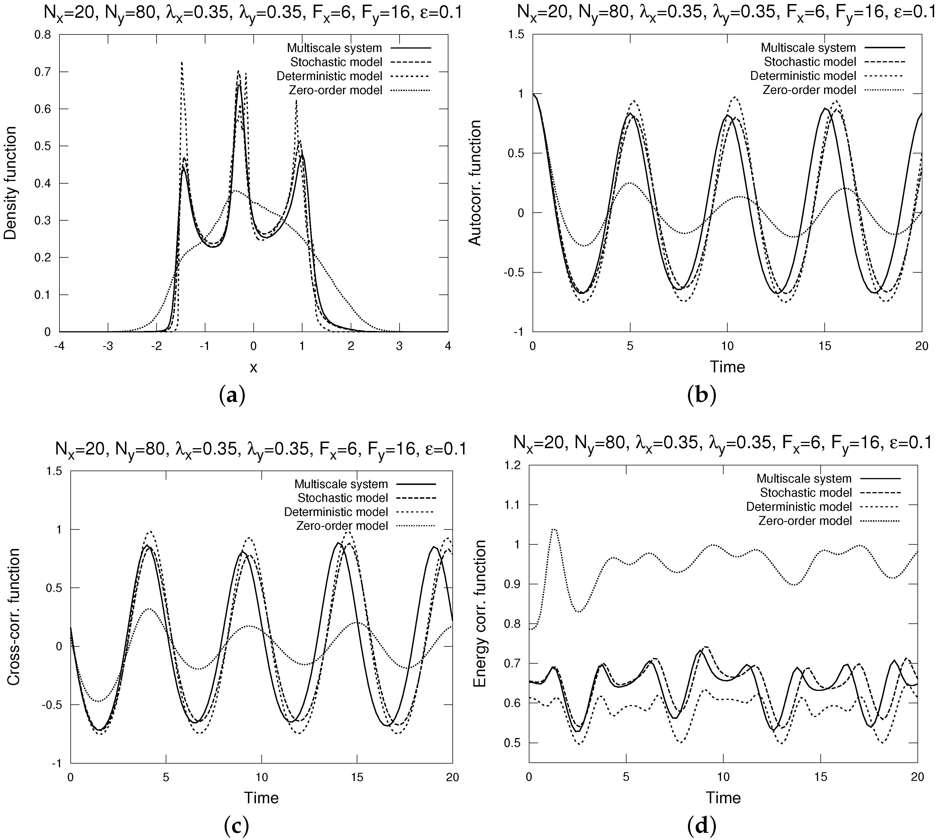
- The complete rescaled Lorenz system from Equations (35a)–(35b);
- The stochastic reduced model from Equation (31);
- The deterministic reduced model obtained from Equation (31) by removing the stochastic forcing (this model was previously developed in [35]);
- The poor man’s version of Equation (31) with no stochastic forcing and the first-order linear deterministic correction term R set to zero (further referred to as the “zero-order” system, same as in [35]). This zero-order system represents the simplest reduced model with constant parameterization of coupling terms.
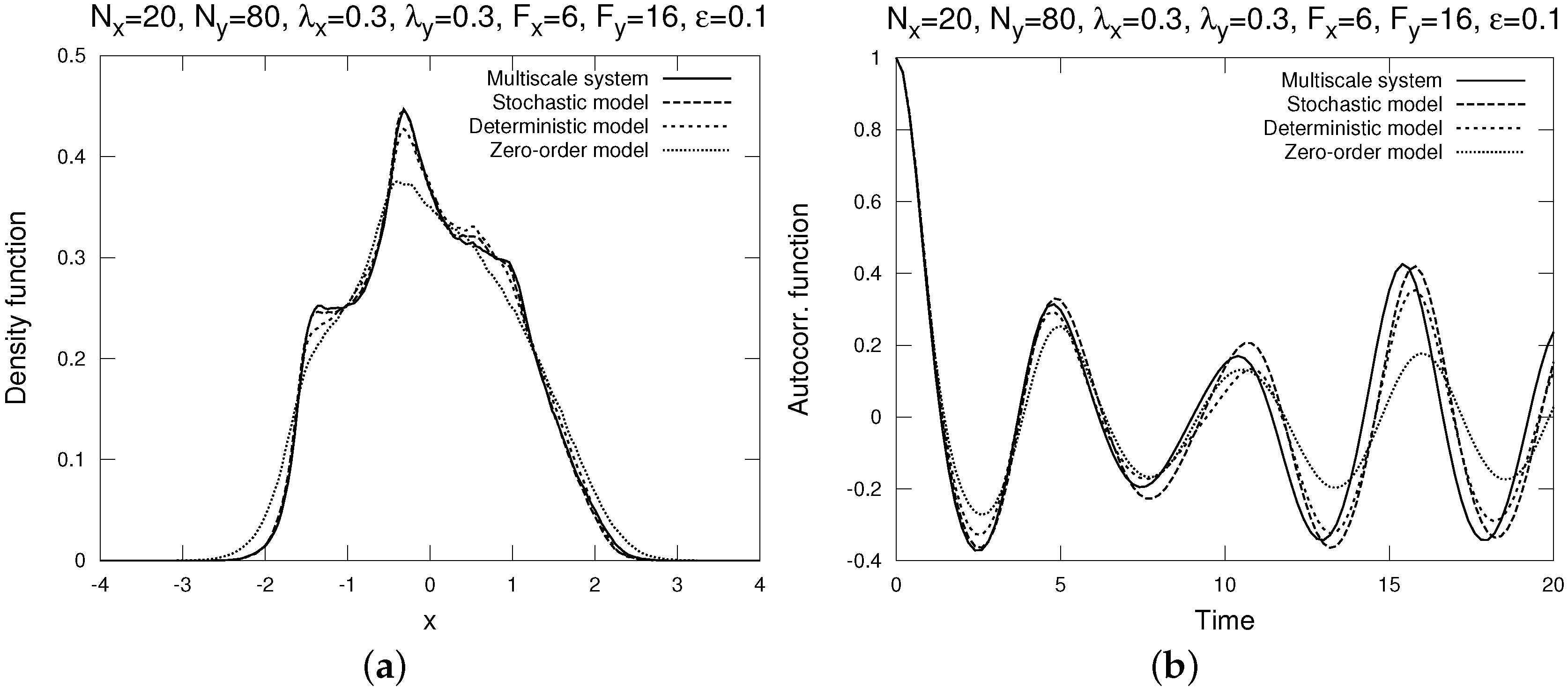
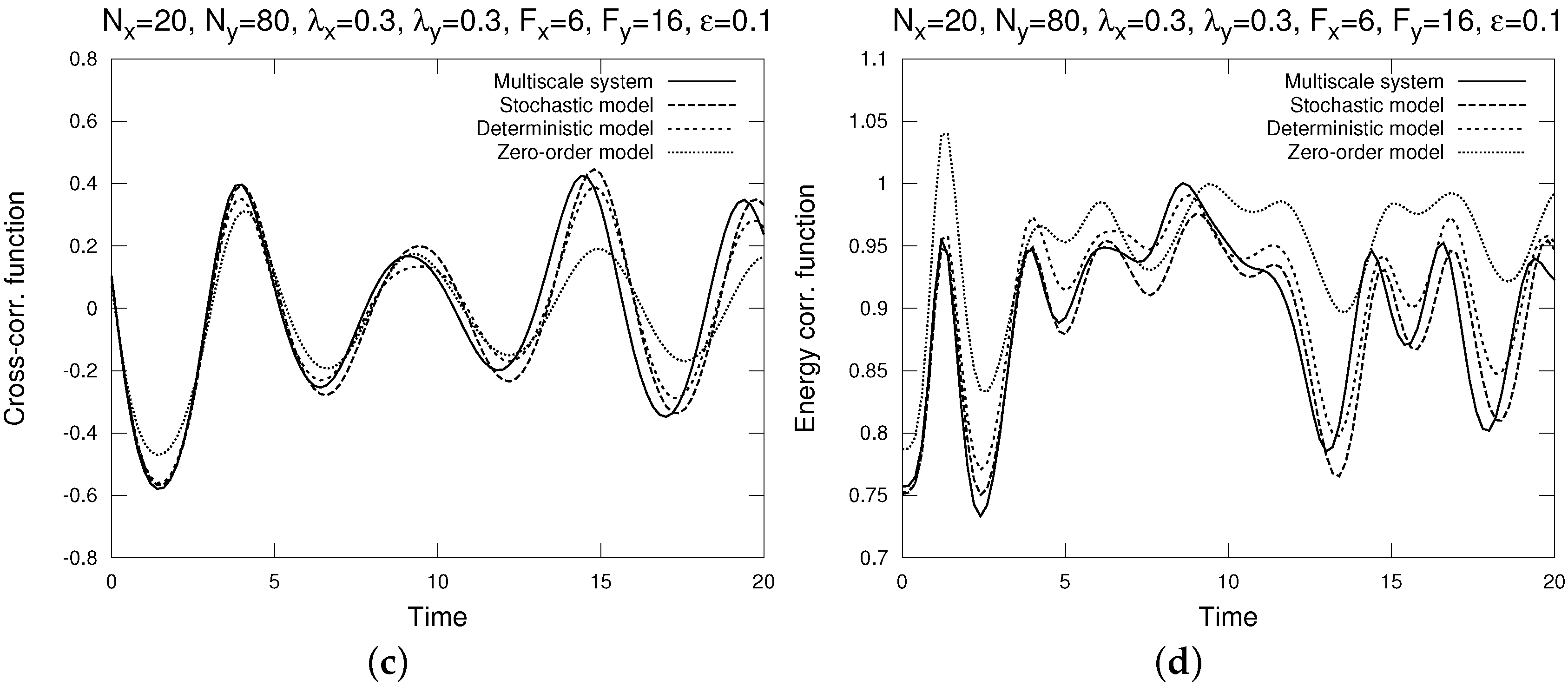
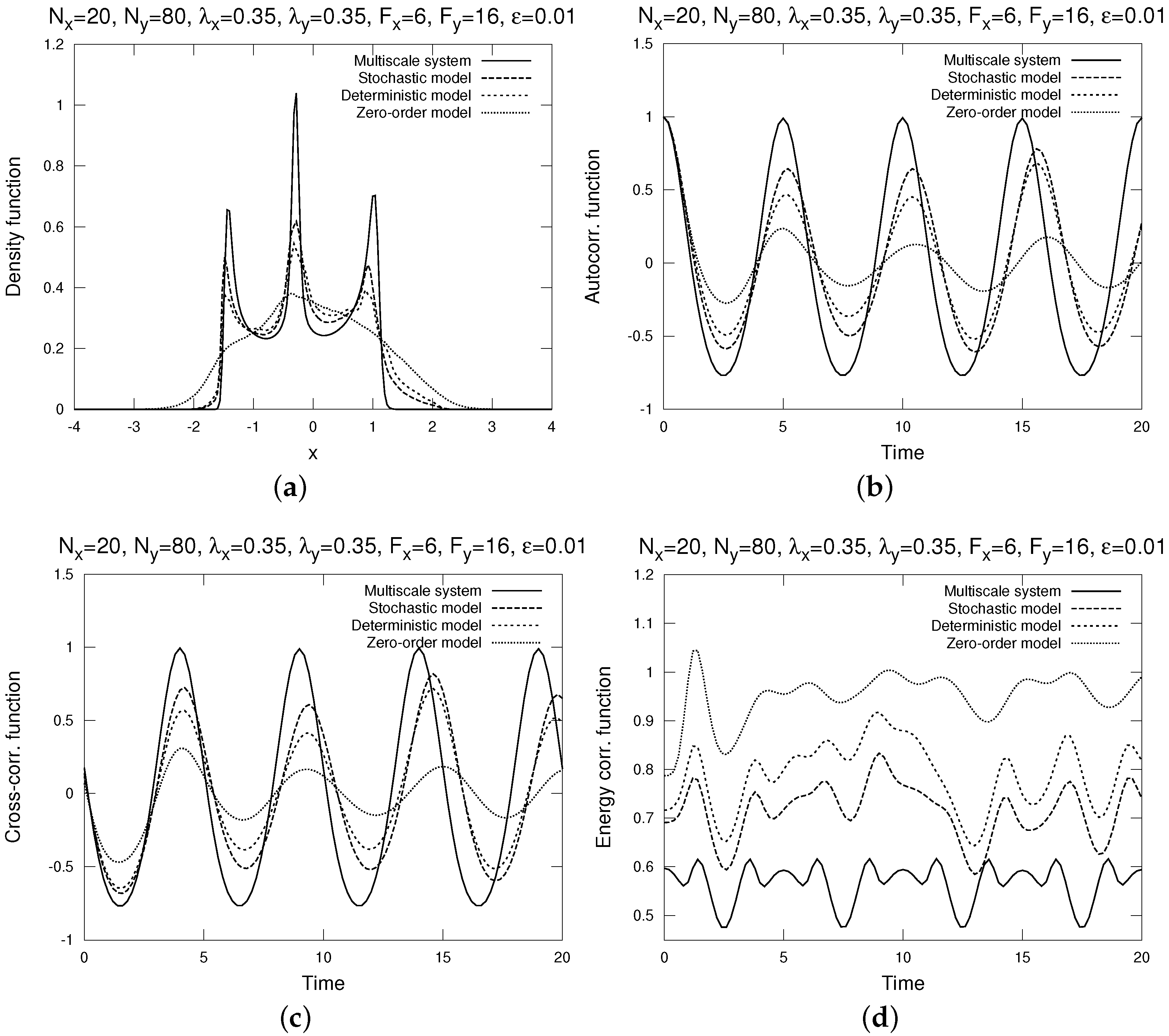
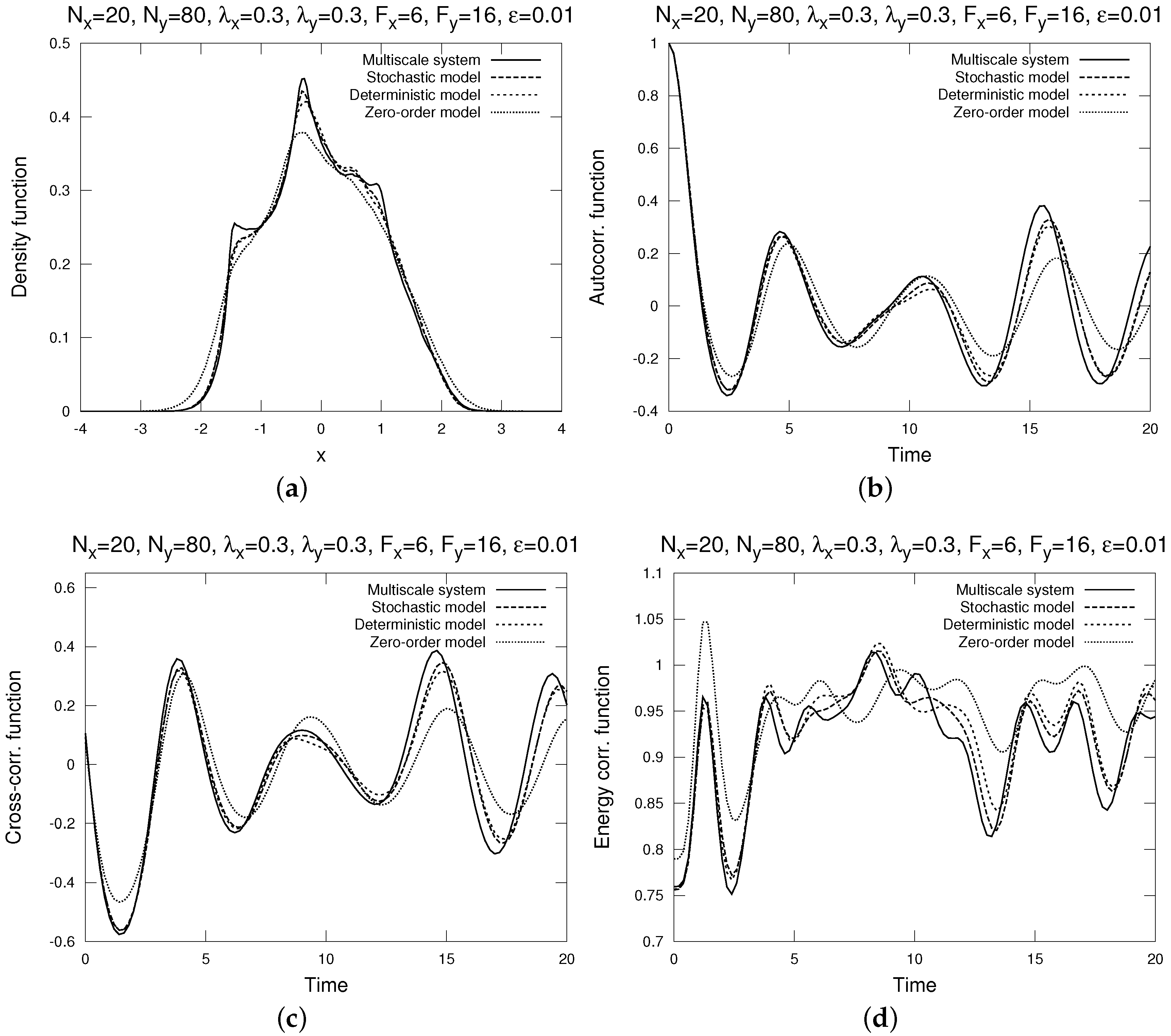
- The distribution density functions, computed by bin-counting. A distribution density function gives the best information about the one-point statistics of , as it shows the statistical distribution of in the phase space.
- The time auto-correlation functions , where the time average is over t, normalized by the variance (so that it always starts with 1).
- The time cross-correlation functions , also normalized by the variance .
- The energy auto-correlation functionThis energy auto-correlation function measures the non-Gaussianity of the process (it is identically 1 for all s if the process is Gaussian, such as the Ornstein-Uhlenbeck process). For details, see [23].
- , (so that ). Thus, the number of the fast variables is four times greater than the number of the slow variables.
- . The time scale separation of two orders of magnitude () is consistent with typical real-world geophysical processes (for example, the annual and diurnal cycles of the Earth’s atmosphere). Also, in large-scale atmospheric processes the time scale separation between slow and fast variables can be weaker than that (for example, typical time scale of equatorial Kelvin waves is about 70 days, and that of Yanai waves is about 30 days, which is well in between the annual and diurnal cycles), so we additionally test the dynamical regimes with weak time scale separation .
- . These values of coupling are chosen so that they are neither too weak, nor too strong (although 0.3 is weaker, and 0.35 is stronger). However, this small variation in coupling changes the dynamical regime in the slow variables between moderately () and weakly () chaotic and mixing, due to the suppression of chaos effect previously studied in [51].
- . The slow forcing adjusts the chaos and mixing properties of the slow variables, and in this work it is set to a weak-to-moderate chaotic regime . The reason for that is that it was found previously in [35] that in strongly chaotic and mixing regimes at slow variables there is not much of a difference between the multiscale dynamics and reduced models.
- . The fast forcing adjusts the chaos and mixing properties of the fast variables. Here the value of is chosen so that the fast variables are strongly chaotic and mixing for .
4.1. Moderate Mixing at Slow Variables With Weak Time Scale Separation


| Rel. Error | Stochastic | Deterministic | Zero-Order |
|---|---|---|---|
| Density | |||
| Corr. | |||
| Cross-corr. | |||
| Energy corr. |
4.2. Moderate Mixing at Slow Variables With Strong Time Scale Separation
| Rel. Error | Stochastic | Deterministic | Zero-Order |
|---|---|---|---|
| Density | |||
| Corr. | |||
| Cross-corr. | |||
| Energy corr. |
4.3. Weak Mixing at Slow Variables With Weak Time Scale Separation
| Rel. Error | Stochastic | Deterministic | Zero-Order |
|---|---|---|---|
| Density | |||
| Corr. | |||
| Cross-corr. | |||
| Energy corr. |
4.4. Weak Mixing at Slow Variables With Strong Time Scale Separation
| Rel. Error | Stochastic | Deterministic | Zero-Order |
|---|---|---|---|
| Density | |||
| Corr. | |||
| Cross-corr. | |||
| Energy corr. |

5. Conclusions
- In the situation where the deterministic reduced model was less chaotic and weaker mixing than the slow variables of the full multiscale dynamics, the stochastic model was more chaotic and stronger mixing, due to stochastic forcing smoothing out spikes in distribution density and introducing random decorrelation in time auto- and cross-correlation functions.
- In the situation where the deterministic reduced model was more chaotic and stronger mixing than the slow variables of the full multiscale dynamics, the stochastic model suppressed chaos and mixing in the reduced dynamics. While this effect seems somewhat counter-intuitive, it can be explained by the stochastic noise pushing the solution off the unstable manifold of the deterministic system (where the chaotic and mixing motion occurs) into the dissipative region around the system’s attractor, while not having enough random force to increase chaos and mixing on its own.
Acknowledgments
Conflicts of Interest
References
- Franzke, C.; Majda, A.; Vanden-Eijnden, E. Low-order stochastic model reduction for a realistic barotropic model climate. J. Atmos. Sci. 2005, 62, 1722–1745. [Google Scholar] [CrossRef]
- Hasselmann, K. Stochastic Climate Models: Part I. Theory. Tellus 1976, 28, 473–485. [Google Scholar] [CrossRef]
- Buizza, R.; Miller, M.; Palmer, T. Stochastic representation of model uncertainty in the ECMWF Ensemble Prediction System. Q. J. R. Meteor. Soc. 1999, 125, 2887–2908. [Google Scholar] [CrossRef]
- Palmer, T. A nonlinear dynamical perspective on model error: A proposal for nonlocal stochastic-dynamic parameterization in weather and climate prediction models. Q. J. R. Meteor. Soc. 2001, 127, 279–304. [Google Scholar] [CrossRef]
- Branstator, G.; Berner, J. Linear and nonlinear signatures in planetary wave dynamics of an AGCM: Phase space tendencies. J. Atmos. Sci. 2005, 62, 1792–1811. [Google Scholar] [CrossRef]
- Majda, A.; Franzke, C.; Crommelin, D. Normal forms for reduced stochastic climate models. Proc. Natl. Acad. Sci. USA 2009, 97, 12413–12417. [Google Scholar] [CrossRef] [PubMed]
- Kravtsov, S.; Kondrashov, D.; Ghil, M. Multilevel regression modeling of nonlinear processes: Derivation and applications to climatic variability. J. Clim. 2005, 18, 4404–4424. [Google Scholar] [CrossRef]
- Liu, D.; Vanden-Eijnden, E. Analysis of multiscale methods for stochastic differential equations. Commun. Pure Appl. Math. 2005, 58, 1544–1585. [Google Scholar]
- Fatkullin, I.; Vanden-Eijnden, E. A computational strategy for multiscale systems with applications to Lorenz 96 model. J. Comp. Phys. 2004, 200, 605–638. [Google Scholar] [CrossRef]
- Papanicolaou, G. Introduction to the Asymptotic Analysis of Stochastic Equations. Modern Modeling of Continuum Phenomena; Di Prima, R., Ed.; American Mathematical Society: Providence, RI, USA, 1977; Volume 16. [Google Scholar]
- Vanden-Eijnden, E. Numerical Techniques for multiscale dynamical systems with stochastic effects. Commun. Math. Sci. 2003, 1, 385–391. [Google Scholar] [CrossRef]
- Volosov, V. Averaging in systems of ordinary differential equations. Russ. Math. Surv. 1962, 17, 1–126. [Google Scholar] [CrossRef]
- Uhlenbeck, G.; Ornstein, L. On the theory of the Brownian motion. Phys. Rev. 1930, 36, 823–841. [Google Scholar] [CrossRef]
- Arnold, L.; Imkeller, P.; Wu, Y. Reduction of Deterministic Coupled Atmosphere-Ocean Models to Stochastic Ocean Models: A Numerical Case Study of the Lorenz-Maas System. Dyn. Syst. 2003, 18, 295–350. [Google Scholar] [CrossRef]
- Melbourne, I.; Stuart, A. A note on diffusion limits of chaotic skew product flows. Nonlinearity 2011, 24, 1361–1367. [Google Scholar] [CrossRef]
- Gottwald, G.; Melbourne, I. Homogenization for deterministic maps and multiplicative noise. Proc. R. Soc. 2013, A469, 20130201. [Google Scholar] [CrossRef]
- Kelly, D.; Melbourne, I. Deterministic Homogenization for Fast-Slow Systems with Chaotic Noise. Available online: http://xxx.lanl.gov/abs/1409.5748 (accessed on 18 December 2015).
- Kifer, Y. L2 Diffusion Approximation for Slow Motion in Averaging. Stoch. Dyn. 2003, 3, 213–246. [Google Scholar] [CrossRef]
- Crommelin, D.; Vanden-Eijnden, E. Subgrid scale parameterization with conditional Markov chains. J. Atmos. Sci. 2008, 65, 2661–2675. [Google Scholar] [CrossRef]
- Majda, A.; Timofeyev, I.; Vanden-Eijnden, E. Models for stochastic climate prediction. Proc. Natl. Acad. Sci. USA 1999, 96, 14687–14691. [Google Scholar] [CrossRef] [PubMed]
- Majda, A.; Timofeyev, I.; Vanden-Eijnden, E. Systematic strategies for stochastic mode reduction in climate. J. Atmos. Sci. 2003, 60, 1705–1722. [Google Scholar] [CrossRef]
- Majda, A.; Timofeyev, I.; Vanden-Eijnden, E. A Mathematical Framework for Stochastic Climate Models. Commun. Pure Appl. Math. 2001, 54, 891–974. [Google Scholar] [CrossRef]
- Majda, A.; Timofeyev, I.; Vanden-Eijnden, E. A priori Tests of a Stochastic Mode Reduction Strategy. Phys. D 2002, 170, 206–252. [Google Scholar] [CrossRef]
- Wilks, D. Effects of stochastic parameterizations in the Lorenz ’96 system. Q. J. R. Meteorol. Soc. 2005, 131, 389–407. [Google Scholar] [CrossRef]
- Katsoulakis, M.; Vlachos, G. Hierarchical kinetic Monte Carlo simulations for diffusion of interacting molecules. J. Chem. Phys. 2003, 112, 9412–9427. [Google Scholar] [CrossRef]
- Franzke, C.; Majda, A. Low-order stochastic mode reduction for a prototype atmospheric GCM. J. Atmos. Sci. 2006, 63, 457–479. [Google Scholar] [CrossRef]
- Branstator, G. Low-frequency patterns induced by stationary waves. J. Atmos. Sci. 1990, 47, 629–648. [Google Scholar] [CrossRef]
- Newman, M.; Sardeshmukh, P.; Penland, C. Stochastic forcing of the wintertime extratropical flow. J. Atmos. Sci. 1997, 54, 435–455. [Google Scholar] [CrossRef]
- Whitaker, J.; Sardeshmukh, P. A linear theory of extratropical synoptic eddy statistics. J. Atmos. Sci. 1998, 55, 237–258. [Google Scholar] [CrossRef]
- Zhang, Y.; Held, I. A linear stochastic model of a GCM’s midlatitude storm tracks. J. Atmos. Sci. 1999, 56, 3416–3435. [Google Scholar] [CrossRef]
- Majda, A.; Khouider, B. Stochastic and mesoscopic models for tropical convection. Proc. Natl. Acad. Sci. USA 2002, 99, 1123–1128. [Google Scholar] [CrossRef] [PubMed]
- Khouider, B.; Majda, A.; Katsoulakis, M. Coarse grained stochastic models for tropical convection. Proc. Natl. Acad. Sci. USA 2003, 100, 11941–11946. [Google Scholar] [CrossRef] [PubMed]
- Azencott, R.; Beri, A.; Timofeyev, I. Sub-sampling and Parametric Estimation for Multiscale Dynamics. Commun. Math. Sci. 2013, 11, 939–970. [Google Scholar] [CrossRef]
- Vannitsem, S. Stochastic Modelling and Predictability: Analysis of a Low-Order Coupled Ocean-Atmosphere Model. Phil. Trans. R. Soc. 2014, 372. [Google Scholar] [CrossRef] [PubMed]
- Abramov, R. A simple linear response closure approximation for slow dynamics of a multiscale system with linear coupling. Multiscale Model. Simul. 2012, 10, 28–47. [Google Scholar] [CrossRef]
- Abramov, R. A simple closure approximation for slow dynamics of a multiscale system: Nonlinear and multiplicative coupling. Multiscale Model. Simul. 2013, 11, 134–151. [Google Scholar] [CrossRef]
- Abramov, R. Short-time linear response with reduced-rank tangent map. Chin. Ann. Math. 2009, 30, 447–462. [Google Scholar] [CrossRef]
- Abramov, R. Approximate linear response for slow variables of deterministic or stochastic dynamics with time scale separation. J. Comput. Phys. 2010, 229, 7739–7746. [Google Scholar] [CrossRef]
- Abramov, R. Improved linear response for stochastically driven systems. Front. Math. China 2012, 7, 199–216. [Google Scholar] [CrossRef]
- Abramov, R.; Majda, A. New Approximations and Tests of Linear Fluctuation-Response for Chaotic Nonlinear Forced-Dissipative Dynamical Systems. J. Nonl. Sci. 2008, 18, 303–341. [Google Scholar] [CrossRef]
- Abramov, R.; Majda, A. Blended Response Algorithms for Linear Fluctuation-Dissipation for Complex Nonlinear Dynamical Systems. Nonlinearity 2007, 20, 2793–2821. [Google Scholar] [CrossRef]
- Abramov, R.; Majda, A. New algorithms for low frequency climate response. J. Atmos. Sci. 2009, 66, 286–309. [Google Scholar] [CrossRef]
- Majda, A.; Abramov, R.; Grote, M. Information Theory and Stochastics for Multiscale Nonlinear Systems. In CRM Monograph Series of Centre de Recherches Mathématiques, Université de Montréal; American Mathematical Society: Providence, RI, USA, 2005; Volume 25. [Google Scholar]
- Risken, H. The Fokker-Planck Equation, 2nd ed.; Springer-Verlag: New York, NY, USA, 1989. [Google Scholar]
- Lorenz, E. Predictability: A Problem Partly Solved. In Predictability of Weather and Climate; Palmer, T., Hagedom, R., Eds.; Cambridge University Press: England, UK, 1996. [Google Scholar]
- Lorenz, E.; Emanuel, K. Optimal Sites for Supplementary Weather Observations. J. Atmos. Sci. 1998, 55, 399–414. [Google Scholar] [CrossRef]
- Franzke, C. Dynamics of low-frequency variability: Barotropic mode. J. Atmos. Sci. 2002, 59, 2909–2897. [Google Scholar] [CrossRef]
- Selten, F. An efficient description of the dynamics of barotropic flow. J. Atmos. Sci. 1995, 52, 915–936. [Google Scholar] [CrossRef]
- Pavliotis, G.; Stuart, A. Multiscale Methods: Averaging and Homogenization; Springer: Berlin, Germany, 2008. [Google Scholar]
- Gikhman, I.; Skorokhod, A. Introduction to the Theory of Random Processes; Courier Dover Publications: Mineola, NY, USA, 1969. [Google Scholar]
- Abramov, R. Suppression of chaos at slow variables by rapidly mixing fast dynamics through linear energy-preserving coupling. Commun. Math. Sci. 2012, 10, 595–624. [Google Scholar] [CrossRef]
© 2015 by the authors; licensee MDPI, Basel, Switzerland. This article is an open access article distributed under the terms and conditions of the Creative Commons Attribution license ( http://creativecommons.org/licenses/by/4.0/).
Share and Cite
Abramov, R. A Simple Stochastic Parameterization for Reduced Models of Multiscale Dynamics. Fluids 2016, 1, 2. https://doi.org/10.3390/fluids1010002
Abramov R. A Simple Stochastic Parameterization for Reduced Models of Multiscale Dynamics. Fluids. 2016; 1(1):2. https://doi.org/10.3390/fluids1010002
Chicago/Turabian StyleAbramov, Rafail. 2016. "A Simple Stochastic Parameterization for Reduced Models of Multiscale Dynamics" Fluids 1, no. 1: 2. https://doi.org/10.3390/fluids1010002
APA StyleAbramov, R. (2016). A Simple Stochastic Parameterization for Reduced Models of Multiscale Dynamics. Fluids, 1(1), 2. https://doi.org/10.3390/fluids1010002