Author Contributions
Conceptualization, H.C., J.L., T.L. and M.Z.; methodology, H.C. and J.L.; software, H.C. and J.L.; validation, H.C., J.L., H.X. and M.H.; formal analysis, H.C., J.L., H.X. and M.H.; investigation, H.C. and J.L.; resources, T.L., M.Z. and H.X.; data curation, H.C. and J.L.; writing—original draft preparation, H.C. and J.L.; writing—review and editing, T.L. and M.Z.; visualization, H.C. and J.L.; supervision, T.L. and M.Z.; project administration, T.L. and M.Z.; funding acquisition, T.L. and M.Z. All authors have read and agreed to the published version of the manuscript.
Figure 1.
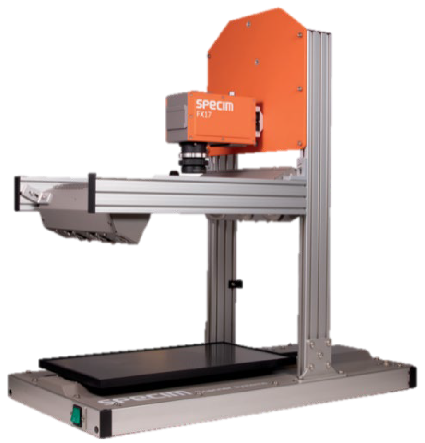
Specim FX17 hyperspectral camera and scanning platform used for tuber image acquisition. The orange camera housing is mounted above the scanning stage.
Figure 1.
Specim FX17 hyperspectral camera and scanning platform used for tuber image acquisition. The orange camera housing is mounted above the scanning stage.
Figure 2.
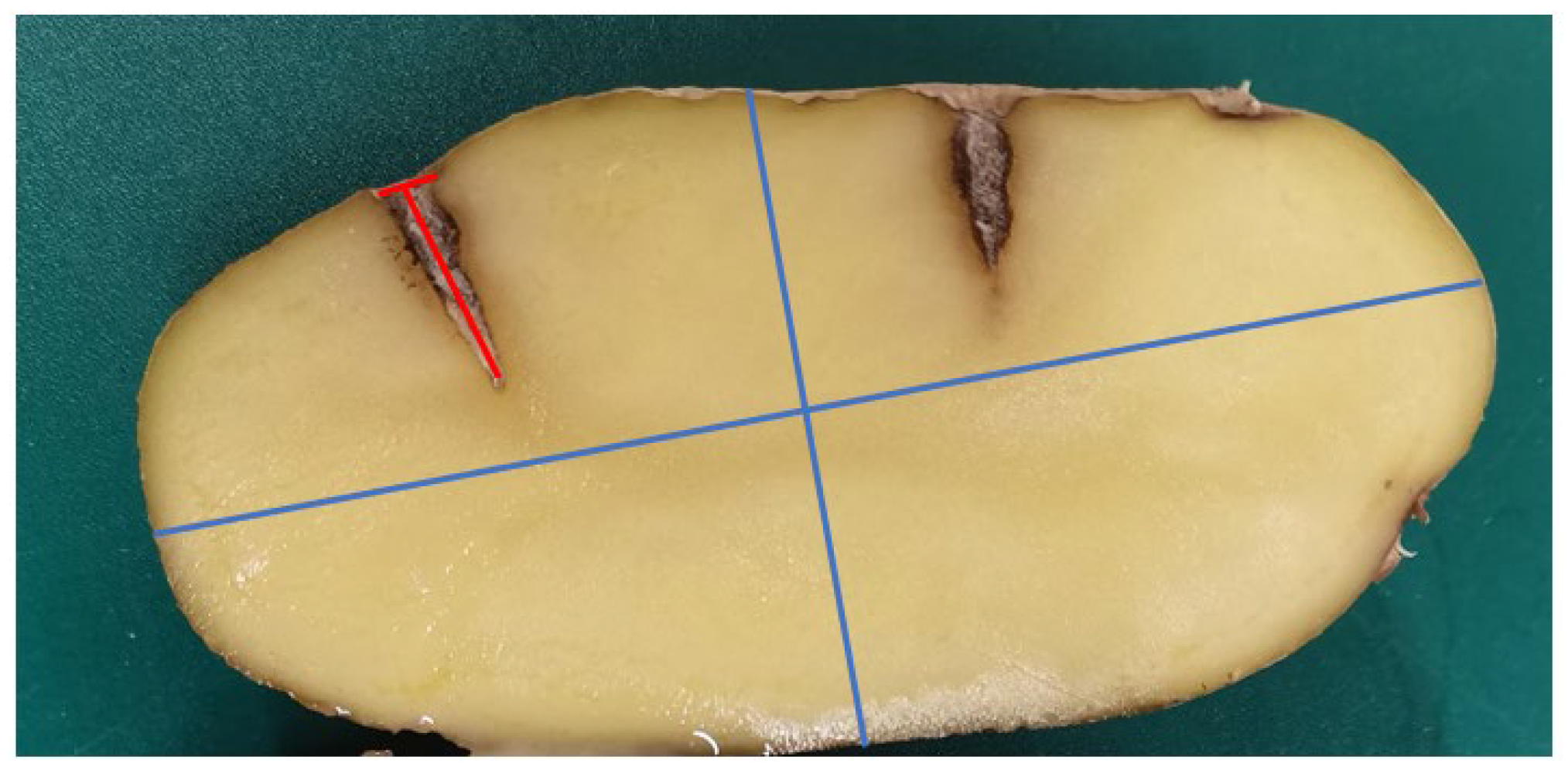
Measurement of tuber and lesion dimensions on a cut surface. Blue lines mark the principal tuber dimensions visible in the section, and red lines mark the lesion radius and depth. Tuber length, width, and thickness were used for the ellipsoidal volume estimate. Effective lesion depth was calculated by subtracting the approximately 3 mm inoculation hole depth from the measured lesion depth.
Figure 2.
Measurement of tuber and lesion dimensions on a cut surface. Blue lines mark the principal tuber dimensions visible in the section, and red lines mark the lesion radius and depth. Tuber length, width, and thickness were used for the ellipsoidal volume estimate. Effective lesion depth was calculated by subtracting the approximately 3 mm inoculation hole depth from the measured lesion depth.
Figure 3.
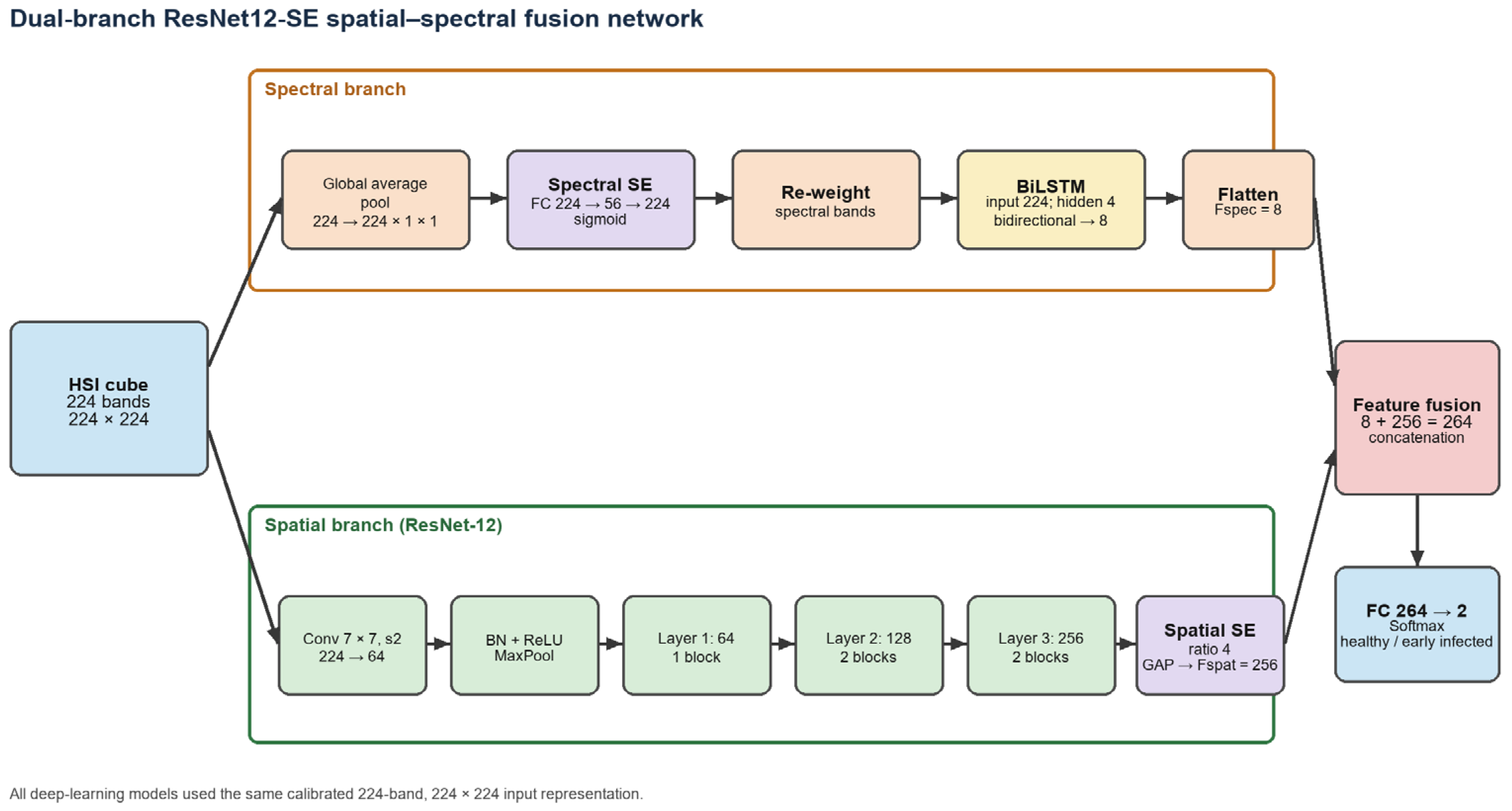
Architecture of the proposed dual-branch ResNet12-SE network. The input is a calibrated 224-band, 224 × 224 hyperspectral cube. The orange and green outlines identify the spectral and spatial branches, respectively; purple boxes denote SE modules, the yellow box denotes BiLSTM, and the pink box denotes feature fusion. The spatial branch produces Fspat = 256 and the spectral branch produces Fspec = 8, yielding 264 features before binary classification. HSI, hyperspectral imaging; SE, squeeze-and-excitation; BiLSTM, bidirectional long short-term memory; FC, fully connected; GAP, global average pooling; BN, batch normalization; ReLU, rectified linear unit.
Figure 3.
Architecture of the proposed dual-branch ResNet12-SE network. The input is a calibrated 224-band, 224 × 224 hyperspectral cube. The orange and green outlines identify the spectral and spatial branches, respectively; purple boxes denote SE modules, the yellow box denotes BiLSTM, and the pink box denotes feature fusion. The spatial branch produces Fspat = 256 and the spectral branch produces Fspec = 8, yielding 264 features before binary classification. HSI, hyperspectral imaging; SE, squeeze-and-excitation; BiLSTM, bidirectional long short-term memory; FC, fully connected; GAP, global average pooling; BN, batch normalization; ReLU, rectified linear unit.
Figure 4.
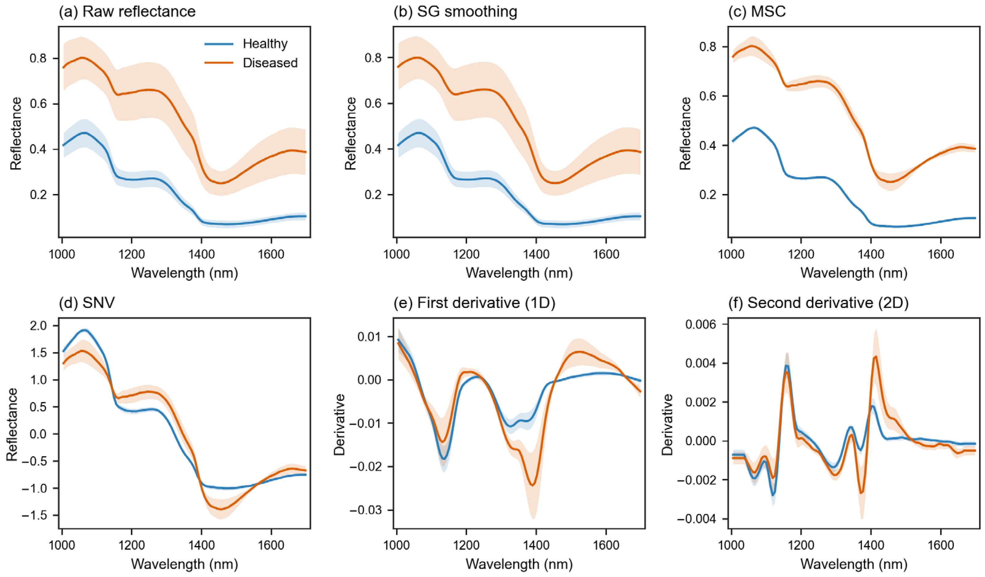
Mean spectra of healthy and early-infected records: (a) raw reflectance; (b) SG smoothing; (c) MSC; (d) SNV; (e) first derivative (1D); and (f) second derivative (2D). Blue and orange curves represent healthy and early-infected records, respectively; shaded bands represent the standard deviation across records. SG, Savitzky–Golay smoothing; MSC, multiplicative scatter correction; SNV, standard normal variate.
Figure 4.
Mean spectra of healthy and early-infected records: (a) raw reflectance; (b) SG smoothing; (c) MSC; (d) SNV; (e) first derivative (1D); and (f) second derivative (2D). Blue and orange curves represent healthy and early-infected records, respectively; shaded bands represent the standard deviation across records. SG, Savitzky–Golay smoothing; MSC, multiplicative scatter correction; SNV, standard normal variate.
Figure 5.
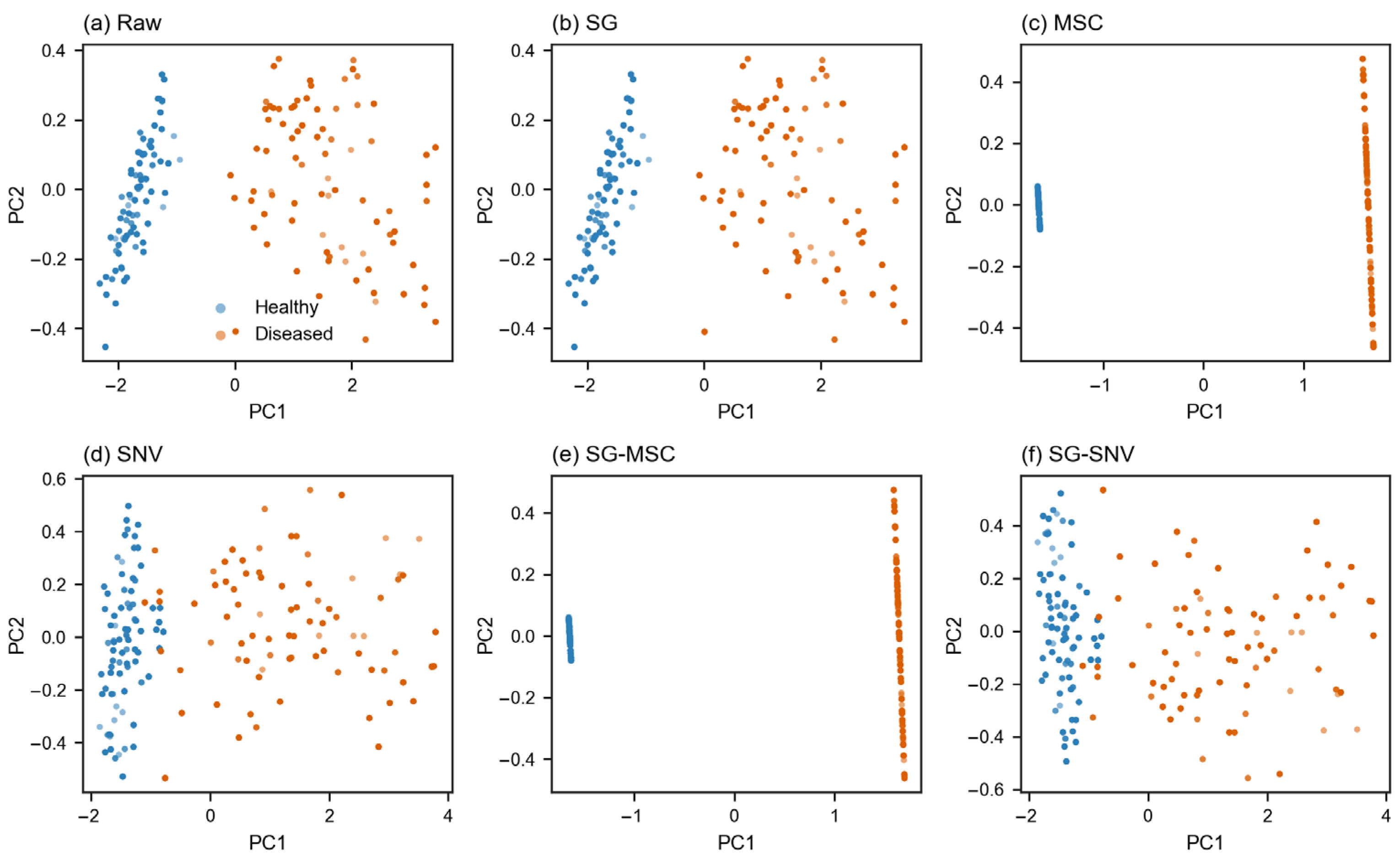
Two-dimensional PCA projections of healthy and early-infected records: (a) raw spectra; (b) SG; (c) MSC; (d) SNV; (e) SG-MSC; and (f) SG-SNV. Blue and orange points represent healthy and early-infected records, respectively. PC1 and PC2 denote the first and second principal components. PCA, principal component analysis; SG, Savitzky–Golay smoothing; MSC, multiplicative scatter correction; SNV, standard normal variate.
Figure 5.
Two-dimensional PCA projections of healthy and early-infected records: (a) raw spectra; (b) SG; (c) MSC; (d) SNV; (e) SG-MSC; and (f) SG-SNV. Blue and orange points represent healthy and early-infected records, respectively. PC1 and PC2 denote the first and second principal components. PCA, principal component analysis; SG, Savitzky–Golay smoothing; MSC, multiplicative scatter correction; SNV, standard normal variate.
Figure 6.
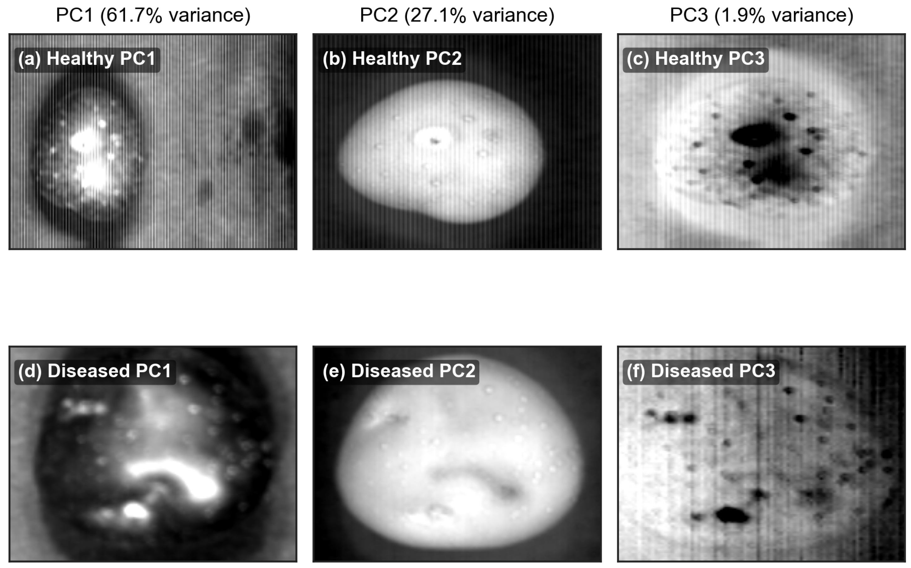
Representative principal component images: (a–c) PC1, PC2, and PC3 of a healthy tuber, respectively; (d–f) PC1, PC2, and PC3 of an early-infected tuber, respectively. The first three components explain 61.7%, 27.1%, and 1.9% of the variance, respectively. PC, principal component; PCA, principal component analysis.
Figure 6.
Representative principal component images: (a–c) PC1, PC2, and PC3 of a healthy tuber, respectively; (d–f) PC1, PC2, and PC3 of an early-infected tuber, respectively. The first three components explain 61.7%, 27.1%, and 1.9% of the variance, respectively. PC, principal component; PCA, principal component analysis.
Figure 7.
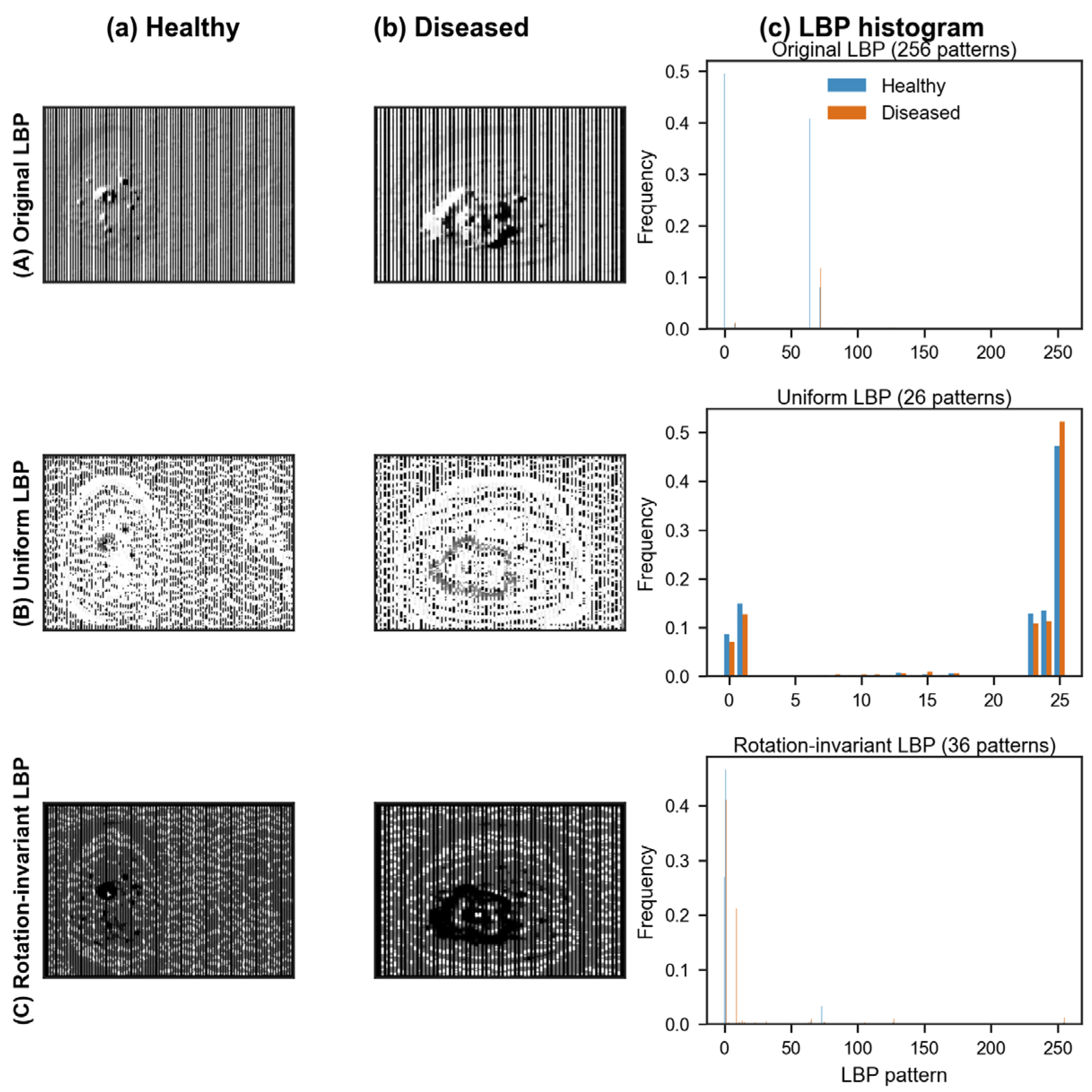
LBP feature maps and histograms for representative healthy and early-infected records. (A) Original LBP; (B) uniform LBP; (C) rotation-invariant LBP; (a) healthy; (b) early infected; (c) pattern frequency histogram. LBP, local binary pattern.
Figure 7.
LBP feature maps and histograms for representative healthy and early-infected records. (A) Original LBP; (B) uniform LBP; (C) rotation-invariant LBP; (a) healthy; (b) early infected; (c) pattern frequency histogram. LBP, local binary pattern.
Figure 8.
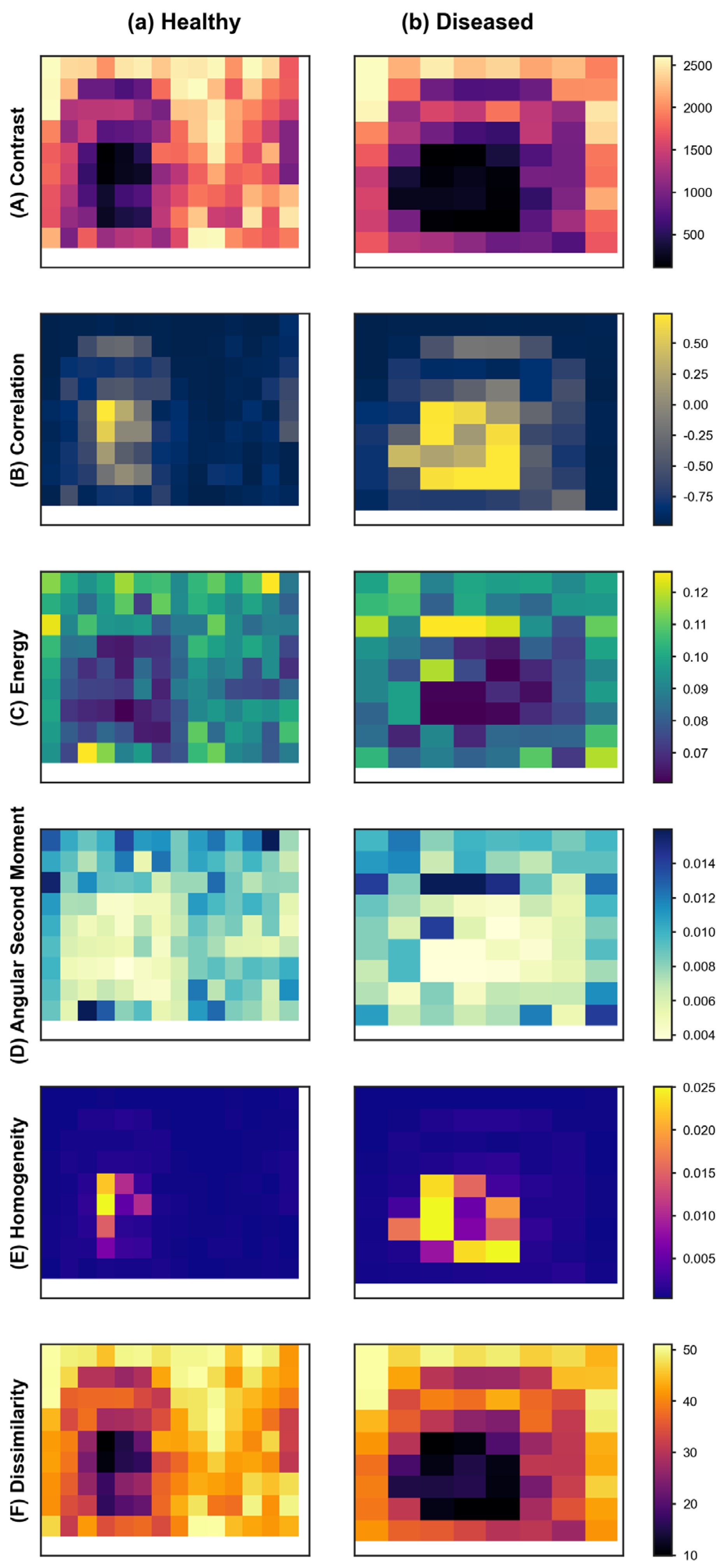
GLCM feature maps for representative tubers: column (a), healthy; column (b), early infected. Rows show (A) contrast, (B) correlation, (C) energy, (D) angular second moment, (E) homogeneity, and (F) dissimilarity. Color bars indicate the local value of each descriptor. GLCM, gray-level co-occurrence matrix.
Figure 8.
GLCM feature maps for representative tubers: column (a), healthy; column (b), early infected. Rows show (A) contrast, (B) correlation, (C) energy, (D) angular second moment, (E) homogeneity, and (F) dissimilarity. Color bars indicate the local value of each descriptor. GLCM, gray-level co-occurrence matrix.
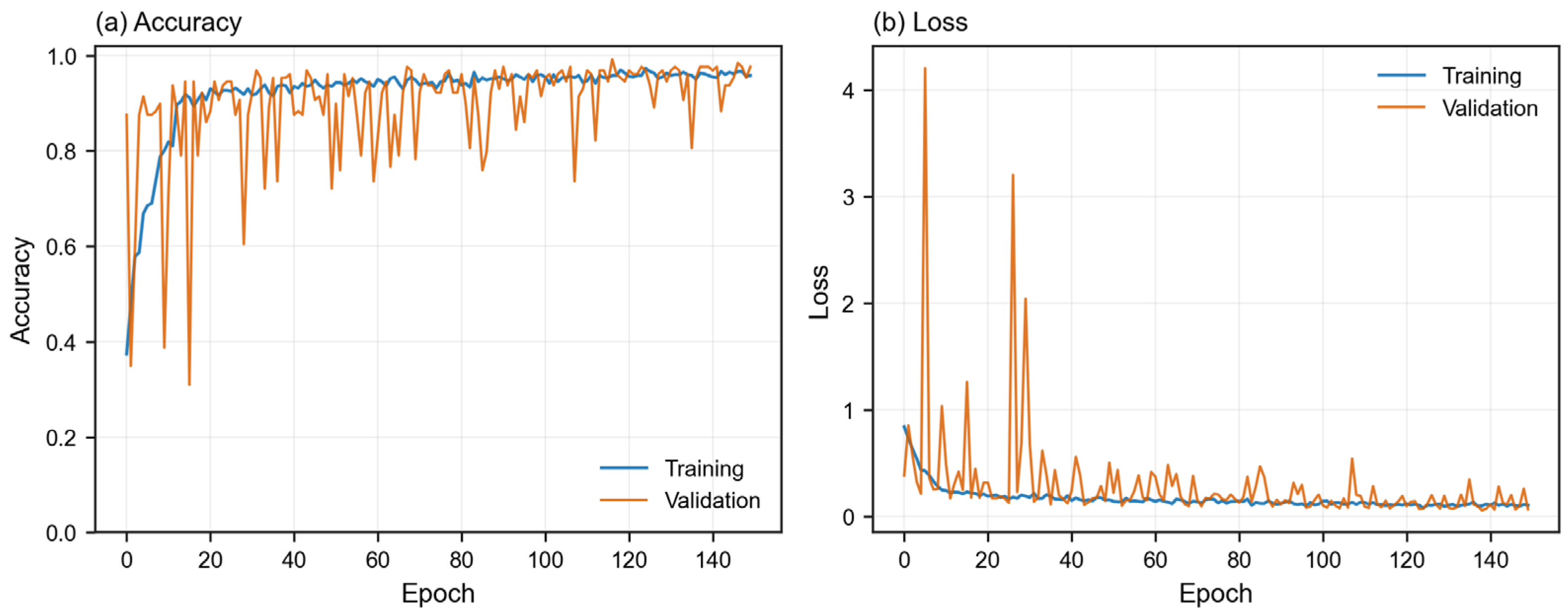
Figure 9.
Training and validation curves of the proposed ResNet12-SE model: (a) accuracy; (b) loss. Blue and orange curves represent the training and validation sets, respectively.
Figure 9.
Training and validation curves of the proposed ResNet12-SE model: (a) accuracy; (b) loss. Blue and orange curves represent the training and validation sets, respectively.
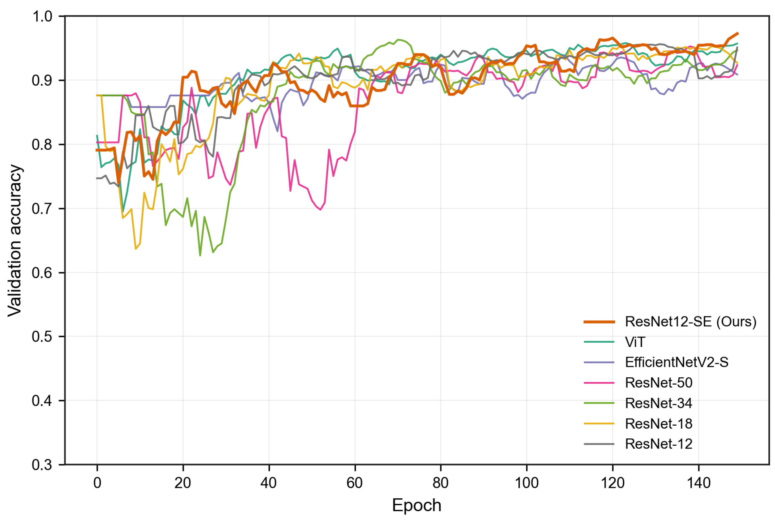
Figure 10.
Validation accuracy curves of different deep learning models. Curves show the recorded trajectory for the fixed data split; they are not repeated-run confidence bands.
Figure 10.
Validation accuracy curves of different deep learning models. Curves show the recorded trajectory for the fixed data split; they are not repeated-run confidence bands.
Table 1.
Single-split full-spectrum SVM accuracy under different preprocessing methods. SG, Savitzky–Golay smoothing; MSC, multiplicative scatter correction; SNV, standard normal variate; 1D, first derivative; 2D, second derivative.
Table 1.
Single-split full-spectrum SVM accuracy under different preprocessing methods. SG, Savitzky–Golay smoothing; MSC, multiplicative scatter correction; SNV, standard normal variate; 1D, first derivative; 2D, second derivative.
| Preprocessing Method | SG | 2D | 1D | SNV | MSC | SG-2D | SG-1D | SG-SNV | SG-MSC |
|---|
| Accuracy (%) | 93 | 92 | 88 | 58 | 91 | 90 | 94 | 94 | 97 |
Table 2.
Representative global GLCM descriptors calculated from the displayed PC1 images. The values are descriptive image-level measurements and not group-level estimates. GLCM, gray-level co-occurrence matrix; ASM, angular second moment.
Table 2.
Representative global GLCM descriptors calculated from the displayed PC1 images. The values are descriptive image-level measurements and not group-level estimates. GLCM, gray-level co-occurrence matrix; ASM, angular second moment.
| Representative PC1 Image | Contrast | Correlation | Energy | Homogeneity | Dissimilarity | Angular Second Moment |
|---|
| Healthy | 73.5762 | 0.0938 | 0.1384 | 0.0142 | 8.5373 | 0.0191 |
| Early infected | 59.6150 | 0.4225 | 0.1473 | 0.0182 | 7.6687 | 0.0216 |
Table 3.
Single-split accuracy of conventional models using selected spectral features. CARS, competitive adaptive reweighted sampling; SPA, successive projections algorithm; SVM, support vector machine; KNN, K-nearest neighbor; RF, random forest; BP, backpropagation neural network.
Table 3.
Single-split accuracy of conventional models using selected spectral features. CARS, competitive adaptive reweighted sampling; SPA, successive projections algorithm; SVM, support vector machine; KNN, K-nearest neighbor; RF, random forest; BP, backpropagation neural network.
| Feature–Classifier | CARS-RF | SPA-SVM | CARS-SVM | SPA-KNN |
|---|
| Accuracy (%) | 89.45 | 93.95 | 94.17 | 95.68 |
Table 4.
Single-split accuracy benchmarks for models using LBP, GLCM, and fused LBP–GLCM texture features. Values are percentages rounded to two decimal places. LBP, local binary pattern; GLCM, gray-level co-occurrence matrix.
Table 4.
Single-split accuracy benchmarks for models using LBP, GLCM, and fused LBP–GLCM texture features. Values are percentages rounded to two decimal places. LBP, local binary pattern; GLCM, gray-level co-occurrence matrix.
| Classifier | Feature Set | Accuracy (%) |
|---|
| SVM | LBP | 87.71 |
| GLCM | 83.26 |
| KNN | LBP | 74.92 |
| GLCM | 82.82 |
| RF | LBP | 86.15 |
| GLCM | 84.01 |
| BP | LBP | 77.09 |
| GLCM | 70.04 |
| SVM | LBP–GLCM | 91.13 |
Table 5.
Single-run ablation accuracies for the ResNet12-SE model under the fixed data split. A check mark (✓) indicates that a module was included, and a cross (×) indicates that it was omitted. SE, squeeze-and-excitation; LSTM, long short-term memory.
Table 5.
Single-run ablation accuracies for the ResNet12-SE model under the fixed data split. A check mark (✓) indicates that a module was included, and a cross (×) indicates that it was omitted. SE, squeeze-and-excitation; LSTM, long short-term memory.
| ResNet-12 | Spatial SE | Bidirectional LSTM | Spectral SE | Single-Run Accuracy (%) |
|---|
| ✓ | × | × | × | 90.67 |
| ✓ | ✓ | × | × | 92.24 |
| ✓ | × | ✓ | × | 93.79 |
| ✓ | ✓ | ✓ | × | 94.57 |
| ✓ | × | ✓ | ✓ | 95.34 |
| ✓ | ✓ | ✓ | ✓ | 98.22 |
Table 6.
Single-split test accuracy of deep learning models using the common calibrated 224-band input.
Table 6.
Single-split test accuracy of deep learning models using the common calibrated 224-band input.
| Model | Single-Split Test Accuracy (%) | Model | Single-Split Test Accuracy (%) |
|---|
| ResNet-18 | 92.72 | ResNet-50 | 93.79 |
| ResNet-34 | 94.89 | EfficientNetV2-S | 94.73 |
| ResNet12-SE | 98.22 | ViT | 97.43 |