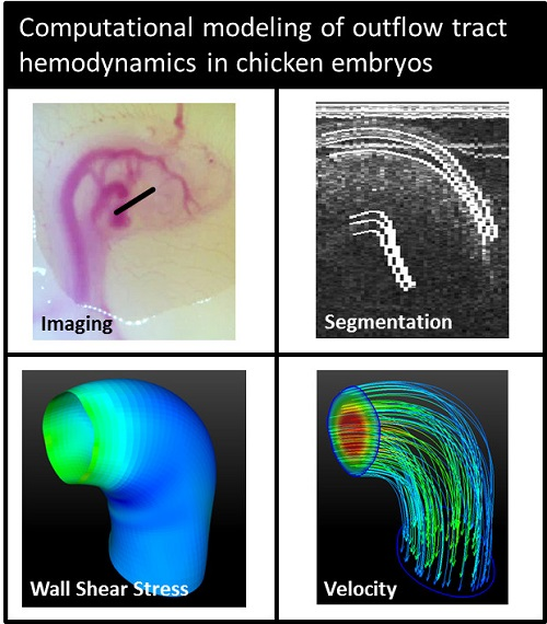
4-D Computational Modeling of Cardiac Outflow Tract Hemodynamics over Looping Developmental Stages in Chicken Embryos


Abstract

1. Introduction
2. Materials and Methods
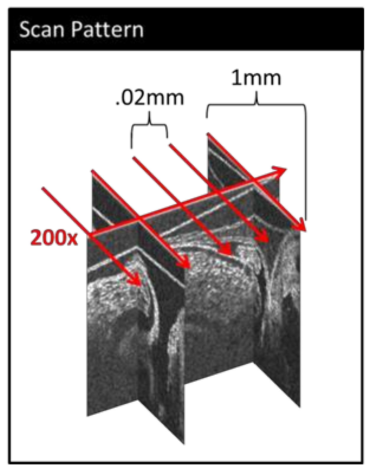
2.1. Imaging
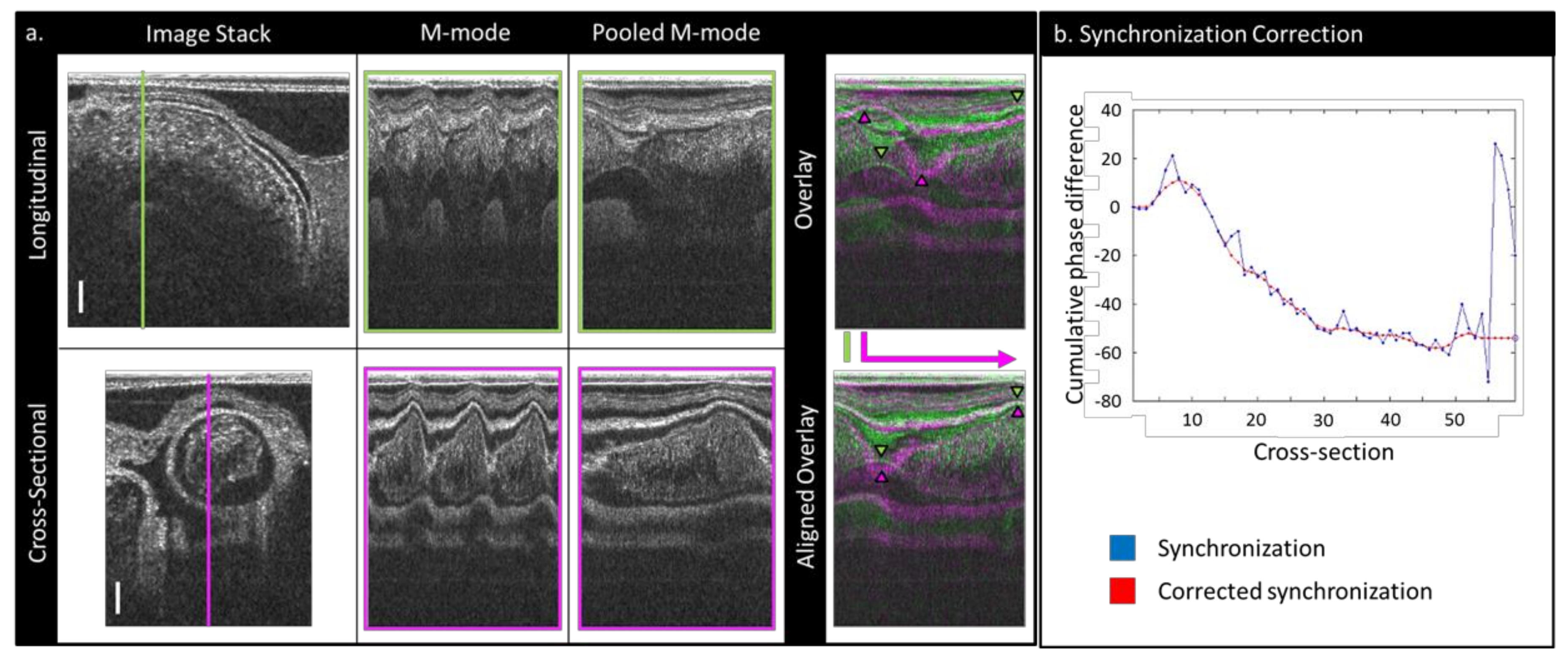
2.2. Image Post-Processing
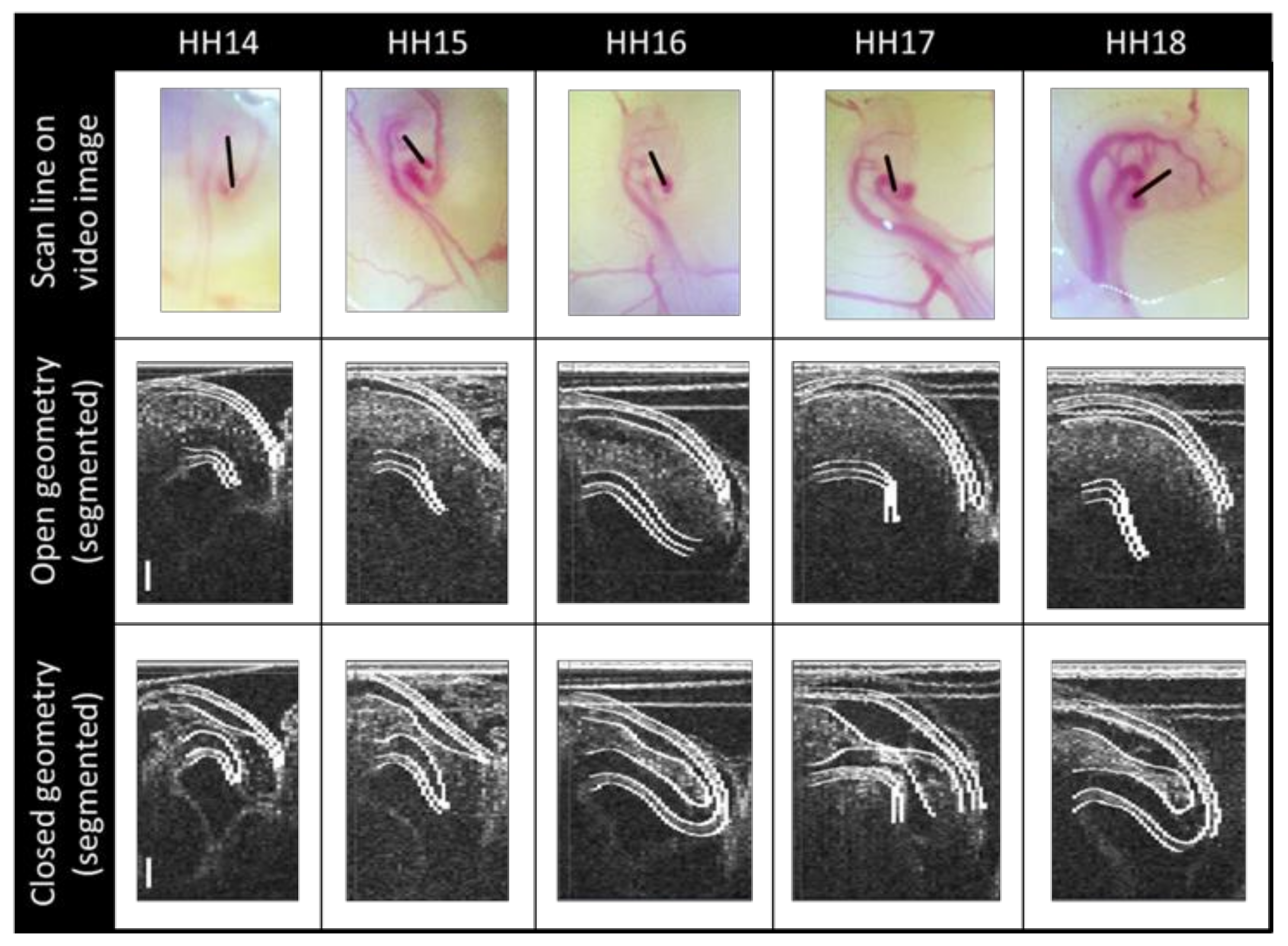
2.3. Segmenting
2.4. Computational Fluid Dynamics Simulations
2.5. Geometrical Assessment and Stress Analysis
2.6. Embryonic Sex Determination
3. Results
3.1. Physiology and Geometry
3.2. CFD
4. Discussion
Supplementary Materials
Author Contributions
Funding
Acknowledgments
Conflicts of Interest
References
- Hoffman, J.I.E.; Kaplan, S. The incidence of congenital heart disease. J. Am. Coll. Cardiol. 2002, 39, 1890–1900. [Google Scholar] [CrossRef]
- Reller, M.D.; Strickland, M.J.; Riehle-Colarusso, T.; Mahle, W.T.; Correa, A. Prevalence of congenital heart defects in metropolitan Atlanta, 1998–2005. J. Pediatr. 2008, 153, 807–813. [Google Scholar] [CrossRef] [PubMed]
- Oster, M.E.; Lee, K.A.; Honein, M.A.; Riehle-Colarusso, T.; Shin, M.; Correa, A. Temporal trends in survival among infants with critical congenital heart defects. Pediatrics 2013, 131, e1502–e1508. [Google Scholar] [CrossRef] [PubMed]
- Russo, C.A.; Elixhauser, A. Hospitalizations for Birth Defects, 2004; U.S. Agency for Healthcare Research and Quality: Rockville, MD, USA, 2007. [Google Scholar]
- Petrini, J.; Broussard, C.; Gilboa, S.; Lee, K.; Oster, M.; Honein, M. Racial Differences by Gestational age in Neonatal Deaths Attributable to Congenital Heart Defects-United States, 2003–2006; Centers for Disease Control and Prevention: Atlanta, GA, USA, 2010; pp. 1208–1211. [Google Scholar]
- Hartman, R.J.; Rasmussen, S.A.; Botto, L.D.; Riehle-Colarusso, T.; Martin, C.L.; Cragan, J.D.; Shin, M.; Correa, A. The contribution of chromosomal abnormalities to congenital heart defects: A population-based study. Pediatr. Cardiol. 2011, 32, 1147–1157. [Google Scholar] [CrossRef] [PubMed]
- Courchaine, K.; Rykiel, G.; Rugonyi, S. Influence of blood flow on cardiac development. Prog. Biophys. Mol. Biol. 2018, 137, 95–110. [Google Scholar] [CrossRef] [PubMed]
- Lucitti, J.L.; Jones, E.A.; Huang, C.; Chen, J.; Fraser, S.E.; Dickinson, M.E. Vascular remodeling of the mouse yolk sac requires hemodynamic force. Development 2007, 134, 3317–3326. [Google Scholar] [CrossRef] [PubMed]
- Menon, V.; Eberth, J.F.; Goodwin, R.L.; Potts, J.D. Altered hemodynamics in the embryonic heart affects outflow valve development. J. Cardiovasc. Dev. Dis. 2015, 2, 108–124. [Google Scholar] [CrossRef] [PubMed]
- Broekhuizen, M.L.A.; Hogers, B.; DeRuiter, M.C.; Poelmann, R.E.; Gittenberger-De Groot, A.C.; Wladimiroff, J.W. Altered hemodynamics in chick embryos after extraembryonic venous obstruction. Ultrasound Obstet. Gynecol. 1999, 13, 437–445. [Google Scholar] [CrossRef] [PubMed]
- Stekelenburg-de Vos, S.; Steendijk, P.; Ursem, N.T.C.; Wladimiroff, J.W.; Poelmann, R.E. Systolic and diastolic ventricular function in the normal and extra-embryonic venous clipped chicken embryo of stage 24: A pressure–volume loop assessment. Ultrasound Obstet. Gynecol. 2007, 30, 325–331. [Google Scholar] [CrossRef] [PubMed]
- Midgett, M.; Rugonyi, S. Congenital heart malformations induced by hemodynamic altering surgical interventions. Front. Physiol. 2014, 5, 287. [Google Scholar] [CrossRef] [PubMed]
- Midgett, M.; Thornburg, K.; Rugonyi, S. Blood flow patterns underlie developmental heart defects. Am. J. Physiol. Heart Circ. Physiol. 2017, 312, H632–H642. [Google Scholar] [CrossRef] [PubMed]
- Hove, J.R.; Koster, R.W.; Forouhar, A.S.; Acevedo-Bolton, G.; Fraser, S.E.; Gharib, M. Intracardiac fluid forces are an essential epigenetic factor for embryonic cardiogenesis. Nature 2003, 421, 170–172. [Google Scholar] [CrossRef] [PubMed]
- Fishman, N.H.; Hof, R.B.; Rudolph, A.M.; Heymann, M.A. Models of congenital heart disease in fetal lambs. Circulation 1978, 58, 354–364. [Google Scholar] [CrossRef] [PubMed]
- Kimimasa, T.; Garrison, J.B.; Liu, L.J.; Tinney, J.P.; Keller, B.B. Three-dimensional myofiber architecture of the embryonic left ventricle during normal development and altered mechanical loads. Anat. Rec. Part A: Discov. Mol. Cell. Evol. Biol. 2005, 283A, 193–201. [Google Scholar]
- Midgett, M.; López, C.S.; David, L.; Maloyan, A.; Rugonyi, S. Increased hemodynamic load in early embryonic stages alters endocardial to mesenchymal transition. Front. Physiol. 2017, 8, 56. [Google Scholar] [CrossRef] [PubMed]
- Waldo, K.L.; Kumiski, D.H.; Wallis, K.T.; Stadt, H.A.; Hutson, M.R.; Platt, D.H.; Kirby, M.L. Conotruncal myocardium arises from a secondary heart field. Development 2001, 128, 3179–3188. [Google Scholar] [PubMed]
- Dyer, L.A.; Kirby, M.L. The role of secondary heart field in cardiac development. Dev. Biol. 2009, 336, 137–144. [Google Scholar] [CrossRef] [PubMed]
- Midgett, M.; Chivukula, V.K.; Dorn, C.; Wallace, S.; Rugonyi, S. Blood flow through the embryonic heart outflow tract during cardiac looping in HH13-HH18 chicken embryos. J. R. Soc. Interface 2015, 12, 20150652. [Google Scholar] [CrossRef] [PubMed]
- Stovall, S.; Midgett, M.; Thornburg, K.; Rugonyi, S. Changes in dynamic embryonic heart wall motion in response to outflow tract banding measured using video densitometry. J. Biomed. Opt. 2016, 21, 116003. [Google Scholar] [CrossRef] [PubMed]
- Carson, J.P.; Rennie, M.Y.; Danilchik, M.; Thornburg, K.; Rugonyi, S. A chicken embryo cardiac outflow tract atlas for registering changes due to abnormal blood flow. In Proceedings of the 38th IEEE Engineering in Medicine and Biology Society. Annual Conference, Orlando, FL, USA, 17–20 August 2016; pp. 1236–1239. [Google Scholar]
- Bharadwaj, K.N.; Spitz, C.; Shekhar, A.; Yalcin, H.C.; Butcher, J.T. Computational fluid dynamics of developing avian outflow tract heart valves. Ann. Biomed. Eng. 2012, 40, 2212–2227. [Google Scholar] [CrossRef] [PubMed]
- Poelma, C.; Van der Heiden, K.; Hierck, B.P.; Poelmann, R.E.; Westerweel, J. Measurements of the wall shear stress distribution in the outflow tract of an embryonic chicken heart. J. R. Soc. Interface 2010, 7, 91–103. [Google Scholar] [CrossRef] [PubMed]
- Oosterbaan, A.M.; Ursem, N.T.; Struijk, P.C.; Bosch, J.G.; van der Steen, A.F.; Steegers, E.A. Doppler flow velocity waveforms in the embryonic chicken heart at developmental stages corresponding to 5-8 weeks of human gestation. Ultrasound Obstet. Gynecol. 2009, 33, 638–644. [Google Scholar] [CrossRef] [PubMed]
- Liu, A.; Nickerson, A.; Troyer, A.; Yin, X.; Cary, R.; Thornburg, K.; Wang, R.; Rugonyi, S. Quantifying blood flow and wall shear stresses in the outflow tract of chick embryonic hearts. Comput. Struct. 2011, 89, 855–867. [Google Scholar] [CrossRef] [PubMed]
- Liu, A.; Yin, X.; Shi, L.; Li, P.; Thornburg, K.L.; Wang, R.; Rugonyi, S. Biomechanics of the chick embryonic heart outflow tract at HH18 using 4D optical coherence tomography imaging and computational modeling. PLoS ONE 2012, 7, e40869. [Google Scholar] [CrossRef] [PubMed]
- Hamburger, V.; Hamilton, H.L. A series of normal stages in the development of the chick embryo. Dev. Dyn. 1992, 195, 231–272. [Google Scholar] [CrossRef] [PubMed]
- Goenezen, S.; Chivukula, V.K.; Midgett, M.; Phan, L.; Rugonyi, S. 4D subject-specific inverse modeling of the chick embryonic heart outflow tract hemodynamics. Biomech. Modeling Mechanobiol. 2016, 15, 723–743. [Google Scholar] [CrossRef] [PubMed]
- Liu, A.; Wang, R.K.; Thornburg, K.L.; Rugonyi, S. Efficient postacquisition synchronization of 4-D nongated cardiac images obtained from optical coherence tomography: Application to 4-D reconstruction of the chick embryonic heart. J. Biomedical Opt. 2009, 14, 044020. [Google Scholar] [CrossRef] [PubMed]
- Yin, X.; Liu, A.; Thornburg, K.L.; Wang, R.K.; Rugonyi, S. Extracting cardiac shapes and motion of the chick embryo heart outflow tract from four-dimensional optical coherence tomography images. J. Biomed. Opt. 2012, 17, 096005. [Google Scholar] [CrossRef] [PubMed]
- Yalcin, H.C.; Shekhar, A.; McQuinn, T.C.; Butcher, J.T. Hemodynamic patterning of the avian atrioventricular valve. Dev. Dyn. Off. Publ. Am. Assoc. Anat. 2011, 240, 23–35. [Google Scholar] [CrossRef] [PubMed]
- Jordan, C.D.; Flood, J.G.; Laposata, M.; Lewandrowski, K.B. Normal reference laboratory values. N. Engl. J. Med. 1992, 327, 718–724. [Google Scholar]
- Vedula, V.; Lee, J.; Xu, H.; Kuo, C.C.J.; Hsiai, T.K.; Marsden, A.L. A method to quantify mechanobiologic forces during zebrafish cardiac development using 4-d light sheet imaging and computational modeling. PLoS Comput. Biol. 2017, 13, e1005828. [Google Scholar] [CrossRef] [PubMed]
- Fridolfsson, A.K.; Cheng, H.; Copeland, N.G.; Jenkins, N.A.; Liu, H.C.; Raudsepp, T.; Woodage, T.; Chowdhary, B.; Halverson, J.; Ellegren, H. Evolution of the avian sex chromosomes from an ancestral pair of autosomes. Proc. Natl. Acad. Sci. USA 1998, 95, 8147–8152. [Google Scholar] [CrossRef] [PubMed]
- Liu, W.-Y.; Zhao, C.-J.; Li, J.-Y. A non-invasive and inexpensive PCR-based procedure for rapid sex diagnosis of chinese gamecock chicks and embryos. J. Anim. Vet. Adv. 2010, 9, 962–970. [Google Scholar] [CrossRef]
- Hu, N.; Clark, E.B. Hemodynamics of the stage 12 to stage 29 chick embryo. Circ. Res. 1989, 65, 1665–1670. [Google Scholar] [CrossRef] [PubMed]
- Hogers, B.; DeRuiter, M.C.; Gittenberger-de Groot, A.C.; Poelmann, R.E. Unilateral vitelline vein ligation alters intracardiac blood flow patterns and morphogenesis in the chick embryo. Circ. Res. 1997, 80, 473–481. [Google Scholar] [CrossRef] [PubMed]


| HH14 | HH15 | HH16 | HH17 | HH18 | |
|---|---|---|---|---|---|
| (n = 3) | (n = 1) | (n = 4) | (n = 4) | (n = 4) | |
| # Male | 2 | 0 | 3 | 2 | 1 |
| Cardiac cycle (ms) | 486 ± 54 | 507 | 408 ± 35 | 410 ± 30 | 400 ± 35 |
| Maximum lumen volume (mm3) | 03 ± 005 | 04 | 07 ± 02 | 095 ± 02 | 09 ± 02 |
| Mean lumen volume (mm3) | 02 ± 0.004 | 02 | 04 ± 01 | 05 ± 01 | 05 ± 01 |
| Centerline length (mm) | 54 ± 01 | 59 | 73 ± 07 | 78 ± 12 | 69 ± 0.08 |
| Maximum WSS (Pa) | 6.3 ± 7 | 6.3 | 11.0 ± 5.5 | 10.6 ± 2 | 7.9 ± 3.4 |
| Mean WSS (Pa) | 1.1 ± 5 | 97 | 1.1 ± 22 | 9 ± 0.17 | 75 ± 0.20 |
| Mean oscillatory shear index (OSI) | 25 ± 11 | 31 | 29 ± 03 | 21 ± 0.12 | 16 ± 0.13 |
| Maximum OSI | 45 ± 08 | 49 | 49 ± 01 | 38 ± 0.16 | 3 ± 0.22 |
| Maximum backflow velocity (mm/s) | 30 ± 19 | 40 | 50 ± 6 | 30 ± 12 | 21 ± 11 |
| Maximum forward velocity (mm/s) | 43 ± 12 | 35 | 82 ± 29 | 90 ± 15 | 62 ± 6 |
| Backflow volume (mm3/beat) | 02 ± 02 | 04 | 04 ± 002 | 04 ± 0.02 | 02 ± 0.02 |
| Forward volume (mm3/beat) | 07 ± 02 | 1 | 15 ± 02 | 25 ± 0.11 | 21 ± 0.02 |
| Stroke volume (mm3/beat) | 05 ± 01 | 06 | 12 ± 02 | 21 ± 0.1 | 19 ± 0.03 |
| Cardiac efficiency | 75 ± 19 | 64 | 76 ± 02 | 84 ± 0.1 | 92 ± 0.08 |
| Maximum flow rate (mm3/s) | 72 ± 6 | 87 | 1.7 ± 0.21 | 2.8 ± 1.24 | 2.4 ± 0.17 |
© 2019 by the authors. Licensee MDPI, Basel, Switzerland. This article is an open access article distributed under the terms and conditions of the Creative Commons Attribution (CC BY) license (http://creativecommons.org/licenses/by/4.0/).
Share and Cite
Courchaine, K.; Gray, M.J.; Beel, K.; Thornburg, K.; Rugonyi, S. 4-D Computational Modeling of Cardiac Outflow Tract Hemodynamics over Looping Developmental Stages in Chicken Embryos. J. Cardiovasc. Dev. Dis. 2019, 6, 11. https://doi.org/10.3390/jcdd6010011
Courchaine K, Gray MJ, Beel K, Thornburg K, Rugonyi S. 4-D Computational Modeling of Cardiac Outflow Tract Hemodynamics over Looping Developmental Stages in Chicken Embryos. Journal of Cardiovascular Development and Disease. 2019; 6(1):11. https://doi.org/10.3390/jcdd6010011
Chicago/Turabian StyleCourchaine, Katherine, MacKenzie J. Gray, Kaitlin Beel, Kent Thornburg, and Sandra Rugonyi. 2019. "4-D Computational Modeling of Cardiac Outflow Tract Hemodynamics over Looping Developmental Stages in Chicken Embryos" Journal of Cardiovascular Development and Disease 6, no. 1: 11. https://doi.org/10.3390/jcdd6010011
APA StyleCourchaine, K., Gray, M. J., Beel, K., Thornburg, K., & Rugonyi, S. (2019). 4-D Computational Modeling of Cardiac Outflow Tract Hemodynamics over Looping Developmental Stages in Chicken Embryos. Journal of Cardiovascular Development and Disease, 6(1), 11. https://doi.org/10.3390/jcdd6010011