
A New Odd Beta Prime-Burr X Distribution with Applications to Petroleum Rock Sample Data and COVID-19 Mortality Rate

 ,
,  and
and
Abstract
1. Introduction
- 1.
- for
- 2.
- is differentiable and monotonically non-decreasing.
- 3.
- as but as
- (i)
- to improve the general performance of the classical Burr X distribution, which can handle skewed and heavy-tailed data sets when compared to other competitive models;
- (ii)
- to improve a model kurtosis that is more flexible in contrast to the referenced models;
- (iii)
- to develop a model with different shapes, such as left-skewed, right-skewed, re versed-J, and symmetric;
- (iv)
- to introduce a new model with various hazard functions that can capture increasing, decreasing, bathtub, and concave-convex shapes; and
- (v)
- to consistently offer superior fit in comparison to well-established, generated distributions for the same baseline distribution.
2. Overview of the Previous Studies
- 1.
- pioneering the use of the extended Burr X distribution for modelling geological data, a discipline that had not previously been investigated within this framework;
- 2.
- introducing a new Burr X distribution version developed to offer a good fit for petroleum rock samples and COVID-19 data sets; and
- 3.
- applying the new distribution to different kinds of data, because the three shape parameters can control the tail of data.

| Year | Model | Application | Authors |
|---|---|---|---|
| 2023 | Odd beta prime Burr X distribution | Geological and COVID-19 data | New |
| Unit–power Burr X distribution | COVID-19 data | [63] | |
| Exponentiated beta Burr X distribution | Failure time data | [64] | |
| Maxwell Burr X distribution | COVID-19 data | [44] | |
| Kavya–Manoharan Burr X distribution | Survival, waiting time, and financial data | [25] | |
| Exponentiated Kavya–Manoharan Burr X model | Medical and survival data | [65] | |
| 2022 | Exponentiated Weibull Burr X distribution | Survival data | [41] |
| Gamma odd Burr X Weibull distribution | Taxes revenue and repair time data | [66] | |
| Type I half-logistic Burr X Weibull distribution | COVID-19 data | [67] | |
| Burr X logistic exponential distribution | Engineering and physics data | [68] | |
| Kumaraswamy Burr X distribution | Physics, engineering, and medical data | [43] | |
| Generalized Burr X Lomax distribution | Failure time | [69] | |
| Sine-exponentiated Weibull Burr X distribution | Food chain, wholesale, and physics data | [42] | |
| 2021 | Exponentiated Burr X distribution | Physics data | [40] |
| Transmuted Burr X exponential distribution | Physics and failure time data | [70] | |
| Truncated Burr X exponential distribution | Actuarial and financial data | [71] | |
| Odd log-logistic Burr-X normal distribution | Agricultural and medical data | [72] | |
| Type I half-logistic Burr X Lomax distribution | COVID-19 data | [73] | |
| Type I half-logistic Burr X exponential distribution | COVID-19 data | [73] | |
| Type I half-logistic Burr X Rayleigh distribution | COVID-19 data | [73] | |
| 2020 | Transmuted Burr X distribution | Reliability data | [39] |
| Power Burr X distribution | Physics and hydrological data | [38] | |
| Poisson Burr X inverse Rayleigh distribution | Physics and engineering data | [74] | |
| Odd Burr–Burr X distribution | Failure time, medical, survival, and physics data | [75] | |
| 2019 | Odd log-logistic Burr X distribution | Reliability data | [76] |
| Type I half-logistic Burr X distribution | Physics data | [37] | |
| Burr X Fréchet distribution | Survival data | [77] | |
| Zero truncated Poisson Burr X Weibull distribution | Reliability and medical data | [78] | |
| Poisson Burr X Weibull distribution | Failure time and survival data | [79] | |
| Burr X exponentiated exponential distribution | Physics data | [80] | |
| Burr X exponentiated Weibull distribution | Failure time and survival data | [81] | |
| Burr X Nadarajah Haghighi distribution | Hydrological data | [82] | |
| Marshall–Olkin exponentiated Burr X distribution | Physics data | [83] | |
| 2018 | Exponentiated generalized Burr X distribution | Physics data | [84] |
| Burr X exponentiated exponential distribution | Failure time and survival data | [85] | |
| Burr X Lomax distribution | Survival data | [86] | |
| Beta Kumaraswamy Burr X distribution | Physics and medical data | [87] | |
| 2017 | Weibull Burr X distribution | Reliability data | [88] |
| Burr X Lomax distribution | Medical data | [32] | |
| Burr X Pareto distribution | Financial time series data | [89] | |
| Burr X exponentiated Fréchet distribution | Survival and hydrological data | [90] | |
| Marshall–Olkin extended Burr X distribution | Physics data | [91] | |
| Marshall–Olkin Burr X Lomax distribution | Physics, hydrological, and survival data | [36] | |
| Weibull Burr X distribution | Hydrological and failure time data | [35] | |
| 2016 | Gamma Burr X distribution | Failure data | [34] |
| Beta Burr X distribution | Physics data | [92] |
3. Development of Odd Beta Prime-Burr X Distribution
Linear Representations
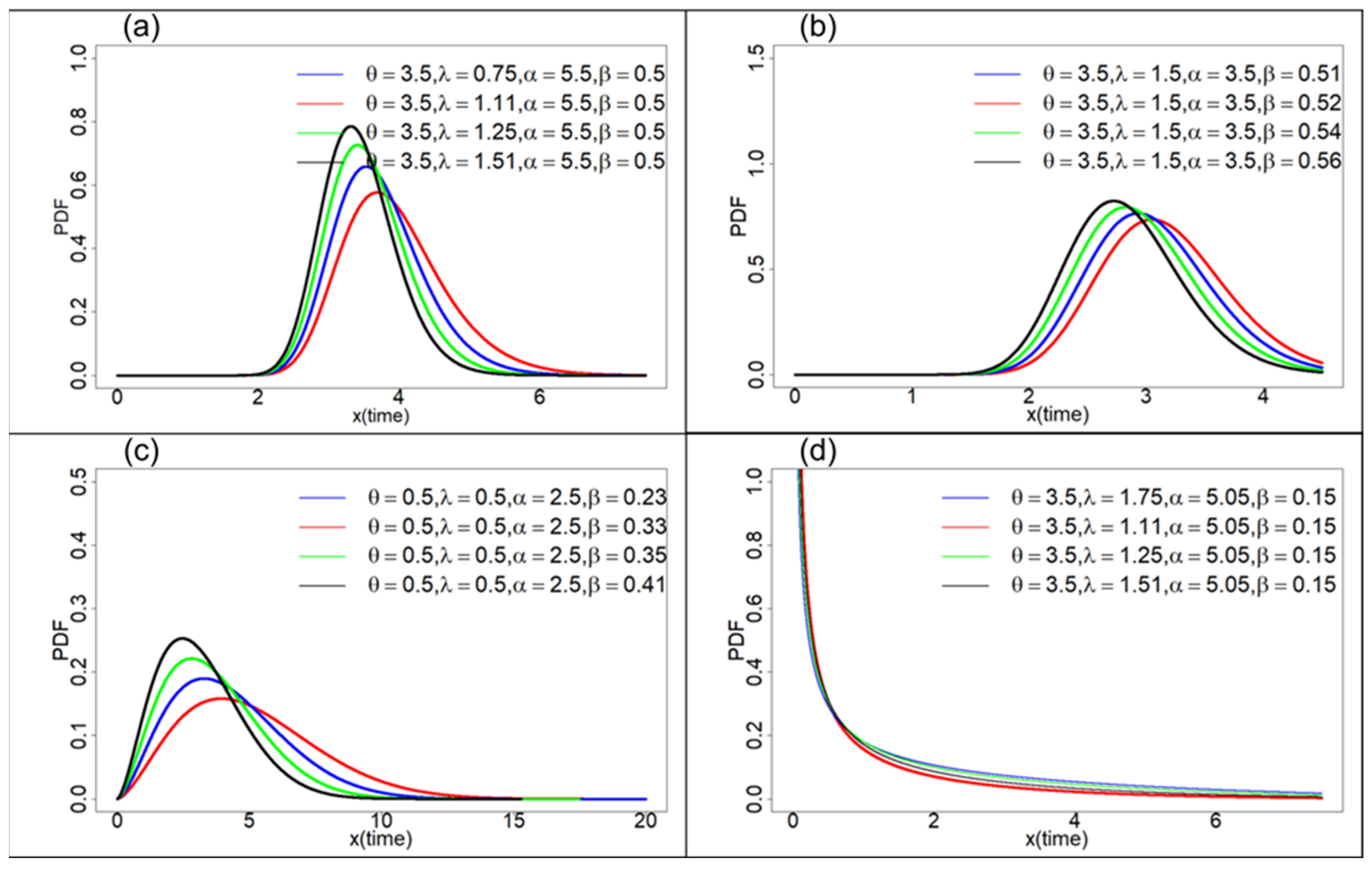
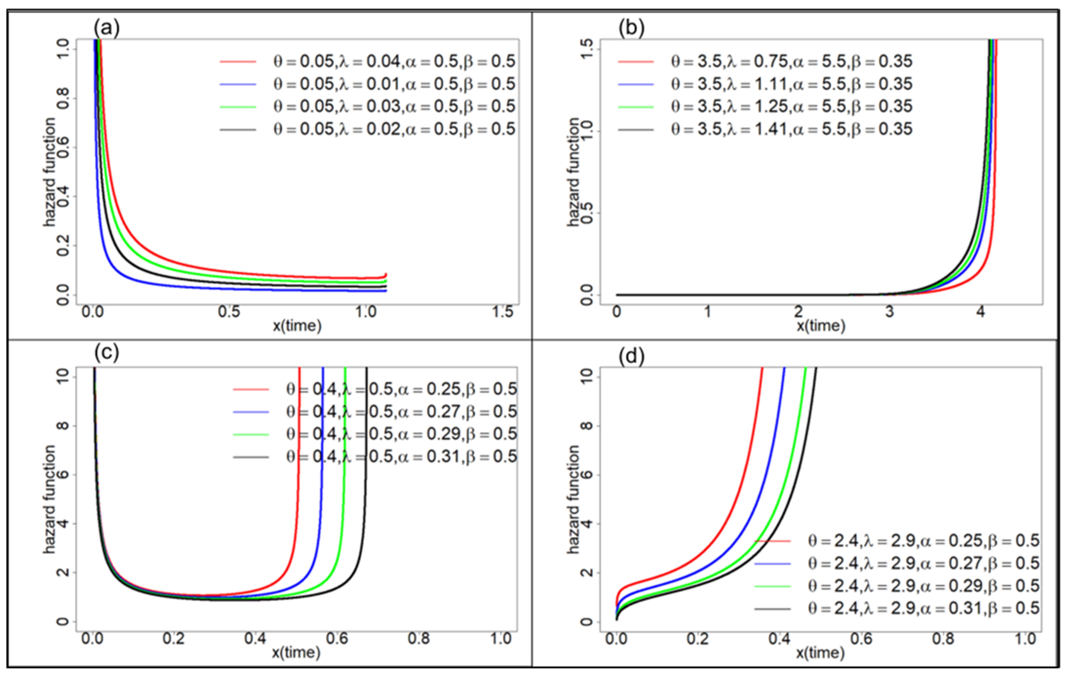
4. Statistical Features
4.1. Moments
4.2. Moment-Generating Function
4.3. Rényi and q Entropies
- (i)
- Rényi entropy
- (ii)
- q-entropy
4.4. Quantile Function
4.5. Quantile Based on Bowley’s Skewness and Moor’s Kurtosis
4.6. Limit Behavior
5. Parameter Estimation
Maximum-Likelihood Function
6. Monte Carlo Simulation Study
| Algorithm 1. Algorithm of Monte Carlo simulation for various sample sizes and selected parameter values. |
Case I: . Case II: .
Bias and MSE , where .
|
7. Applications to Petroleum Rock Samples and COVID-19 Mortality Rates
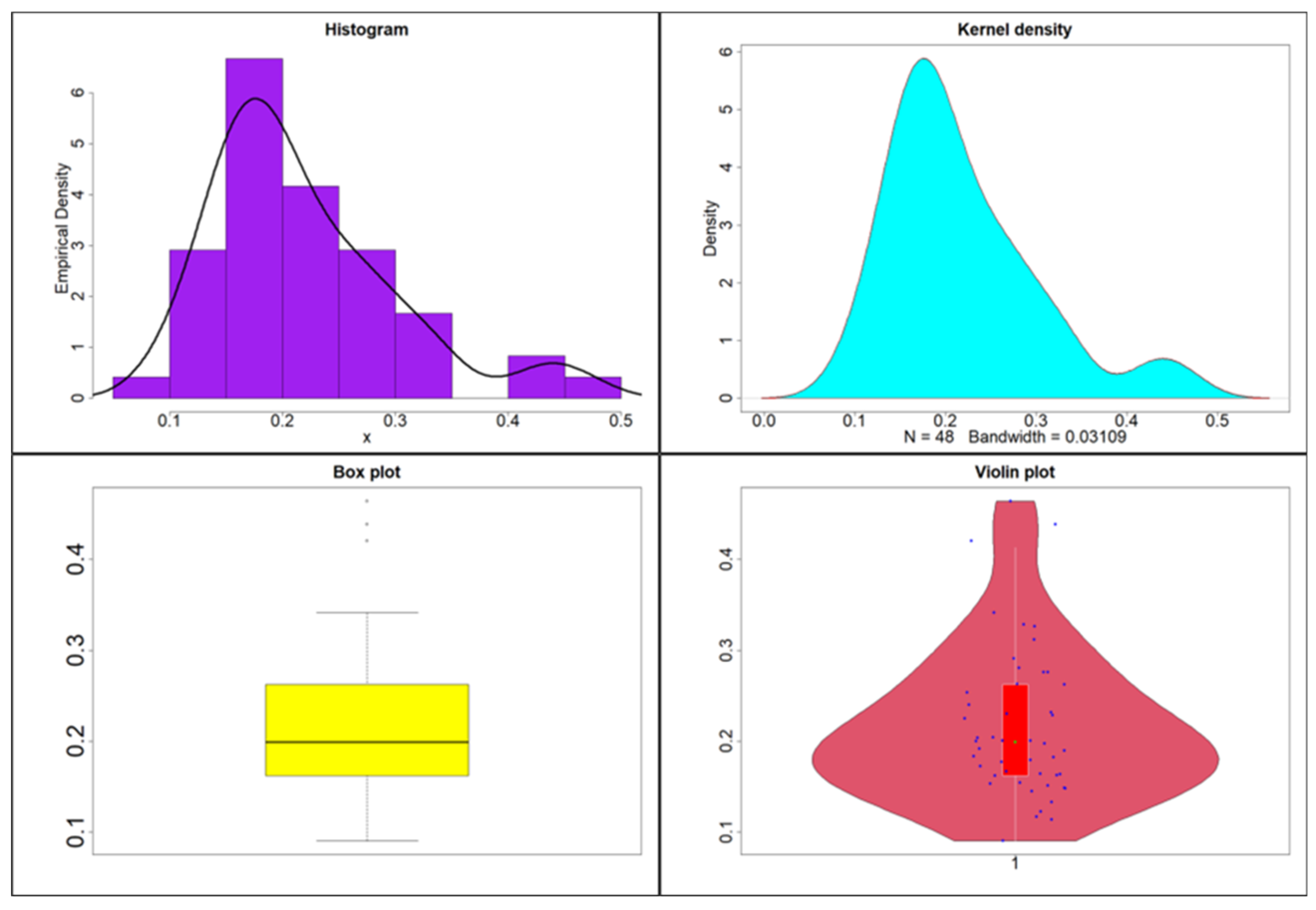
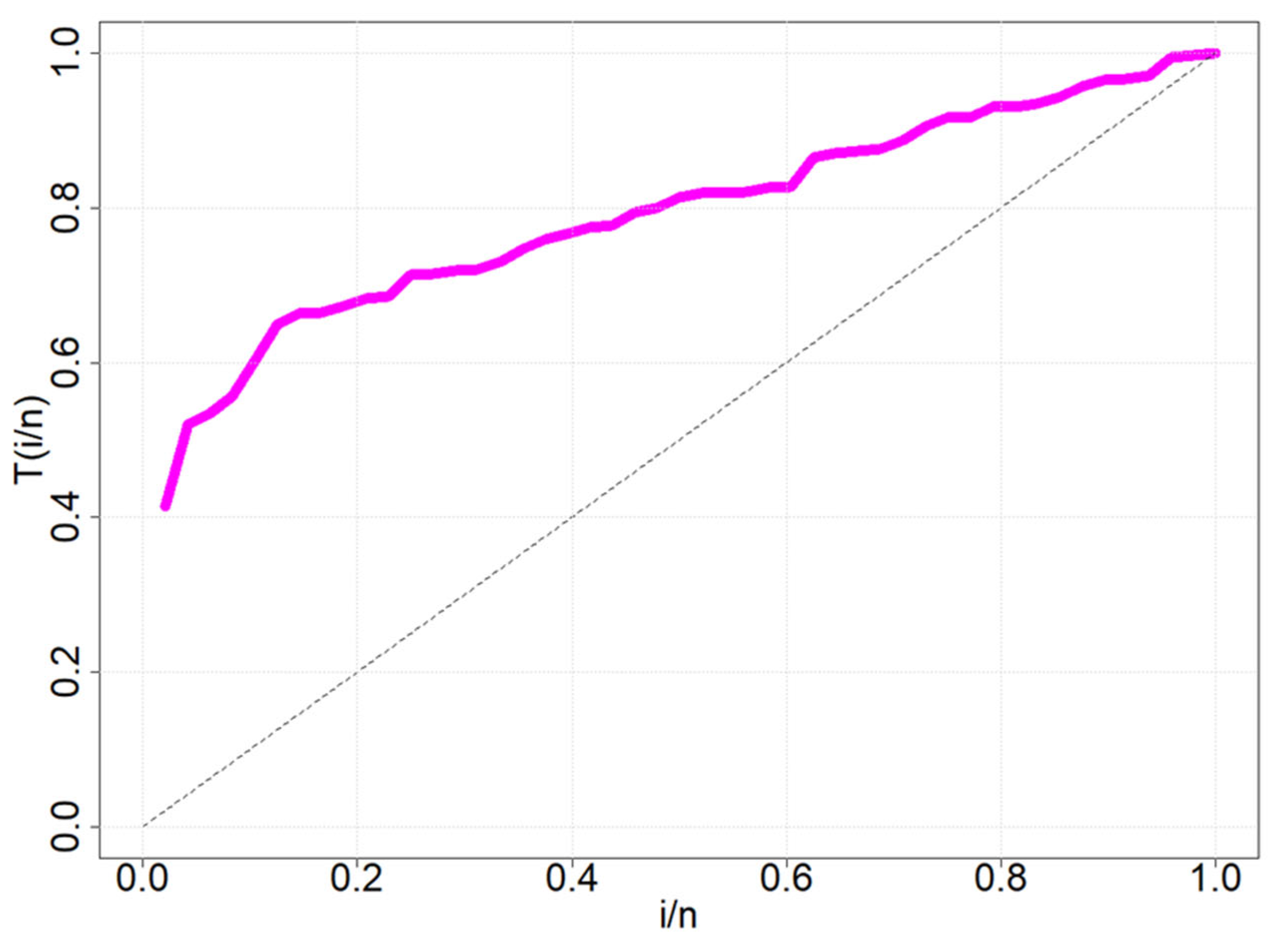
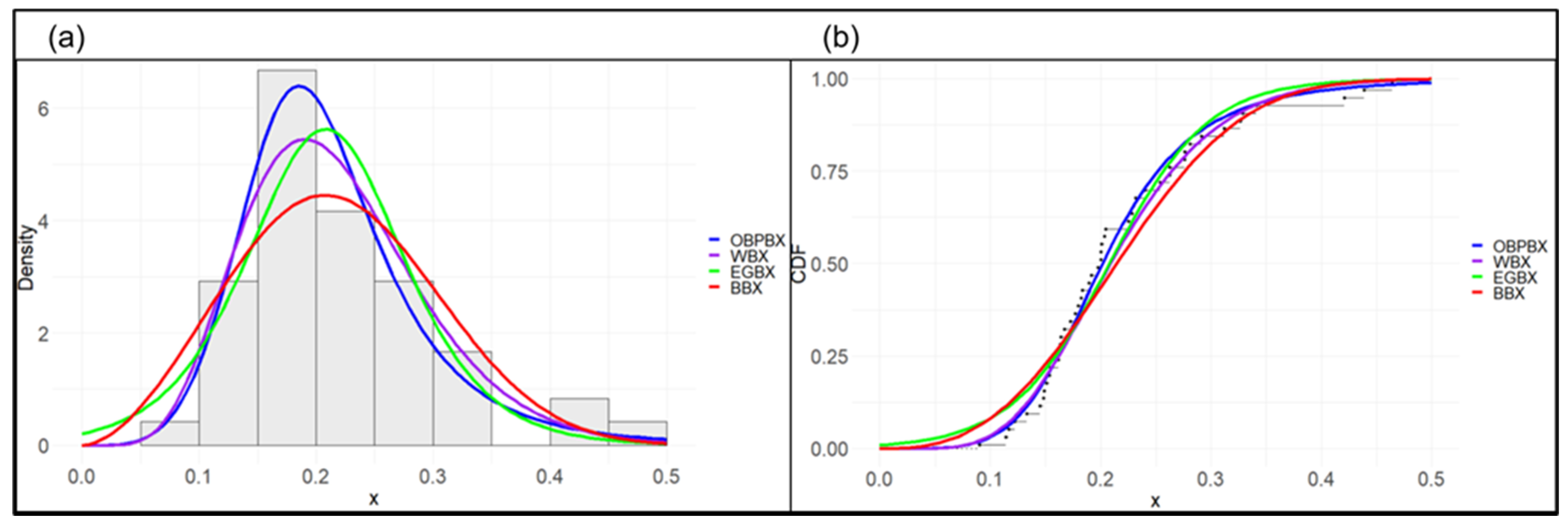
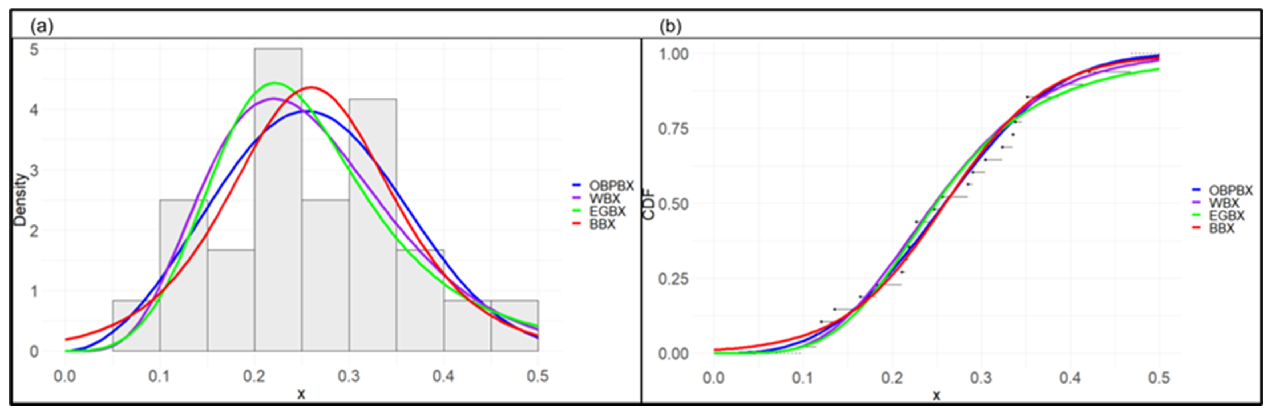
7.1. First Data Set: Petroleum Rock Sample Data
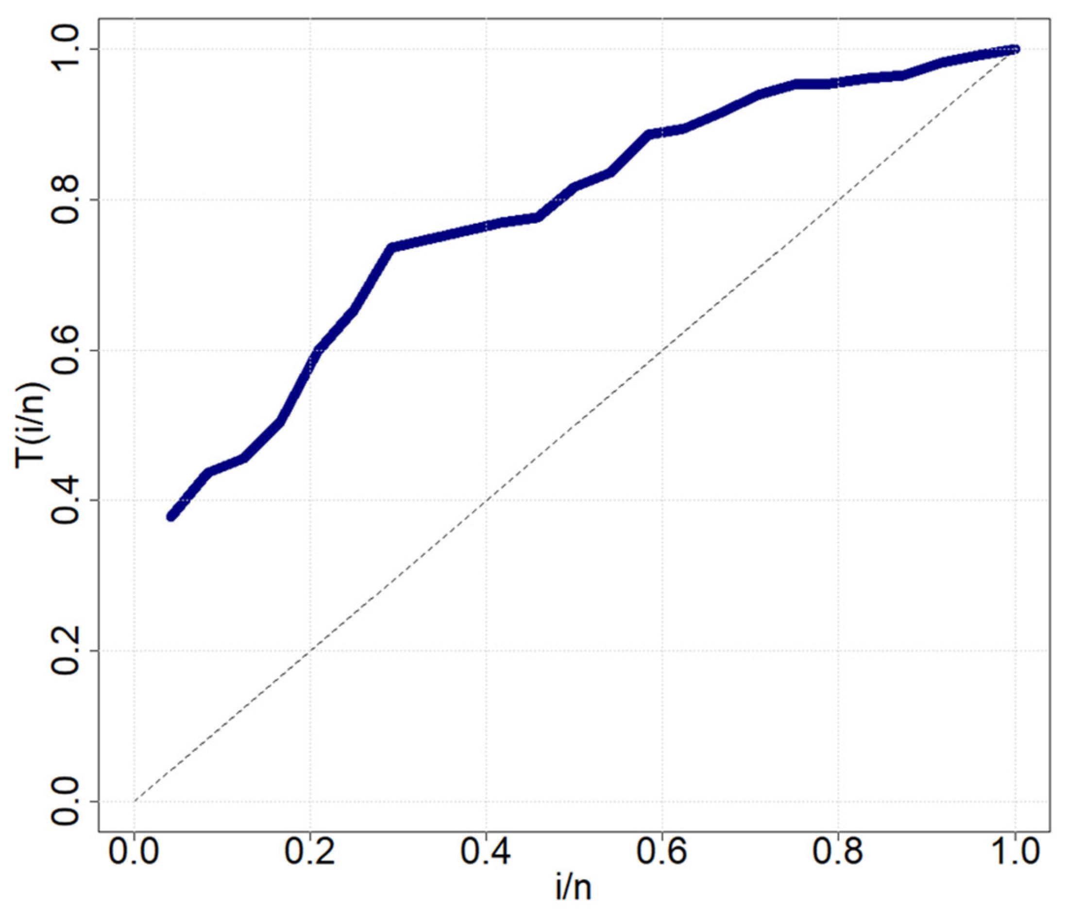
7.2. Second Data Set: United Kingdom COVID-19 Mortality Rate
8. Concluding Remarks
Author Contributions
Funding
Institutional Review Board Statement
Informed Consent Statement
Data Availability Statement
Acknowledgments
Conflicts of Interest
Nomenclature
| Random variable | |
| Cumulative distribution function of the Burr X distribution | |
| Probability density function of Burr X distribution | |
| Cumulative distribution function of the odd beta prime generalized class | |
| Probability density function of the odd beta prime generalized family | |
| Cumulative distribution function of the baseline distribution | |
| Probability density function of the baseline distribution | |
| Odd ratio | |
| Cumulative distribution function of the odd beta prime-Burr X distribution | |
| Probability density function of the odd beta prime-Burr X distribution | |
| Shape parameter | |
| Shape parameter | |
| Shape parameter | |
| Scale parameter | |
| Vector parameter | |
| Survival function | |
| Hazard function | |
| The rth moment | |
| Moment generating function | |
| The Rényi entropy | |
| The q-entropy | |
| Quantile function | |
| Continuous uniform variable | |
| Median | |
| sample size | |
| Vector parameter | |
| The likelihood function | |
| The logarithm of likelihood function | |
| The number of samples | |
| The digamma function | |
| Abbreviations | |
| OBP-G | Odd Beta Prime Generalized |
| OBPBX | Odd Beta Prime Burr X |
| CDF | Cumulative distribution function |
| Probability density function | |
| MGF | Moment generating function |
| QF | Quantile function |
| B | Bowley’s skewness |
| M | Moor’s kurtosis |
| MLE | Maximum likelihood estimation |
| MSE | Mean squared error |
| WBX | Weibull-Burr X |
| EGBX | Exponential generalized-Burr X |
| BBX | Beta-Burr X |
| AIC | Akaike information criterion |
| CAIC | Corrected Akaike information criterion |
| BIC | Bayesian information criterion |
| HQIC | Hannan–Quinn information criterion |
| TTT | Total time on test |
References
- Sherwani, R.A.K.; Ashraf, S.; Abbas, S.; Aslam, M. Marshall Olkin Exponentiated Dagum Distribution: Properties and Applications. J. Stat. Theory Appl. 2023, 22, 70–97. [Google Scholar] [CrossRef]
- Eldessouky, E.A.; Hassan, O.H.M.; Elgarhy, M.; Hassan, E.A.A.; Elbatal, I.; Almetwally, E.M. A New Extension of the Kumaraswamy Exponential Model with Modeling of Food Chain Data. Axioms 2023, 12, 379. [Google Scholar] [CrossRef]
- Fayomi, A.; Almetwally, E.M.; Qura, M.E. A novel bivariate Lomax-G family of distributions: Properties, inference, and applications to environmental, medical, and computer science data. AIMS Math. 2023, 8, 17539–17584. [Google Scholar] [CrossRef]
- Alghamdi, S.M.; Shrahili, M.; Hassan, A.S.; Gemeay, A.M.; Elbatal, I.; Elgarhy, M. Statistical Inference of the Half Logistic Modified Kies Exponential Model with Modeling to Engineering Data. Symmetry 2023, 15, 586. [Google Scholar] [CrossRef]
- Gomaa, R.S.; Magar, A.M.; Alsadat, N.; Almetwally, E.M.; Tolba, A.H. The Unit Alpha-Power Kum-Modified Size-Biased Lehmann Type II Distribution: Theory, Simulation, and Applications. Symmetry 2023, 15, 1283. [Google Scholar] [CrossRef]
- Eugene, N.; Lee, C.; Famoye, F. Beta-normal distribution and its applications. Commun. Stat.-Theory Methods 2002, 31, 497–512. [Google Scholar] [CrossRef]
- Cordeiro, G.M.; de Castro, M. A new family of generalized distributions. J. Stat. Comput. Simul. 2011, 81, 883–898. [Google Scholar] [CrossRef]
- Al-Babtain, A.A.; Shakhatreh, M.K.; Nassar, M.; Afify, A.Z. A new modified Kies family: Properties, estimation under complete and type-II censored samples, and engineering applications. Mathematics 2020, 8, 1345. [Google Scholar] [CrossRef]
- Afify, A.Z.; Al-Mofleh, H.; Aljohani, H.M.; Cordeiro, G.M. The Marshall–Olkin–Weibull-H family: Estimation, simulations, and applications to COVID-19 data. J. King Saud Univ.-Sci. 2022, 34, 102115. [Google Scholar] [CrossRef]
- Elbatal, I.; Ozel, G.; Cakmakyapan, S. Odd extended exponential-G family: Properties and application on earthquake data. J. Stat. Manag. Syst. 2022, 25, 1751–1765. [Google Scholar] [CrossRef]
- Rannona, K.; Oluyede, B.; Chipepa, F.; Makubate, B. The exponentiated odd exponential half logistic-G power series class of distributions with applications. J. Stat. Manag. Syst. 2022, 25, 1821–1848. [Google Scholar] [CrossRef]
- Iqbal, T.; Alfaer, N.M.; Tahir, M.H.; Aljohani, H.M.; Jamal, F.; Afify, A.Z. Properties and estimation approaches of the odd JCA family with applications. Concurr. Comput. Pract. Exp. 2023, 35, e7417. [Google Scholar] [CrossRef]
- El-Morshedy, M.; Tahir, M.H.; Hussain, M.A.; Al-Bossly, A.; Eliwa, M.S. A new flexible univariate and bivariate family of distributions for unit interval (0, 1). Symmetry 2022, 14, 1040. [Google Scholar] [CrossRef]
- Abbas, S.; Muhammad, M.; Jamal, F.; Chesneau, C.; Muhammad, I.; Bouchane, M. A New Extension of the Kumaraswamy Generated Family of Distributions with Applications to Real Data. Computation 2023, 11, 26. [Google Scholar] [CrossRef]
- Oluyede, B.; Chamunorwa, S.; Chipepa, F.; Alizadeh, M. The Topp-Leone Gompertz-G family of distributions with applications. J. Stat. Manag. Syst. 2022, 25, 1399–1423. [Google Scholar] [CrossRef]
- Alghamdi, A.S.; Abd El-Raouf, M.M. Exploring the Dynamics of COVID-19 with a Novel Family of Models. Mathematics 2023, 11, 1641. [Google Scholar] [CrossRef]
- Moakofi, T.; Oluyede, B. Type II Exponentiated Half-Logistic Gompertz-G Family of Distributions: Properties and Applications. Math. Slovaca 2023, 73, 785–810. [Google Scholar] [CrossRef]
- Bhatti, F.A.; Hamedani, G.; Korkmaz, M.Ç.; Yousof, H.M.; Ahmad, M. On the new modified Burr XII distribution: Development, properties, characterizations and applications. Pak. J. Stat. Oper. Res. 2023, 19, 327–348. [Google Scholar] [CrossRef]
- Alanzi, A.R.; Rafique, M.Q.; Tahir, M.; Jamal, F.; Hussain, M.A.; Sami, W. A novel Muth generalized family of distributions: Properties and applications to quality control. AIMS Math. 2023, 8, 6559–6580. [Google Scholar] [CrossRef]
- Alsolami, E.; Alsulami, D. Combining Two Exponentiated Families to Generate a New Family of Distributions. Symmetry 2022, 14, 1739. [Google Scholar] [CrossRef]
- Ristić, M.M.; Balakrishnan, N. The gamma-exponentiated exponential distribution. J. Stat. Comput. Simul. 2012, 82, 1191–1206. [Google Scholar] [CrossRef]
- Bourguignon, M.; Silva, R.B.; Cordeiro, G.M. The Weibull-G family of probability distributions. J. Data Sci. 2014, 12, 53–68. [Google Scholar] [CrossRef]
- Johnson, N.L.; Kotz, S.; Balakrishnan, N. Beta distributions. In Continuous Univariate Distributions, 2nd ed.; John Wiley and Sons: New York, NY, USA, 1994; pp. 221–235. [Google Scholar]
- Burr, I.W. Cumulative frequency functions. Ann. Math. Stat. 1942, 13, 215–232. [Google Scholar] [CrossRef]
- Hassan, O.H.M.; Elbatal, I.; Al-Nefaie, A.H.; Elgarhy, M. On the Kavya–Manoharan–Burr X Model: Estimations under Ranked Set Sampling and Applications. J. Risk Financ. Manag. 2023, 16, 19. [Google Scholar] [CrossRef]
- Surles, J.G.; Padgett, W.J. Some properties of a scaled Burr type X distribution. J. Stat. Plan. Inference 2005, 128, 271–280. [Google Scholar] [CrossRef]
- Ahmad Sartawi, H.; Abu-Salih, M.S. Bayesian prediction bounds for the Burr type X model. Commun. Stat.-Theory Methods 1991, 20, 2307–2330. [Google Scholar] [CrossRef]
- Jaheen, Z. Empirical Bayes estimation of the reliability and failure rate functions of the Burr type X failure model. J. Appl. Stat. Sci. 1996, 3, 281–288. [Google Scholar]
- Ahmad, K.; Fakhry, M.; Jaheen, Z. Empirical Bayes estimation of P (Y < X) and characterizations of Burr-type X model. J. Stat. Plan. Inference 1997, 64, 297–308. [Google Scholar]
- Surles, J.; Padgett, W. Inference for P (Y < X) in the Burr type X model. J. Appl. Stat. Sci. 1998, 7, 225–238. [Google Scholar]
- Ali Mousa, M. Inference and prediction for the Burr type X model based on records. Stat. J. Theor. Appl. Stat. 2001, 35, 415–425. [Google Scholar] [CrossRef]
- Yousof, H.M.; Afify, A.Z.; Hamedani, G.; Aryal, G.R. The Burr X Generator of Distributions for Lifetime Data. J. Stat. Theory Appl. 2017, 16, 288–305. [Google Scholar] [CrossRef]
- Ibrahim, N.A.; Khaleel, M.A. Generalizations of Burr Type X Distribution with Applications. ASM Sci. J. 2020, 13. [Google Scholar] [CrossRef] [PubMed]
- Khaleel, M.A.; Ibrahim, N.A.; Shitan, M.; Merovci, F. Some properties of Gamma Burr type X distribution with application. In Proceedings of the AIP Conference Proceedings, Yogyakarta, Indonesia, 25–26 January 2016; p. 020087. [Google Scholar]
- Ibrahim, N.A.; Khaleel, M.A.; Merovci, F.; Kilicman, A.; Shitan, M. Weibull Burr X Distribution Properties and Application. Pak. J. Stat. 2017, 33, 315–336. [Google Scholar]
- Jamal, F.; Tahir, M.; Alizadeh, M.; Nasir, M. On Marshall-Olkin Burr X family of distribution. Tbilisi Math. J. 2017, 10, 175–199. [Google Scholar] [CrossRef]
- Shrahili, M.; Elbatal, M.; Muhammad, M. The type I half-logistic Burr X distribution: Theory and practice. J. Nonlinear Sci. Appl 2019, 12, 262–277. [Google Scholar] [CrossRef][Green Version]
- Usman, R.M.; Ilyas, M. The power Burr Type X distribution: Properties, regression modeling and applications. Punjab Univ. J. Math. 2020, 52, 27–44. [Google Scholar]
- Khan, M.S.; King, R.; Hudson, I.L. Transmuted Burr type X distribution with covariates regression modeling to analyze reliability data. Am. J. Math. Manag. Sci. 2020, 39, 99–121. [Google Scholar] [CrossRef]
- Ahmed, M.T.; Khaleel, M.A.; Oguntunde, P.E.; Abdal-Hammed, M.K. A new version of the exponentiated Burr X distribution. J. Phys. Conf. Ser. 2021, 1818, 012116. [Google Scholar] [CrossRef]
- Oh, Y.L.; Lim, F.P.; Chen, C.Y.; Ling, W.S.; Loh, Y.F. Exponentiated Weibull Burr Type X Distribution’s Properties and Its Applications. Electron. J. Appl. Stat. Anal. 2022, 15, 553–573. [Google Scholar]
- Alyami, S.A.; Elbatal, I.; Alotaibi, N.; Almetwally, E.M.; Elgarhy, M. Modeling to Factor Productivity of the United Kingdom Food Chain: Using a New Lifetime-Generated Family of Distributions. Sustainability 2022, 14, 8942. [Google Scholar] [CrossRef]
- Madaki, U.Y.; Bakar, M.R.A.; Khaleel, M.A.; Handique, L. Kumaraswamy Burr Type X Distribution and Its Properties. ASEANA Sci. Educ. J. 2022, 2, 11–38. [Google Scholar]
- Koobubpha, K.; Panitanarak, T.; Domthong, P.; Panitanarak, U. The Maxwell-Burr X Distribution: Its Properties and Applications to the COVID-19 Mortality Rate in Thailand. Thail. Stat. 2023, 21, 421–434. [Google Scholar]
- Suleiman, A.; Othman, M.; Ishaq, A.; Daud, H.; Indawati, R.; Abdullah, M.L.; Husin, A. The Odd Beta Prime-G Family of Probability Distributions: Properties and Applications. Comput. Sci. Math. Forum 2023, 7, 20. [Google Scholar] [CrossRef]
- Alzaatreh, A.; Lee, C.; Famoye, F. A new method for generating families of continuous distributions. METRON 2013, 71, 63–79. [Google Scholar] [CrossRef]
- Suleiman, A.A.; Daud, H.; Singh, N.S.S.; Othman, M.; Ishaq, A.I.; Sokkalingam, R. A Novel Odd Beta Prime-Logistic Distribution: Desirable Mathematical Properties and Applications to Engineering and Environmental Data. Sustainability 2023, 15, 10239. [Google Scholar] [CrossRef]
- Ishaq, A.I.; Abiodun, A.A. The Maxwell–Weibull distribution in modeling lifetime datasets. Ann. Data Sci. 2020, 7, 639–662. [Google Scholar] [CrossRef]
- Abdullahi, U.A.; Suleiman, A.A.; Ishaq, A.I.; Usman, A.; Suleiman, A. The Maxwell–Exponential Distribution: Theory and Application to Lifetime Data. J. Stat. Model. Anal. 2021, 3, 65–80. [Google Scholar] [CrossRef]
- Klakattawi, H.S.; Aljuhani, W.H. A New Technique for Generating Distributions Based on a Combination of Two Techniques: Alpha Power Transformation and Exponentiated T-X Distributions Family. Symmetry 2021, 13, 412. [Google Scholar] [CrossRef]
- Bilal, M.; Mohsin, M.; Aslam, M. Weibull-Exponential Distribution and Its Application in Monitoring Industrial Process. Math. Probl. Eng. 2021, 2021, 6650237. [Google Scholar] [CrossRef]
- Amadu, Y.; Luguterah, A.; Nasiru, S. On the odd inverse exponential class of distributions: Properties, applications and cure fraction regression. J. Stat. Manag. Syst. 2022, 25, 805–836. [Google Scholar] [CrossRef]
- Elbatal, I.; Alotaibi, N.; Almetwally, E.M.; Alyami, S.A.; Elgarhy, M. On odd perks-G class of distributions: Properties, regression model, discretization, Bayesian and non-Bayesian estimation, and applications. Symmetry 2022, 14, 883. [Google Scholar] [CrossRef]
- Anzagra, L.; Sarpong, S.; Nasiru, S. Odd Chen-G Family of Distributions. Ann. Data Sci. 2022, 9, 369–391. [Google Scholar] [CrossRef]
- Ishaq, A.I.; Usman, A.; Tasi’u, M.; Suleiman, A.A.; Ahmad, A.G. A New Odd F-Weibull Distribution: Properties and Application of the Monthly Nigerian Naira to British Pound Exchange Rate Data. In Proceedings of the 2022 International Conference on Data Analytics for Business and Industry (ICDABI), Sakhir, Bahrain, 25–26 October 2022; pp. 326–332. [Google Scholar]
- Almetwally, E.M. The odd Weibull inverse topp–leone distribution with applications to COVID-19 data. Ann. Data Sci. 2022, 9, 121–140. [Google Scholar] [CrossRef]
- Suleiman, A.A.; Othman, M.; Ishaq, A.I.; Abdullah, M.L.; Indawati, R.; Daud, H.; Sokkalingam, R. A New Statistical Model Based on the Novel Generalized Odd Beta Prime Family of Continuous Probability Distributions with Applications to Cancer Disease Data Sets. Preprints 2022, 2022120072. [Google Scholar] [CrossRef]
- Shah, Z.; Khan, D.M.; Khan, Z.; Faiz, N.; Hussain, S.; Anwar, A.; Ahmad, T.; Kim, K.-I. A New Generalized Logarithmic—X Family of Distributions with Biomedical Data Analysis. Appl. Sci. 2023, 13, 3668. [Google Scholar] [CrossRef]
- Koleoso, P.O. The Properties of Odd Lomax-Dagum Distribution and Its Application. Sci. Afr. 2023, 19, e01555. [Google Scholar] [CrossRef]
- Suleiman, A.A.; Daud, H.; Othman, M.; Singh, N.S.S.; Ishaq, A.I.; Sokkalingam, R.; Husin, A. A Novel Extension of the Fréchet Distribution: Statistical Properties and Application to Groundwater Pollutant Concentrations. J. Data Sci. Insights 2023, 1, 8–24. [Google Scholar]
- Khadim, A.; Saghir, A.; Hussain, T.; Shakil, M. Some new developments and review on TX family of distributions. J. Stat. Appl. Pro 2022, 11, 739–757. [Google Scholar]
- Suleiman, A.A.; Suleiman, A.; Abdullahi, U.A.; Suleiman, A.S. Estimation of the case fatality rate of COVID-19 epidemiological data in Nigeria using statistical regression analysis. Biosafety and Health 2021, 3, 4–7. [Google Scholar] [CrossRef]
- Fayomi, A.; Hassan, A.S.; Baaqeel, H.; Almetwally, E.M. Bayesian Inference and Data Analysis of the Unit–Power Burr X Distribution. Axioms 2023, 12, 297. [Google Scholar] [CrossRef]
- Oh, Y.L.; Lim, F.P.; Chen, C.Y.; Ling, W.S.; Loh, Y.F. A New Exponentiated Beta Burr Type X Distribution: Model, Theory, and Applications. Sains Malays. 2023, 52, 281–294. [Google Scholar] [CrossRef]
- Elbatal, I.; Alghamdi, S.M.; Ghorbal, A.B.; Shawki, A.; Elgarhy, M.; El-Saeed, A.R. Exponentiated Kavya-Manoharan Burr X Distribution: Estimation under Censored Type Ii with Applications in Medical Data. JP J. Biostat. 2023, 23, 227–247. [Google Scholar] [CrossRef]
- Tlhaloganyang, B.P.; Sengweni, W.; Oluyede, B. The The Gamma Odd Burr XG Family of Distributions with Applications. Pak. J. Stat. Oper. Res. 2022, 18, 721–746. [Google Scholar] [CrossRef]
- Alshanbari, H.M.; Odhah, O.H.; Almetwally, E.M.; Hussam, E.; Kilai, M.; El-Bagoury, A.-A.H. Novel Type I Half Logistic Burr-Weibull Distribution: Application to COVID-19 Data. Comput. Math. Methods Med. 2022, 2022, 1444859. [Google Scholar] [CrossRef] [PubMed]
- Al Sobhi, M.M. Statistical Inference and Mathematical Properties of Burr X Logistic-Exponential Distribution with Applications to Engineering Data. J. Math. 2022, 2022, 4688871. [Google Scholar] [CrossRef]
- Ade, O.A.; Osezuwa, O.I.; Adeniji, O.E.; Adelekan, O.G. Generalized Bur X Lomax Distribution: Properties, Inference and Application to Aircraft Data. J. Math. Res. 2022, 14, 1–52. [Google Scholar]
- Al-Babtain, A.A.; Elbatal, I.; Al-Mofleh, H.; Gemeay, A.M.; Afify, A.Z.; Sarg, A.M. The Flexible Burr X-G Family: Properties, Inference, and Applications in Engineering Science. Symmetry 2021, 13, 474. [Google Scholar] [CrossRef]
- Bantan, R.A.R.; Chesneau, C.; Jamal, F.; Elbatal, I.; Elgarhy, M. The Truncated Burr X-G Family of Distributions: Properties and Applications to Actuarial and Financial Data. Entropy 2021, 23, 1088. [Google Scholar] [CrossRef]
- Karamikabir, H.; Afshari, M.; Alizadeh, M.; Yousof, H.M. The odd log-logistic burr-x family of distributions: Properties and applications. J. Stat. Theory Appl. 2021, 20, 228–241. [Google Scholar] [CrossRef]
- Algarni, A.; M. Almarashi, A.; Elbatal, I.; S. Hassan, A.; Almetwally, E.M.; M. Daghistani, A.; Elgarhy, M. Type I Half Logistic Burr X-G Family: Properties, Bayesian, and Non-Bayesian Estimation under Censored Samples and Applications to COVID-19 Data. Math. Probl. Eng. 2021, 2021, 5461130. [Google Scholar] [CrossRef]
- Abdelkhalek, R.H. The Poisson Burr X Inverse Rayleigh Distribution And Its Applications. J. Data Sci. 2020, 18, 56–77. [Google Scholar] [CrossRef]
- Butt, N.S.; Khalil, M.G. A New Bimodal Distribution for Modeling Asymmetric Bimodal Heavy-Tail Real Lifetime Data. Symmetry 2020, 12, 2058. [Google Scholar] [CrossRef]
- Usman, R.M.; Handique, L.; Chakraborty, S. Some Aspects of the Odd Log-Logistic Burr X Distribution with Applications in Reliability Data Modeling. Int. J. Appl. Math. Stat. 2019, 58, 127–147. [Google Scholar]
- Yousof, H.; Jahanshahi, S.; Sharma, V.K. The Burr X Fréchet model for extreme values: Mathematical properties, classical inference and Bayesian analysis. Pak. J. Stat. Oper. Res. 2019, 15, 797–818. [Google Scholar] [CrossRef]
- Abouelmagd, T.; Hamed, M.S.; Hamedani, G.; Ali, M.; Goual, H.; Korkmaz, M.; Yousof, H.M. The zero truncated Poisson Burr X family of distributions with properties, characterizations, applications, and validation test. J. Nonlinear Sci. Appl. 2019, 12, 314–336. [Google Scholar] [CrossRef]
- Abouelmagd, T.; Hamed, M.S.; Yousof, H.M. Poisson Burr X Weibull distribution. J. Nonlinear Sci. Appl. 2019, 12, 173–183. [Google Scholar] [CrossRef]
- Aldahlan, M.A. A new three-parameter lifetime distribution: Properties and applications. Int. J. Innov. Sci. Math. 2019, 7, 54–66. [Google Scholar]
- Khalil, M.G.; Hamedani, G.G.; Yousof, H.M. The Burr X exponentiated Weibull model: Characterizations, mathematical properties and applications to failure and survival times data. Pak. J. Stat. Oper. Res. 2019, 15, 141–160. [Google Scholar] [CrossRef]
- Elsayed, H.; Yousof, H. The Burr X Nadarajah Haghighi distribution: Statistical properties and application to the exceedances of flood peaks data. J. Math. Stat. 2019, 15, 146–157. [Google Scholar] [CrossRef]
- Abdullah, Z.M.; Khaleel, M.A.; Abdal-hameed, M.K.; Oguntunde, P.E. Estimating Parameters for Extension of Burr Type X Distribution by Using Conjugate Gradient in Unconstrained Optimization. Kirkuk Univ. J. Sci. Stud. 2019, 14, 33–49. [Google Scholar] [CrossRef]
- Khaleel, M.A.; Ibrahim, N.A.; Shitan, M.; Merovci, F. New extension of Burr type X distribution properties with application. J. King Saud Univ.-Sci. [CrossRef]
- Refaie, M.K. Burr X exponentiated exponential distribution. J. Stat. Appl. 2018, 1, 71–88. [Google Scholar]
- Jamal, F.; Nasir, M.A. Generalized Burr X family of distributions. Int. J. Math. Stat. 2018, 19, 1–20. [Google Scholar]
- Madaki, U.Y.; Abu Bakar, M.R.; Handique, L. Beta Kumaraswamy Burr Type X Distribution and Its Properties. Preprints 2018, 2018080356. [Google Scholar] [CrossRef]
- Ishaq, A.; Usman, A.; Tasi’u, M.; Aliyu, Y. Weibull-Burr type x distribution: Its properties and application. Niger. J. Sci. Res. 2017, 16, 150–157. [Google Scholar]
- Korkmaz, M.Ç.; Altun, E.; Yousof, H.M.; Afify, A.Z.; Nadarajah, S. The Burr X Pareto Distribution: Properties, Applications and VaR Estimation. J. Risk Financ. Manag. 2018, 11, 1. [Google Scholar] [CrossRef]
- Zayed, M.; Butt, N.S. The extended Fréchet distribution: Properties and applications. Pak. J. Stat. Oper. Res. 2017, 13, 529–543. [Google Scholar] [CrossRef][Green Version]
- Al-Saiari, A.Y.; Baharith, L.A.; Mousa, S.A. New extended burr type X distribution. Sri Lankan J. Appl. Stat. 2016, 17, 217–231. [Google Scholar] [CrossRef]
- Merovci, F.; Khaleel, M.A.; Ibrahim, N.A.; Shitan, M. The beta Burr type X distribution properties with application. SpringerPlus 2016, 5, 697. [Google Scholar] [CrossRef]
- Zwillinger, D.; Jeffrey, A. Table of Integrals, Series, and Products; Elsevier: Burlington, USA, 2007. [Google Scholar]
- Kenney, J.F.; Keeping, E.S. Mayhematics of Statistics; van Nostrand, D., Ed.; D. Van Nostrand Company: New York, NY, USA, 1939. [Google Scholar]
- Moors, J. A quantile alternative for kurtosis. J. R. Stat. Soc. Ser. D 1988, 37, 25–32. [Google Scholar] [CrossRef]
- Nasir, M.A.; Tahir, M.; Jamal, F.; Ozel, G. A new generalized Burr family of distributions for the lifetime data. J. Stat. Appl. Probab. 2017, 6, 401–417. [Google Scholar] [CrossRef]
- Singh, V.V.; Suleman, A.A.; Ibrahim, A.; Abdullahi, U.A.; Suleiman, S.A. Assessment of probability distributions of groundwater quality data in Gwale area, north-western Nigeria. Ann. Optim. Theory Pract. 2020, 3, 37–46. [Google Scholar]
- Auwalu, I.; Suleiman, A.A.; Abdullahi, U.A.; Suleiman, A.S. Monitoring Groundwater Quality using Probability Distribution in Gwale, Kano state, Nigeria. J. Stat. Model. Anal. 2021, 3, 95–108. Available online: http://jummec.um.edu.my/index.php/JOSMA/article/view/32362 (accessed on 25 July 2023).
- Moutinho Cordeiro, G.; dos Santos Brito, R. The beta power distribution. Braz. J. Probab. Stat. 2012, 26, 88–112. [Google Scholar] [CrossRef]


| Parameter | n | Mean | Bias | MSE | Mean | Bias | MSE |
|---|---|---|---|---|---|---|---|
| 15 | 0.541404 | 0.025403 | 0.002630 | 1.545356 | 0.005950 | 0.008764 | |
| 25 | 0.540392 | 0.025215 | 0.002429 | 1.524563 | 0.005755 | 0.008384 | |
| 50 | 0.537420 | 0.021420 | 0.002134 | 1.515567 | 0.005452 | 0.007845 | |
| 75 | 0.532419 | 0.021053 | 0.002035 | 1.509634 | 0.005358 | 0.005647 | |
| 100 | 0.531406 | 0.011402 | 0.000130 | 1.506465 | 0.004251 | 0.002637 | |
| 150 | 0.528139 | 0.011213 | 0.000126 | 1.502745 | 0.003351 | 0.000864 | |
| 200 | 0.523918 | 0.011191 | 0.000122 | 1.501351 | 0.002935 | 0.000176 | |
| 15 | 1.067935 | −0.00108 | 0.004533 | 0.042320 | −0.15761 | 0.024862 | |
| 25 | 1.068648 | −0.00117 | 0.002436 | 0.042314 | −0.15768 | 0.022435 | |
| 50 | 1.068823 | −0.00119 | 0.001624 | 0.042260 | −0.15779 | 0.021534 | |
| 75 | 1.068931 | −0.00122 | 0.000764 | 0.075674 | −0.15946 | 0.020455 | |
| 100 | 1.069034 | −0.00126 | 0.000663 | 0.093452 | −0.16374 | 0.019674 | |
| 150 | 1.069532 | −0.00132 | 0.000534 | 0.142654 | −0.16747 | 0.014868 | |
| 200 | 1.069720 | −0.00139 | 0.000243 | 0.195432 | −0.20125 | 0.011367 | |
| 15 | 1.255833 | 0.005832 | 0.093542 | 0.755199 | 0.005199 | 0.009354 | |
| 25 | 1.254828 | 0.004828 | 0.054232 | 0.755200 | 0.005201 | 0.008464 | |
| 50 | 1.254245 | 0.004739 | 0.023547 | 0.755197 | 0.005197 | 0.005631 | |
| 75 | 1.253837 | 0.004236 | 0.008452 | 0.755201 | 0.005205 | 0.003569 | |
| 100 | 1.253132 | 0.004132 | 0.005432 | 0.755201 | 0.005201 | 0.002345 | |
| 150 | 1.252833 | 0.003830 | 0.003745 | 0.755204 | 0.005197 | 0.000935 | |
| 200 | 1.250829 | 0.002828 | 0.009543 | 0.755205 | 0.005141 | 0.000438 | |
| 15 | 0.225331 | 0.687564 | 0.885534 | 1.348640 | 0.019592 | 0.019354 | |
| 25 | 0.225196 | 0.683885 | 0.821651 | 1.404465 | 0.015593 | 0.017457 | |
| 50 | 0.201484 | 0.655484 | 0.765274 | 1.426411 | 0.013588 | 0.013219 | |
| 75 | 0.182574 | 0.605392 | 0.652271 | 1.436756 | 0.008592 | 0.006351 | |
| 100 | 0.129271 | 0.555271 | 0.615527 | 1.446405 | 0.006594 | 0.003238 | |
| 150 | 0.102522 | 0.465486 | 0.565141 | 1.468564 | 0.005597 | 0.000948 | |
| 200 | 0.092255 | 0.495570 | 0.486535 | 1.494783 | 0.003599 | 0.000374 | |
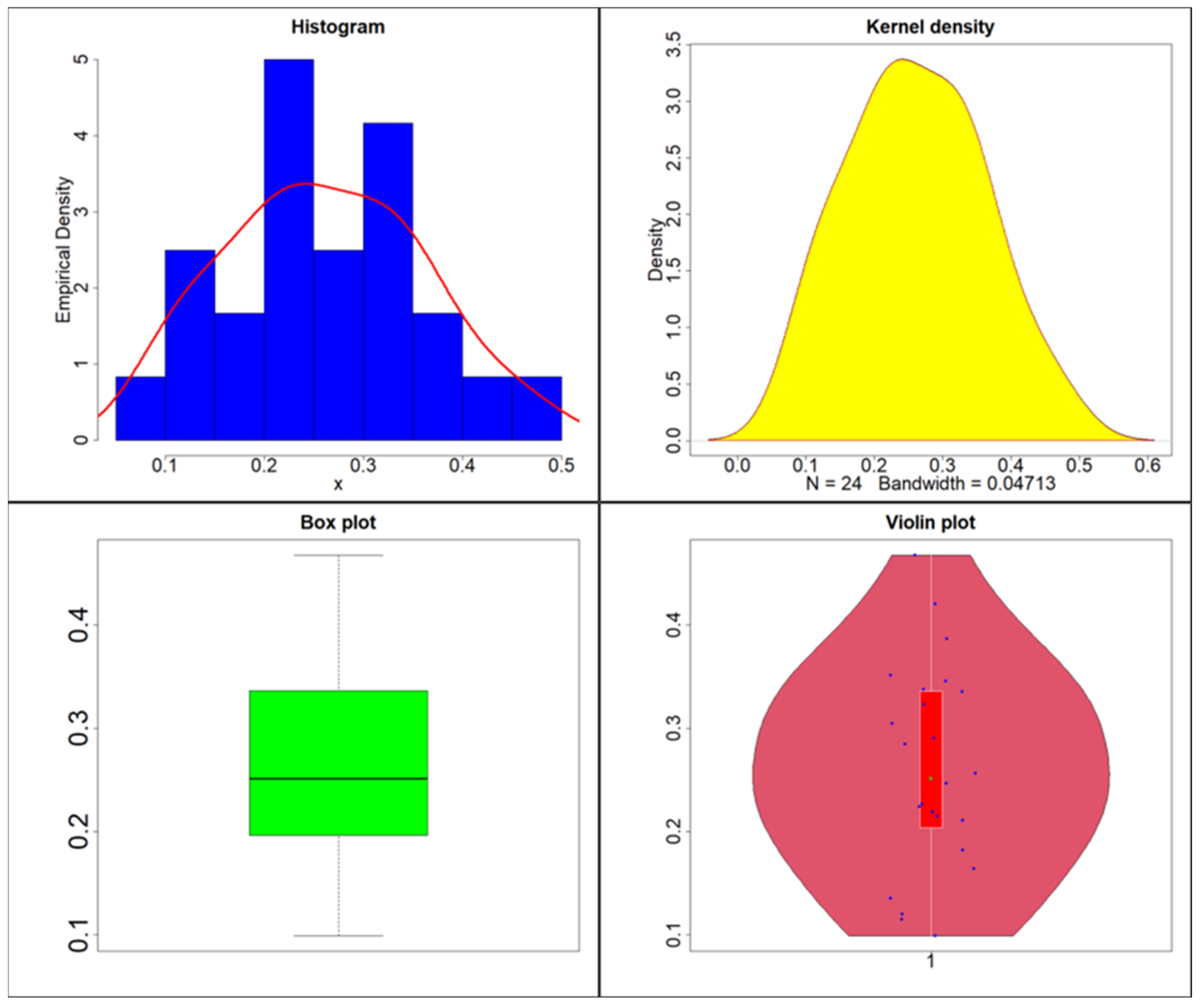
| Data | Min | Q1 | Q3 | Median | Mean | Max | Variance | Skewness | Kurtosis |
|---|---|---|---|---|---|---|---|---|---|
| Petroleum | 0.090 | 0.162 | 0.263 | 0.199 | 0.218 | 0.464 | 0.007 | 1.133 | 0.940 |
| Model | Estimates | Fitted Measures | |||||||
|---|---|---|---|---|---|---|---|---|---|
| AIC | CAIC | BIC | HQIC | ||||||
| OBPBX | 0.3744 (0.0536) | 1.0933 (0.3242) | 1.4102 (0.5343) | 1.9231 (0.6301) | 25.659 | −43.318 | −42.388 | −35.833 | −40.490 |
| WBX | 0.2535 (0.0342) | 0.9017 (0.1425) | 0.8647 (0.4326) | 0.9985 (0.5362) | 16.072 | −24.143 | −23.213 | −16.658 | −21.315 |
| EGBX | 0.6911 (0.3242) | 1.0313 (0.0746) | 0.9975 (0.8625) | 0.4525 (0.0240) | 5.063 | −2.126 | −1.196 | 5.359 | 0.702 |
| BBX | 0.5662 (0.2614) | 1.0680 (0.5342) | 0.6806 (0.4231) | 0.9948 (0.2015) | −5.191 | −2.383 | −1.452 | 5.102 | 0.446 |
| Data | Min | Q1 | Q3 | Median | Mean | Max | Variance | Skewness | Kurtosis |
|---|---|---|---|---|---|---|---|---|---|
| COVID-19 | 0.099 | 0.203 | 0.336 | 0.252 | 0.261 | 0.4678 | 0.010 | 0.152 | −0.902 |
| Model | Estimates | Fitted Measures | |||||||
|---|---|---|---|---|---|---|---|---|---|
| AIC | CAIC | BIC | HQIC | ||||||
| OBPBX | 0.5662 (0.2853) | 1.0680 (0.0546) | 1.3613 (0.7034) | 1.9897 (1.0745) | 11.549 | −15.097 | −12.992 | −10.385 | −13.847 |
| WBX | 0.1550 (0.0234) | 0.9267 (0.5362) | 0.7583 (0.1901) | 0.9495 (0.5462) | 2.114 | 3.772 | 5.878 | 8.485 | 5.022 |
| EGBX | 0.7293 (0.2324) | 1.0833 (0.3425) | 0.9026 (0.4319) | 0.4920 (0.0183) | 0.670 | 6.661 | 8.766 | 11.373 | 7.911 |
| BBX | 0.5662 (0.2340) | 1.0680 (0.5362) | 0.6806 (0.3425) | 0.9948 (0.3211) | 1.257 | 5.486 | 7.592 | 10.199 | 6.736 |
Disclaimer/Publisher’s Note: The statements, opinions and data contained in all publications are solely those of the individual author(s) and contributor(s) and not of MDPI and/or the editor(s). MDPI and/or the editor(s) disclaim responsibility for any injury to people or property resulting from any ideas, methods, instructions or products referred to in the content. |
© 2023 by the authors. Licensee MDPI, Basel, Switzerland. This article is an open access article distributed under the terms and conditions of the Creative Commons Attribution (CC BY) license (https://creativecommons.org/licenses/by/4.0/).
Share and Cite
Suleiman, A.A.; Daud, H.; Singh, N.S.S.; Ishaq, A.I.; Othman, M. A New Odd Beta Prime-Burr X Distribution with Applications to Petroleum Rock Sample Data and COVID-19 Mortality Rate. Data 2023, 8, 143. https://doi.org/10.3390/data8090143
Suleiman AA, Daud H, Singh NSS, Ishaq AI, Othman M. A New Odd Beta Prime-Burr X Distribution with Applications to Petroleum Rock Sample Data and COVID-19 Mortality Rate. Data. 2023; 8(9):143. https://doi.org/10.3390/data8090143
Chicago/Turabian StyleSuleiman, Ahmad Abubakar, Hanita Daud, Narinderjit Singh Sawaran Singh, Aliyu Ismail Ishaq, and Mahmod Othman. 2023. "A New Odd Beta Prime-Burr X Distribution with Applications to Petroleum Rock Sample Data and COVID-19 Mortality Rate" Data 8, no. 9: 143. https://doi.org/10.3390/data8090143
APA StyleSuleiman, A. A., Daud, H., Singh, N. S. S., Ishaq, A. I., & Othman, M. (2023). A New Odd Beta Prime-Burr X Distribution with Applications to Petroleum Rock Sample Data and COVID-19 Mortality Rate. Data, 8(9), 143. https://doi.org/10.3390/data8090143