A Mixture Hidden Markov Model to Mine Students’ University Curricula

Abstract

In the context of higher education, the wide availability of data gathered by universities for administrative purposes or for recording the evolution of students’ learning processes makes novel data mining techniques particularly useful to tackle critical issues. In Italy, current academic regulations allow students to customize the chronological sequence of courses they have to attend to obtain the final degree. This leads to a variety of sequences of exams, with an average time taken to obtain the degree that may significantly differ from the time established by law. In this contribution, we propose a mixture hidden Markov model to classify students into groups that are homogenous in terms of university paths, with the aim of detecting bottlenecks in the academic career and improving students’ performance.

1. Introduction

In the context of higher education, the wide availability of administrative data has significantly grown in the last decade, making learning analytics techniques particularly useful to face critical issues, and providing insights that can benefit students, teacher staff, and policy makers. In this setting, educational data mining is a discipline that has recently emerged in the broader research area of data mining, with the aim of developing methods for the analysis of all information arising in the educational context [1], that is, information gathered both for administrative purposes and for recording the evolution of learning processes, or data coming from innovative learning evaluation techniques (for details see http://www.educationaldatamining.org/, accessed date: 18 January 2022). By combining tools and solutions belonging to the scientific areas of computer science, education, and statistics, educational data mining techniques allow us to understand students’ behaviour, to facilitate the growth of their knowledge and to improve their skills, but also to design better and smarter ways of teaching. For a review of the possible applications and the huge amount of works published in such settings, see, among others, [2,3,4,5], and references therein.

In Italy, academic regulations provide that the final degree is awarded after a series of courses, at the end of which it is compulsory to take the related exam. The courses that characterise the plan of study of a degree program are divided into basic courses properly linked to the educational objectives (in terms of skills and knowledge) of the bachelor’s or master’s degree, additional courses that must be chosen from a broader set that still characterises the course of study, and a residual small part of free choice courses. Each student presents a plan of exams distributed along a certain time period established by law (three years for bachelor’s degree programs and two years for master’s degree programs). However, academic regulations also allow students to customise the chronological sequence of attended courses and to postpone the related exams with respect to the plan. This leads to many different sequences of taken exams with related different times to complete the study plan, which can often go beyond the lawful term (i.e., three or two years). In such a context, identifying career paths that are particularly virtuous in terms of degree grade and time to qualification, as well as courses representing “bottlenecks” in the students’ careers, is especially relevant for the university management in order to plan and optimise the degree programs and improve the academic guidance services.

The literature presents various papers on this particular topic. Campagni et al. [6] analysed academic student careers using a geometrical approach that combines sequential pattern analysis and cluster analysis. Their approach makes it possible to compare the observed student careers with an ideal and to correlate them with exam performance, so as to assess if a degree program is well structured. Bacci et al. [7] analysed the performance of academic students in the first year through a semi-parametric item response theory model that jointly accounts for the observed exam performances and for the information on the postponed exams; individual characteristics are also included in the model. Their work focuses on first-year exams and does not explicitly account for the chronological sequence of enrolled exams. Campagni et al. [8] applied a cluster analysis to assess how the performance during the first year affects academic career during the following years. Berens et al. [9] proposed an algorithm that combines logit regression modelling, neural networks modelling, and decision trees to predict the potential dropout of academic pupils, using institutional administrative data gathered on their careers. Pelaez et al. [10] follow a model-based approach: they implement a hierarchical clustering on latent class trees to identify at-risk students that could benefit from supplemental instruction programs. Wong and Yip [11] compare various decision tree algorithms to classify students according to abilities, diligence, motivation, and activity in order to predict their performance.

In this contribution, we propose a methodological approach to study the entire chronological sequence of exams taken by students, with the aim of identifying homogenous groups (latent classes) of students and detecting problematic exams for each latent class; individual covariates are also accounted for in the clustering process. With respect to the above cited works, our proposal takes into account all the exams of the degree program and the observed chronological sequence of taken exams; moreover, with respect to the works [6,8,11] we adopt a model-based approach.

The study is based on a cohort of students enrolled in the bachelor’s degree program in Business Economics of the University of Florence (Italy) in the year 2012 and followed up to the year 2018. The data at issue present the typical structure of multichannel or multidimensional sequence data, where the term “sequence” refers to each single course planned in the degree program and consists of an ordered set of binary states (i.e., exam taken or not yet taken) that are observed in certain time occasions. Time occasions correspond to the exam sessions (eight exam sessions by year) and the observed state at a given time reflects if the related exam has been taken at that occasion or before. Sequences have an individual-specific length, depending on the time a student takes to conclude the degree program. It is worth observing that in the Italian academic archives failed exams may not be registered; thus, the distinction between not taken and taken but failed exams is not available. In what follows, the expression “taken” implies “taken and passed” exam, whereas “not taken” stands for “not taken or taken but failed” exam.

The literature about the analysis of sequence data distinguishes two main approaches, both of them aimed at studying how sequences of categorical (e.g., binary) states change along time: the optimal matching approach and the latent variable modelling approach. Optimal matching (for an exhaustive review see [12]; see also [13] for a recent generalisation for multichannel sequence data), usually associated with cluster analysis, is a model-free data-driven approach based on dissimilarity measures between sequences. The main aim of optimal matching consists of finding typical and atypical patterns in state sequences. Optimal matching represents a satisfactory approach to describe and explore the (usually complex) structure of sequence data; however, it does not allow inferences to be made.

As opposed to the optimal matching, model-based approaches embed the analysis of sequence data in a probabilistic framework with benefits in terms of the generalisability of results. In such a context, latent variable models for longitudinal data represent a wide class of models [14,15], which provides several alternatives to properly take into account the main characteristics of sequence data, that is, (i) serial dependence or autocorrelation (i.e., the correlation between the responses of the same individual), (ii) unobserved heterogeneity in the individuals (i.e., variability in the data that is due to unobservable individual characteristics), and (iii) the dependence of the observed data on covariates.

Latent variable models account for unobserved heterogeneity by means of random effects at the individual level. Random effects can have a continuous or a discrete distribution and can be time-constant or time-varying. The discreteness assumption presents several advantages with respect to continuity. First, it avoids unnecessary distributional assumptions and it substantially reduces the computational effort, which is commonly encountered to maximise the log-likelihood function in the presence of complex data structures. Moreover, treating unobserved heterogeneity as a continuous random effect is not satisfactory when clustering individuals in homogenous groups is of interest in the study, as in the present contribution. Models assuming the discreteness of latent variables are also known as latent variable mixture models [16,17].

In the class of latent variable mixture models, we consider the mixture growth models [18,19,20] and the Hidden Markov (HM; or latent Markov) models [21,22]. Mixture growth models adopt time-constant random effects (i.e., random intercept and random slopes) that identify the time trajectories shared by individuals belonging the same group. In contrast, in the HM models a finite, and usually small, number of time-varying random effects is introduced to explain the generation process of the sequence of observed states. These random effects, usually known as hidden or latent states, are assumed to follow a first-order Markov chain. Individuals are allowed to move from a hidden state to another along the time and those that belong to the same hidden state at a certain time point have the same probability of manifesting a certain observed state. For the aim of this contribution, HM models are more suitable than mixture growth models, as they take into account the realistic possibility that an individual changes their own state, as their academic career gradually advances. For other works that adopt HM-based approaches in the educational setting, see, among others, [23,24,25].

An interesting generalization of the basic HM model is represented by the Mixture HM (MHM) model [26,27,28,29], which characterizes the concomitant presence of both time-varying (as in the basic HM model) and time-constant (as in the basic latent class model; [30,31]) discrete random effects. Time-varying effects deal with the unobserved heterogeneity that changes over time, whereas time-constant effects take into account the presence of unobservable groups, or latent classes, of individuals in the population sharing time-constant homogenous characteristics, with each of these groups following a specific HM model. Membership to latent classes may be assumed to depend on individual covariates, as in the concomitant variables approach [32,33].

In this contribution, the approach we adopt is based on the formulation and estimation of an MHM model with concomitant variables. In detail, the model we propose is composed of three parts: (i) an HM sub-model to account for the serial dependence as well as the time-varying unobserved heterogeneity, (ii) a latent class sub-model to deal with the time-constant unobserved heterogeneity, and (iii) a multinomial logit sub-model to deal with the dependence of latent class membership on individual characteristics.

The remainder of the paper is organised as follows. In Section 2, the structure of data is described, whereas a detailed description of the adopted methodological approach is illustrated in Section 3. In Section 4, we provide details about the model specification and we also describe and discuss results related to the model estimation. Finally, Section 5 reports the main conclusions.

2. Data Description

The analysis proposed here is based on a cohort of 290 students enrolled in the bachelor’s degree program in Business Economics of the University of Florence (Italy) in the year 2012 and followed up to the year 2018. The degree course is structured along a period of three years, during which any student has to attend twenty-two courses and to take the corresponding final tests. For a preliminary descriptive analysis of this cohort of students see [34].

The analyses presented in this contribution were performed on courses that were taken by at least ten students. A total number of 28 courses were therefore included. For the sake of parsimony, only results related to the six first-year courses are shown here (complete results are available from the authors upon request), which are all compulsory and consist of: Accounting, Mathematics, and Private Law, scheduled at the end of the first semester of the first year, and Management, Microeconomics, and Statistics, scheduled at the end of the second semester of the first year. Indeed, previous studies (see, among others, Ref. [7]) confirm that the performance of freshmen in the first year of their academic life is of primary relevance to predict the final results in terms of both university final grade and time to qualification.

As outlined in the Introduction, we are here mainly focused on the chronological sequences of courses (rather than on the exam grade points), with each sequence characterised by a dichotomous observed state, denoting if the exam has been taken at a certain exam session (or before) or not; eight exam sessions are available every year.

From a theoretical point of view, exams related to courses scheduled in the first year are expected to be taken in one of the eight exam sessions of the first year (i.e., sessions 1 to 8), exams related to courses scheduled in the second year are expected to be taken in one of the eight sessions of the second year (i.e., sessions 9 to 16), and similarly, exams related to courses scheduled in the third year are expected to be taken in one of the eight sessions of the third year (i.e., sessions 17 to 24). However, as in the Italian university system students can freely decide when to take an exam, in practice we often observe that certain exams tend to be postponed, mainly when they are perceived as particularly difficult. The most evident effect of the attitude to postponing exams is that many students take exams also after the third academic year and, then, the actual duration of a three-year degree course is much longer than the three years formally scheduled in the student’s degree program. For example, 20.7% of the students enrolled in Business Economics in 2012 (60 out of 290 students) had not yet graduated at the end of the year 2018, that is, six years after enrolment.

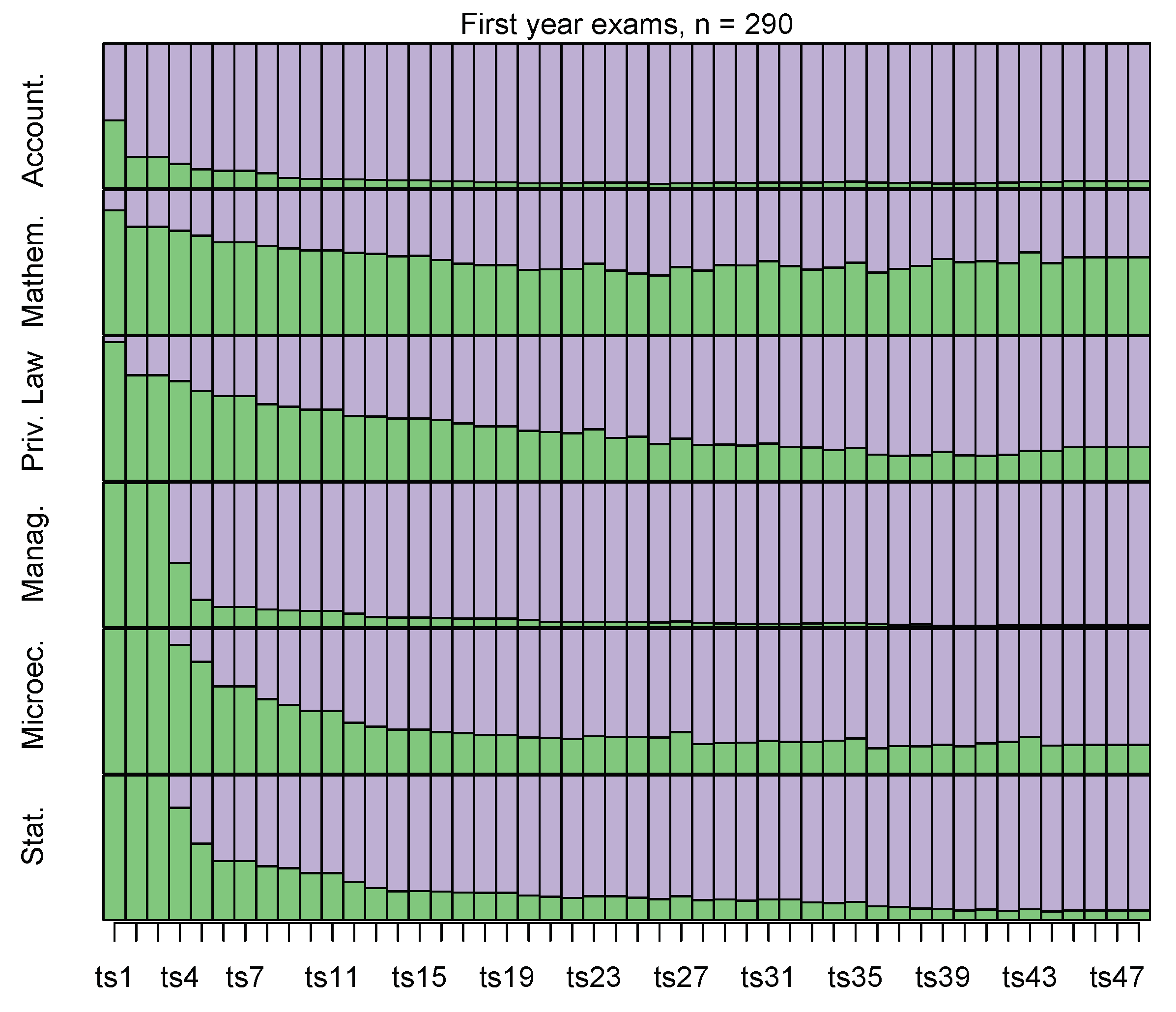
In the following, Figure 1, Figure 2 and Figure 3 show the distribution of the cohort of students along the period 2012–2018, separately for each first-year course. For each exam session ($ts1,\dots ,ts48$ on the x-axis of plots), the proportion of students that have taken the final test is depicted through a purple rectangle and the complementary proportion of students that have not yet taken the exam is depicted through a green rectangle.

As shown in Figure 1, postponing exams involves shares of students that are particularly relevant for certain courses. On one hand, Accounting and Management do not present any particular problem, as the majority of students takes the related exams within the end of the first academic year (exam sessions 1 to 8). On the other hand, Mathematics, Private Law and Microeconomics present a long tail of postponements, thus students that are still enrolled at the end of the period of follow up have not yet taken these exams.

In Figure 2, the chronological sequences of first-year courses are shown according to some baseline individual characteristics, that is, gender (males vs. females; top panel), type of high school (HS; middle panel), and HS final grade (values in the range 60–100; bottom panel).

Variable HS type distinguishes among schools that provide a strong theoretical background, such as humanistic and scientific HS (52.1% of individuals), and schools that are mainly oriented to the needs of the job context and provide practical skills, mainly in accounting; in this latter case, we separate technical HS (28.3%) and vocational HS or others (e.g., foreign language HS; 19.7%). No significant difference is observed between females and males, whereas both the HS type and the HS final grade suggest an association with the tendency to postpone exams. In detail, students coming from a vocational or other type of HS, followed by colleagues from a technical HS, show a slower trend in Mathematics and Statistics with respect to students coming from a humanistic or scientific HS.

In order to investigate the effect of the chronological sequences of exams on the final academic results, the observed sequences of first-year courses are shown in Figure 3, distinguished according to the status at the end of the follow-up period (graduated, still enrolled, or retired), the exams grade point average (values in the range 18–30), and the average elapsed time from enrolment to the last taken exam (in days).

At the end of the year 2018, 78.6% of students (228 out of 290) enrolled in 2012 had completed the degree program, whereas the remaining 21.4% were still enrolled or retired. The main relevant differences in terms of exam chronological sequences between these two sub-groups of students are the longer times for still-enrolled (or retired) students to take the final test of Mathematics, followed by Private Law and Microeconomics and, at a certain distance, Statistics. A similar scenario is observed with respect to the exams grade point average and the time to the last taken exam; in both cases 25% of the worst performers (i.e., students with an exams grade point average less than the first quartile or with a time to the last exam higher than the third quartile) show longer sequences (green rectangles in Figure 3) for Mathematics, Private Law, Microeconomics, and Statistics.

3. Mixture Hidden Markov Models for Sequence Data

HM models represent a nice frame to analyse longitudinal and sequence data, because they account in a proper way for some specificities of issues with the data, such as autocorrelation between observations, measurement error, and unobserved heterogeneity. The unobserved heterogeneity refers to the part of variability in the longitudinal data that is due to subject-specific latent (i.e., unobservable) factors. For the ease of the reader, the notation adopted in the model equations is summarised in

Table A1. Description of model notation.

Symbol	Description
$i=1,\dots ,n$	individual (student)
$j=1,\dots ,J$	channel (exam)
$t=1,\dots ,T_i$	time occasion
$h=1,\dots ,H$	discrete state space
$k=1,\dots ,K$	latent class
$y_{itj}$	observed binary state for student i at time t on exam j
$y_{ij}={(y_{i1j},\dots ,y_{itj},\dots ,y_{iTj})}^{\prime }$	sequence of observed binary states for student i
	on exam j
$x_i$	vector of time-constant characteristics for student i
$U_{it}$	discrete time-dependent latent variable
$V_i$	discrete time-constant latent variable
$u_t$	hidden state of $U_{it}$ at time t
$v_k$	support point of $V_i$ for latent class k
$p(U_{i1}=u_1)$	initial probability of starting from hidden state $u_1$
$p(U_{it}=u_t|U_{i,t-1}=u_{t-1})$	transition probability of moving from
	hidden state $u_{t-1}$ to hidden state $u_t$
${\pi }_k=p(V_i=v_k)$	mass probability (or weight) of $v_k$
${\pi }_k\left(x_i\right)=p(V_i=v_k|X_i=x)$	subject-specific mass probability (or weight) of $v_k$
$p\left(y_{itj}\right|U_{it}=u_t)$	conditional probability of observed state
	given hidden state
$p\left(y_{ij}\right|U_i=u,V_i=v_k)$	conditional probability of sequence of observed states
	given hidden states and latent class
${\beta }_0,{\beta }_1$	regression coefficients

reported in Appendix A.

Let $y_{ij}={(y_{i1j},\dots ,y_{itj},\dots ,y_{iTj})}^{\prime }$ denote the sequence of observed values (or observed states) for individual i ($i=1,\dots ,n$) on variable (or channel) j ($j=1,\dots ,J$) in discrete time occasions $1,\dots ,T$. In what follows, the case of categorical variables is explicitly considered. In addition, to account for the part of unobserved heterogeneity that changes over time a discrete time-varying latent variable $U_{it}$ is introduced, denoting the unobservable (hidden or latent) state of individual i at time t. Therefore, a sequence of hidden states $U_i={(U_{i1},\dots ,U_{it},\dots ,U_{iT})}^{\prime }$, whose actual manifestation is provided by vectors $y_{ij}$ for all channels j, is available for each individual.

The multivariate HM model [21,22] is based on two main assumptions. First, each observed variable $y_{itj}$ for individual i at time t is conditionally independent of $y_{i,t-1j},y_{i,t-2j},$$\dots ,y_{i2j},y_{i1j}$ and of each $y_{it{j}^{\prime }}$, with $j^{\prime }\ne j=1,\dots ,J$, given the hidden state $U_{it}=u_t$ at time t. This is called the local independence assumption and is a typical assumption characterising the wide class of latent variable models [14,15] to which the HM models belong. Second, the latent variable $U_{it}$ is assumed to follow a first-order Markov chain with state space $\{1,\dots ,H\}$, that is, $U_{it}$ is conditionally independent of $U_{it-2},U_{it-3},\dots ,U_{i2},U_{i1}$, given $U_{it-1}$. In other words, according to these two assumptions, the association between states observed on the same individual at different times is captured by the latent process; in turn, the latent state at any time depends on the latent state at the previous time (see path diagram in Figure 4). In addition, value $u_t$ assumed by $U_{it}$ lies in the discrete space $\{1,\dots ,H\}$. In the absence of any theoretical suggestion about the value of H, the number of hidden states is usually assumed to be equal to the number of response categories of variable $y_{itj}$ or, alternatively, it may be selected through information criteria, such as AIC [35] and BIC [36] indices.

According to these assumptions, the manifest probability of the observed sequence of data is formulated as

$$\begin{array}{cc}\hfill p(Y_{ij}=y_{ij})& =\sum _{u}p\left(y_{ij}\right|U_i=u)p(U_i=u)\hfill \\ \hfill & =\sum _{u_1=1}^H\dots \sum _{u_T=1}^H\left[p\left(y_{i1j}\right|U_{i1}=u_1)p(U_{i1}=u_1)·\right.\hfill \\ \hfill & \left.·\prod _{t=2}^{T}p\left(y_{itj}\right|U_{it}=u_t)p(U_{it}=u_t|U_{i,t-1}=u_{t-1})\right],\hfill \end{array}$$

(1)

where $p\left(y_{itj}\right|U_{it}=u_t)$ is the conditional probability of the observed state given the hidden state (emission probability), $p(U_{i1}=u_1)$ is the initial probability of starting from the hidden state $u_1$, and $p(U_{it}=u_t|U_{i,t-1}=u_{t-1})$ is the transition probability of moving from hidden state $u_{t-1}$ to hidden state $u_t$; we assume that emission probabilities and transition probabilities are constant over time (time-homogeneity assumption). As usual in the HM models, the first-order Markov chain process, expressed by transition probabilities $p(U_{it}=u_t|U_{i,t-1}=u_{t-1})$, in which the hidden state at time t depends only on the hidden state at time $t-1$, allows us to account for the autocorrelation that characterises repeated measures on the same individuals (longitudinal data). Moreover, the relationship between hidden states and observed states, represented by emission probabilities $p\left(y_{itj}\right|U_{it}=u_t)$, accounts for the measurement error.

A generalisation of the HM model that, in addition to autocorrelation and measurement error, also allows us to account for the time-constant unobserved heterogeneity in the population, is represented by the Mixture HM (MHM) model [26,27,28,29]. The MHM is based on the assumption that the population is composed of unobservable groups (latent classes, [30,31]) of individuals sharing time-constant homogenous characteristics, with each of these groups following a specific HM model. Formally, we introduce a time-constant latent variable $V_i$ having a discrete distribution with K support points $v_1,\dots ,v_K$ and related mass probabilities (or weights) ${\pi }_1=p(V_i=v_1),\dots ,{\pi }_K=p(V_i=v_K)$. Hence, the model in Equation (1) generalises as

$$p(Y_{ij}=y_{ij})=\sum _{k=1}^K{\pi }_k\left[\sum _{u}p\left(y_{ij}\right|U_i=u,V_i=v_k)p(U_i=u)\right].$$

(2)

It is worth noting that emission probabilities in the mixture generalisation of HM models are specific to the latent class $v_k$ (other than of the latent state u). In addition, mass probabilities ${\pi }_1,\dots ,{\pi }_K$ in the above formulation are the same for all individuals. However, according to the concomitant variable approach [32,33], one may assume that these weights depend on some time-constant (or concomitant) individual characteristics. Denoted by $X_i$ the vector of individual characteristics and by x its observed manifestation, probability ${\pi }_k=P(V_i=v_k)$, is replaced in Equation (2) by ${\pi }_k\left(x_i\right)=p(V_i=v_k|X_i=x)$, which is explained through a multinomial logit model as follows

$$logit\left[{\pi }_k\left(x_i\right)\right]=log\frac{{\pi }_k\left(x_i\right)}{{\pi }_1\left(x_i\right)}={\beta }_0+x_i^{\prime }{\beta }_{1}k=2,\dots ,K,$$

(3)

where ${\beta }_0$ is the constant term and ${\beta }_1$ is the vector of regression coefficients describing the effect of covariates on the (logarithm of the) probability of belonging to latent class k with respect to latent class 1.

The HM-type models are usually estimated through the maximisation of the log-likelihood function

$$\ell =\sum _{i=1}^n\sum _{j=1}^{J}logp(Y_{ij}=y_{ij}),$$

with $p(Y_{ij}=y_{ij})$ defined as in Equation (1) for the HM model and in Equation (2) for the MHM model. To maximise the log-likelihood function, numerical optimisation approaches are necessary, such as the Expectation-Maximization (EM; [37]) algorithm. Functions that efficiently implement the maximisation process of ℓ are available in the R package seqHMM [38,39] and details on the related algorithms are provided in [40]. Here, it is worth outlining that, to avoid the problem of local maxima that is typical of mixture models, we suggest to repeat the estimation process a certain number of times with random starting values.

Similarly to the selection of the number H of hidden states, the choice of the number K of latent classes may be driven by practical needs (e.g., clustering individuals in three latent classes to distinguish among the best performers that will get an award, the worst performers that will be penalised, and intermediate performers); otherwise, the selection of K can be based on the goodness of fit and the parsimony of the model assessed through information criteria.

4. Analysis of Student Paths

We applied the MHM model with the concomitant variables described above to the analysis of the chronological sequences of exams taken by students enrolled in Business Economics at the University of Florence, described in Section 2. In the following we provide details of the model specification (Section 4.1) and we report estimates of model parameters, obtained using the R package seqHMM. We first illustrate and discuss results related to the HM model (Section 4.2) and, then, we extend the analysis to the MHM with covariates (Section 4.3 and Section 4.4). The discussion of results focuses on the differences among courses in the tendency to postpone the final tests and on the interpretation of the latent structure of the student population.

4.1. Model Specification

To properly formulate the type of models described in Section 3, we define a binary observed variable $y_{itj}=y$, with $y=1$ if student i takes exam j at time t or before, and $y=0$ if student i has not yet taken exam j at time t, being $i=1,\dots ,n$ with $n=290$ denoting the sample size, $j=1,\dots ,J$ with $J=28$ denoting the total number of courses, and $t=1,\dots ,T_i$ with $T_i$ denoting the length of the chronological sequence for individual i. Length $T_i$ is subject-specific: when a student completes the final tests for all courses scheduled in their degree program, they exit from the follow up and interrupt their exam sequences. The theoretical maximum value of $T_i$ for a virtuous student that completes their study plan within the lawful term is 24 (corresponding to the number of exam sessions scheduled in three years). In practice, the maximum observable value of $T_i$ is 48, corresponding to the number of exam sessions scheduled in the years 2012–2018 (follow-up period). Thus, for each student and each course a sequence of 0 s and 1 s is observed, according to if the course final test is taken or has not been yet taken at a given exam session. Whenever a course is not present in the student’s degree program or the related final test has not been taken in the entire observed period, a sequence of only 0 s is reported.

Table 1. Example of exam sequences.

Student	Exam	Status	$\mathbf{ts}1$	$\mathit{ts}2$	$\mathit{ts}3$	…	$\mathit{ts}24$	$\mathit{ts}25$	…	$\mathit{ts}48$
1	Accounting	enrolled	0	0	1	1	1	1	…	1
1	Mathematics	enrolled	0	0	0	0	0	0	…	0
…	…	…	…	…	…	…	…	…	…	…
2	Mathematics	graduates	0	1	1	1	1	NA	…	NA

illustrates some possible situations: line 1 refers to a student that is still enrolled at the end of the follow-up period and has taken the exam of Accounting at the third exam session ($ts3$); line 2 refers to the same student that has never taken the exam of Mathematics in the period 2012–2018; the last line refers to a student that completed the exams scheduled in their degree program in $ts24$ (i.e., 3 years after the enrollment at the degree course) and has taken the exam of Mathematics at the second exam session ($ts2$).

Sequences of 0 s and 1 s represent the observed states, which are interpreted as probabilistic manifestations of a certain number of hidden states. More precisely, we assume that student i at any time point may belong to one of two hidden states (i.e., $H=2$): state $u_t=1$ denotes a low propensity to take exams at time t and state $u_t=2$ denotes a high propensity to take exams at time t. Note that all students belong to state 1 at enrolment and tend to move towards state 2 as they take exams.

As concerns the specification of the mixture part of the MHM model in Equation (2), we refer to the main stream of literature on mixture models ([16,41], Chap. 6, and references therein) from which emerges that, in the choice of the number K of latent classes, BIC should be preferred to other indices, mainly AIC, because it applies to the log-likelihood a larger penalty for additional parameters in comparison with other criteria and, then, tends to select more parsimonious models. In detail, BIC is computed through the usual formula, as

$$BIC=-2log\widehat{\ell }+\#\mathrm{par}·logN,$$

where $\widehat{\ell }$ is the estimated maximum log-likelihood, $\#\mathrm{par}$ is the number of free model parameters, and N is the number of observations. With the data at issue, N is defined as the sum of observations (values 0 or 1) for all individuals at all time occasions for each channel, that is, $N={\sum }_{i=1}^n{T}_i$.

In addition, mass probabilities of the mixture components are formulated in accordance with the multinomial logit model in Equation (3) by accounting for the following baseline individual characteristics: gender (reference category: female), HS type (reference category: humanistic or scientific HS), and HS final grade (quantitative variable; minimum = 60, maximum = 100).

The HM component of the estimated model allows an in-depth analysis of the performance of students on single courses, whereas the mixture component detects groups of students with homogenous behaviours in terms of the observed chronological sequences of taken exams and propensity to postpone exams. Finally, the introduction of baseline individual variables affecting the latent class weights allows us to adopt the proposed model for predictive purposes.

4.2. Hidden Markov Model

We first estimated an HM model (Equation (1)) with $H=2$ hidden states. Coherently with that outlined in the previous section, the estimated initial probability of belonging to state 1 is equal to 1 and that of belonging to state 2 is equal to 0, that is, $\widehat{p}(U_{i1}=1)=1$ and $\widehat{p}(U_{i1}=2)=0$, for $i=1,\dots ,n$. Moreover, we observe a strong persistency within the hidden states, as shown by the estimated transition probabilities, collected in the following matrix:

$$\begin{array}{c}\hfill \left(\begin{array}{cc}\widehat{p}(U_{it}=1|U_{i,t-1}=1)& \widehat{p}(U_{it}=2|U_{i,t-1}=1)\\ \widehat{p}(U_{it}=1|U_{i,t-1}=2)& \widehat{p}(U_{it}=2|U_{i,t-1}=2)\end{array}\right)=\left(\begin{array}{cc}0.945& 0.0551\\ 0.000& 1.000\end{array}\right).\end{array}$$

(4)

At the beginning of the follow-up period (i.e., at the enrolment to the degree course) any student belongs to state 1 and then moves towards state 2. The regression from state 2 to state 1 is not possible ($\widehat{p}(U_{it}=1|U_{i,t-1}=2)=0.000$), whereas the transition from state 1 to state 2 is slow: the estimated probability of moving from state 1 to state 2 equals 5.51% at any time point.

The most interesting piece of information in the HM model comes from the estimate of emission probabilities, which represent the probability of taking a certain exam at any time point, given the hidden state: the lower $\widehat{p}(Y_{itj}=1|u_{it})$, the higher the tendency to postpone exam j. From a theoretical perspective, we expect emission probabilities close to 1 for the exams of first-year courses, because these courses are compulsory (i.e., they are present in the plan of study of all students) and are scheduled at the beginning of the follow-up period (i.e., the first academic year, corresponding to exam sessions $ts1$ to $ts8$). Therefore, if students respect the chronological sequence of exams scheduled in their study plan, we expect to observe, for the first-year exams, sequences of just a few 0 s (or none) at the very beginning of the follow-up period, followed by 1s for the following time points. More precisely, if we consider an ideally virtuous student that takes all of their exams in three years (i.e., in the exam sessions from $ts1$ to $ts24$), this optimal situation corresponds to theoretical emission probabilities for the first-year exams in the range

$$0.708\le \widehat{p}\left(y_{itj}\right|U_{it}=u_t)\le 1.000,$$

with values 1.000 and 0.708 denoting the proportion of 1s in the sequences of those exams that are taken in the first and in the last exam session of the first academic year, respectively (i.e., exam sessions $ts1$ and $ts8$). Obviously, the theoretical emission probabilities that refer to exams of courses scheduled at the second and third academic year are smaller. More precisely, for the second-year exams we expect

$$0.375\le \widehat{p}\left(y_{itj}\right|U_{it}=u_t)\le 0.667,$$

where 0.667 is the superior limit that refers to exams taken in $ts9$ (i.e., the first exam session of the second year) and 0.375 is the inferior limit that refers to exams taken in $ts16$ (i.e., the last exam session of the second year). Similarly, theoretical emission probabilities for the third year exams are expected in the range

$$0.042\le \widehat{p}\left(y_{itj}\right|U_{it}=u_t)\le 0.330.$$

In practice, the tendency to postpone an exam with respect to the study plan leads to emission probabilities smaller than the inferior limits defined above (e.g., 0.708 for the first-year exams). Estimates of emission probabilities of first-year courses are shown in

Table 2. HM model: Estimated emission probabilities (only first-year courses).

Course	Hidden State	Emission Prob.
Accounting
	State 1	0.864
	State 2	0.982
Mathematics
	State 1	0.319
	State 2	0.607
Private law
	State 1	0.411
	State 2	0.774
Management
	State 1	0.714
	State 2	0.987
Microeconomics
	State 1	0.400
	State 2	0.829
Statistics
	State 1	0.523
	State 2	0.907

.

Emission probabilities related to hidden state 2 are systematically higher than emission probabilities related to hidden state 1. This result, together with the estimates of initial and transition probabilities, is coherent with the interpretation of state 1 as proper of students having a low propensity to take exams (i.e., a high propensity to postpone) and state 2 as proper of students having a high propensity to take exams, at any time point.

Students in state 2 present high values of the emission probabilities for the first-year courses, with the remarkable exception of Mathematics, the estimated emission probability of which is equal to 60.7%. The situation is definitely worse for students in state 1: the most problematic exam is still Mathematics, with an emission probability equal to 31.9%; Microeconomics and Private Law follow, with emission probabilities equal to 40.0% and 41.1%, respectively. The tendency to postpone is only slightly lower, but still important, for the course of Statistics, with an emission probability equal to 52.5%.

A similar situation occurs also for the courses of the second and third year. Here, it is worth outlining the critical case of the Macroeconomics course, which is a compulsory course scheduled at the second year. The estimated emission probability is equal to 0.005 for students in state 1 and 0.023 for students in state 2, thus denoting a clear tendency for students to postpone the exam of Macroeconomics well beyond the lawful term.

4.3. Mixture Hidden Markov Model

The HM model described in the previous section is extended to a MHM model to account for the unobserved heterogeneity in the students’ propensity to take exams. As clarified in Section 4.1, the choice of the number of mixture components of the MHM model is driven by the BIC. More precisely, a sequence of MHM models without concomitant variables (Equation (2)) is estimated for increasing values of K, from 1 (corresponding to the HM model) to 10. As shown in

Table 3. MHM models for $K=1,\dots ,10$: maximum log-likelihood $\widehat{\ell }$, number of free model parameters, BIC values, relative difference between consecutive BIC values (delta).

K	$\widehat{\mathit{\ell }}$	# par.	BIC	Delta
1	−93,482.0	58	187,497.2	–
2	−88,708.0	117	178,491.6	−0.048
3	−86,138.3	176	173,894.7	−0.026
4	−84,680.2	235	171,520.8	−0.014
5	−82,988.5	294	168,679.9	−0.017
6	−82,127.9	353	167,501.0	−0.007
7	−81,204.7	412	166,197.0	−0.008
8	−80,145.0	471	164,620.1	−0.009
9	−79,074.0	530	163,020.5	−0.010
10	−78,774.5	589	162,963.9	−0.000

, values of BIC index become smaller as K increases, even if the relative reduction in BIC between consecutive K values (column delta in Table 3) falls below 1% as K increases from 5 to 6. Then, the value $K=5$ is retained for the subsequent analysis.

Given $K=5$, the MHM model with concomitant variables, defined as in Equations (2) and (3), is estimated. The cohort of students is almost uniformly distributed among the five latent classes (

Table 4. MHM model with concomitant variables: Average estimated class membership probabilities, number of students, estimated transition probabilities from state 1 to state 2.

	Class 1	Class 2	Class 3	Class 4	Class 5
Avg. class prob. (${\overline{\widehat{\pi }}}_k\left(x_i\right)$)	0.279	0.169	0.148	0.172	0.231
# of students	81	49	43	50	67
$\widehat{p}(U_{it}=2|U_{i,t-1}=1)$	0.067	0.056	0.057	0.049	0.049

): class 1 collects the highest proportion of individuals (27.9%), followed by class 5 (23.1%); on the other hand, the smallest class is class 3, with 14.8% of students. Note that the class membership probabilities shown in Table 4 are obtained by averaging the estimates of subject-specific weights ${\pi }_k\left(x_i\right)$.

A synthetic representation of the five latent classes is provided by the transition probabilities, which resemble those discussed for the HM model (see matrix in Equation (4)), but with some differences among latent classes in the transition from state 1 to state 2 (Table 4, last line). Students in class 1 show a probability of transition from state 1 to state 2 equal to 6.7% against the 4.9% of students allocated in classes 4 and 5. This difference is well outlined in Figure 5, where the estimated sequence of hidden states is displayed for each latent class: distributions of students in state 1 for classes 4 and 5 show a positive skewness that is more pronounced with respect to the other classes, mainly class 1.

Additional details about the latent class characteristics are provided by the estimated emission probabilities of the MHM model. In

Table 5. MHM model with concomitant variables: Estimated emission probabilities by latent class (only first-year courses).

Course	Hidden State	Class 1	Class 2	Class 3	Class 4	Class 5
Accounting
	State 1	0.962	0.933	0.914	0.593	0.929
	State 2	1.000	1.000	1.000	0.904	1.000
Mathematics
	State 1	0.739	0.626	0.269	0.049	0.013
	State 2	0.972	0.962	0.656	0.245	0.363
Private law
	State 1	0.770	0.000	0.658	0.322	0.241
	State 2	1.000	0.461	0.998	0.767	0.725
Management
	State 1	0.760	0.734	0.746	0.504	0.802
	State 2	1.000	0.981	0.981	0.958	1.000
Microeconomics
	State 1	0.555	0.553	0.487	0.155	0.322
	State 2	0.972	0.968	0.851	0.600	0.800
Statistics
	State 1	0.691	0.616	0.575	0.137	0.620
	State 2	1.000	0.974	0.934	0.280	0.994

, the emission probabilities of the first-year courses are shown; these probabilities are class-specific.

Latent class 1 depicts a substantially satisfactory situation, with emission probabilities for state 1 higher than the corresponding probabilities referring to the entire cohort (compare with Table 2) and emission probabilities for state 2 equal to 1 or very close to 1. The main difficulties in taking the final test are encountered with Microeconomics and Statistics courses (estimated emission probability for state 1 equal to 55.5% and 69.1%, respectively).

Values of emission probabilities related to latent classes 2 and 3 are close to those estimated for class 1, with two remarkable exceptions. Students in class 2 encounter extreme difficulties in taking the final test of Private Law: the estimated emission probabilities are the smallest, being equal to 0.00% for students in state 1 and 46.1% for students in state 2. Similarly, class 3 collects students having difficulty in taking Mathematics (emission probabilities: 26.9% for state 1 and 65.6% for state 2).

However, the worst performances are generally observed for students in latent class 4, whose emission probabilities are smaller than the values for the entire cohort (compare with Table 2) for all first-year courses. Poor estimates are generally obtained also for latent class 5, which reports emission probabilities for Private Law (states 1 and 2) and Mathematics (state 1) smaller than those—already very small—of class 4. It is worth noting the really good performance on Management, whose emission probability for state 1 is the highest (80.2%) with respect to the other latent classes.

Finally, a class-specific analysis of students’ overall performances in terms of proportion of graduates at the end of the follow-up period, exams grade point average, and time to the last exam is useful to best characterise the latent classes (

Table 6. Performance of students at the end of the follow-up, by latent class: students’ status (proportion), exams grade point average (average values for all students and only for graduates), time to the last exam (average values for all students and only for graduates).

Variable	Class 1	Class 2	Class 3	Class 4	Class 5	All
Status
Enrolled	0.037	0.102	0.093	0.560	0.299	0.207
Graduated	0.963	0.898	0.907	0.440	0.672	0.786
Retired	0.000	0.000	0.000	0.000	0.030	0.007
Exams grade point avg. (all)	25.7	24.5	24.9	23.2	23.9	24.5
Exams grade point avg. (grad.)	25.8	24.6	25.1	23.3	24.2	24.9
Time to the last exam (all)	1287.8	1556.1	1409.4	1876.9	1741.1	1557.5
Time to the last exam (grad.)	1281.0	1499.5	1362.3	1797.7	1661.2	1462.0

).

The descriptive statistics reported in Table 6 confirm latent class 1 as the class of best performers and latent classes 4 and 5 as the classes of worst performers. As concerns class 1, almost all students (96.3% versus 78.6% of the entire cohort) completed the degree program at the end of the year 2018, with an exams grade point average higher than the overall average (25.7 vs. 24.5), and with times shorter than the average (1287 vs. 1557).

Classes 2 and 3 show similar profiles, with a high proportion of graduates (around 90%) and a relatively small proportion of still enrolled students (around 10% vs. 20.7% of the entire cohort), and with exams grade point averages and times aligned with the average of the entire cohort.

Students allocated in latent classes 4 and 5 have overall performances definitely worse than the entire cohort; more than one half of students in class 4 were still enrolled, and one third of students in class 5 were still enrolled or retired at the end of the year 2018; moreover, the exam grade point averages are smaller than the average of the entire cohort and times are longer than the average.

We may depict students in latent class 1 as “the best performers”, students in classes 2 and 3 as “intermediate performers”, and students in classes 4 and 5 as “the worst performers”. Specific differences between classes 2 and 3, as well as between classes 4 and 5, have to be searched for the variable difficult in taking specific exams, such as Private Law for students in latent class 2 and Mathematics for students in latent class 3.

4.4. Effect of Concomitant Variables

In this section, regression coefficients of the multinomial logit sub-model defined in Equation (3) are discussed; estimates are shown in

Table 7. Multinomial logit sub-model for latent class membership (reference is class 1): Estimated regression coefficients with standard errors, t statistics, and p-values.

	Estimate	Std. Error	t-Stat	p-Value
Latent class 2
Intercept	3.360	1.471	2.283	0.022
Male	0.124	0.403	0.308	0.758
HS type (ref.: Humanistic or scientific)
Technical	−0.801	0.516	−1.552	0.121
Vocational (or others)	1.387	0.677	2.048	0.041
HS final grade	−0.049	0.018	−2.807	0.005
Latent class 3
Intercept	2.542	1.513	1.681	0.093
Male	0.225	0.428	0.526	0.599
HS type (ref.: Humanistic or scientific)
Technical	0.769	0.442	1.739	0.082
Vocational or others	2.301	0.681	3.381	0.001
HS final grade	−0.048	0.018	−2.708	0.007
Latent class 4
Intercept	5.686	1.380	4.119	0.000
Male	−0.442	0.409	−1.081	0.280
HS type (ref.: Humanistic or scientific)
Technical	0.287	0.458	0.626	0.531
Vocational or others	1.948	0.675	2.888	0.004
HS final grade	−0.081	0.017	−4.880	0.000
Latent class 5
Intercept	5.061	1.351	3.746	0.000
Male	−0.990	0.385	−2.571	0.010
HS type (ref.: Humanistic or scientific)
Technical	1.151	0.403	2.859	0.004
Vocational or others	2.427	0.638	3.805	0.000
HS final grade	−0.070	0.016	−4.333	0.000

, together with their standard errors, t statistics and related p values. In addition, to make the interpretation of these coefficients easier and the baseline characteristics of the latent classes clearer,

Table 8. Distribution of concomitant individual variables, by cluster.

Variable	Class 1	Class 2	Class 3	Class 4	Class 5	All
Gender (proportions)
females	0.469	0.388	0.395	0.480	0.642	0.486
males	0.531	0.612	0.605	0.520	0.358	0.514
HS type (proportions)
humanistic or scientific	0.642	0.714	0.419	0.480	0.328	0.521
technical	0.309	0.122	0.349	0.220	0.373	0.283
vocational or others	0.049	0.163	0.233	0.300	0.299	0.197
HS final grade (averages)	82.1	75.9	76.8	66.3	73.5	75.6

provides the average values of the concomitant variables in each latent class.

Statistically significant differences (Table 7) between classes 2, 3, 4, and 5 versus class 1 (“the best performers”) are due to the HS type (vocational HS or other type of HS versus humanistic or scientific HS) and the HS final grade. In detail (Table 8), the proportion of students coming from a vocational or other HS reaches the minimum value (4.9%) in class 1, whereas it is definitely larger for the other classes, ranging from 16.3% (class 2) to 30.0% (class 4). Similarly, in terms of HS final grade, the highest average grade is observed in class 1 (82.1), whereas the lowest is observed in class 4 (66.3), followed by class 5 (73.5).

Other statistically significant differences (Table 7) refer to class 5 versus class 1 and are due to student’s gender and technical HS. Indeed, class 5 presents a significant prevalence of females (64.2% vs. 46.9% in class 1) and students coming from a technical HS (37.3% vs. 30.9% in class 1).

Generally, comparing descriptives of each latent class with those of the entire cohort (Table 8) reveals that latent class 1 distinguishes students coming from a humanistic or scientific HS and with a high HS final grade. Moreover, latent class 2 shows a prevalence of males coming mainly from a humanistic or scientific HS and a small representativeness of technical HS, whereas in latent class 3 there is a prevalence of males and students from technical HS. Finally, a considerable proportion of students in classes 4 and 5 come from a vocational or other HS with a low HS final grade; in addition, class 5 is distinguished from the entire cohort for a high proportion of females and students coming from technical HS.

5. Conclusions

In this contribution, we proposed an approach based on mixtures of hidden Markov models to analyse the sequences of exams taken by academic students. We focused on a cohort of students enrolled in Business Economics at the University of Florence (IT) in the year 2012, followed up to 2018. We found five classes of students that are well characterised in terms of sequence of taken exams and overall academic performance. For instance, students belonging to class 1 are distinguished by the highest probability of taking exams according to the sequence scheduled in their plan of study, whereas students in class 4 show the highest tendency to postpone the exams of the first year, which are well known to be the most difficult. Correspondingly, students in class 1 complete the degree program in about three years with the highest final exams grade point average; in contrast, students in class 4 take more than five years to obtain their degree (more than one half were still enrolled at the end of the follow-up period) with the smallest final exam grade point average.

This type of analysis provides results that are useful to drive the guidance services of the university. For instance, students in class 2, if compared with those in class 1, reveal an important deficiency in overcoming the exam of Private Law, whereas students in class 3 show a strong weakness in Mathematics. Thus, specific and distinctive support actions could be implemented to facilitate the progression of the academic career. On the other hand, students in class 5 show a generalised criticality in all exams, with the remarkable exception of Management: therefore, they could be invited to modify their study plan in order to strength their propensity in this disciplinary area.

The analysis also highlighted a significant effect of the high school (HS) attended, in terms of typology and final grade, on the allocation of students in the five classes. For instance, students coming from humanistic or scientific HS have a higher probability to fall in the classes with the best performances. These results reiterate the importance of guidance services at the end of the HS period.

Further development of this work will be oriented towards the implementation of a data mining procedure to suggest student-specific adaptive paths of courses, on the basis of the exams they have already taken.