Determination of Soil Behavior during Evaporation Using Geotechnical Datasets

Abstract

Evaporation from soils is critical for agricultural water management. This requires a clear understanding of the water retention and soil shrinkage behavior of soils during water escape and due to fertilizers usage. Based on laboratory testing, this paper provides a comprehensive dataset generated for the determination of the geotechnical properties of inert silty sand and active lean clay using distilled water and saline pore fluid under ambient conditions. The tests include fluid-independent general soil properties, fluid-dependent specific soil properties, low-demand evaporation as a baseline, and high-demand evaporation to capture summer.

Dataset: 10.5683/SP3/U6N4EF.

Dataset License: Creative Commons Attribution-Non-Commercial 4.0 International License.

1. Summary

The semi-arid Canadian Prairies face an acute water shortage to support the regional agriculture economy [1]. During the summer growing season, the weather in this inland physiographic unit is primarily windy, dry, warm and sunny [2]. Similarly, the relatively uniform terrestrial landform, derived from several glacial advances and retreats, exhibits a wide range of textures and compositions in surface soils [3] along with poorly drained water networks [4]. These characteristics result in high evaporation from soil surfaces thereby limiting water availability for plant growth [5]. Evaporative fluxes are governed by the behavior of soils (inert and active), as characterized by the water retention curve (WRC) and the soil shrinkage curve (SSC) [6]. Furthermore, the common practice of using fertilizers to improve crop yield gradually increases the salt concentration in the soils thereby affecting both water retention and soil shrinkage. Therefore, a clear understanding of soil behavior during evaporation is critical to ensure sustainable farming in the area. This requires an accurately determined experimental dataset.

The purpose of this paper is to provide a comprehensive dataset based on laboratory testing. For this purpose, the interaction of inert (silty sand) and active (lean clay) soils with deionized water and saline solution was investigated [6,7]. The manuscript is divided into two main sections. The data description section gives context to the development of the datasets, a framework for the folder structure containing the various datasets, and a summary of the contents and variables in each dataset. Similarly, the methodology section describes the soils and pore fluids and the methods and equations required to calculate the relevant parameters for general soil properties, specific soil properties, and low-demand evaporation tests. Details on the datasets for high demand (regionally prevalent during a summer day) were provided earlier [8]. The atmospheric conditions, surface conditions, soil properties, and pore fluid properties were used to develop datasets for irrigation in the Canadian Prairies. These datasets are critical for predictive modeling and field monitoring. Whereas the datasets had to be regionally developed, the parameters are universally applicable.

2. Data Description

Figure 1 presents the file structure of the folders containing laboratory test data for soil evaporation. The “Soil Evaporation” root folder contains two main subfolders, namely, “1. Silty Sand” and “2. Lean Clay”. The data in these organized folders are described later in this paper. For each soil type, the “1. General Soil Properties” contain data used to determine soil characteristics that were independent of the pore fluid, namely, wet sieve, hydrometer, and specific gravity. Similarly, these folders contain several subfolders with data for each soil mixed with distilled water (“2. Water Pore Fluid”) and brine (“3. Brine Pore Fluid”).

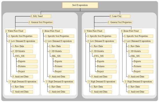
Figure 1. File structure of the folders containing data.

Table 1 gives a summary of the dataset variables in the folders. The “1. Specific Soil Properties” contains data used to determine soil characteristics that were dependent on the pore-fluid, namely, liquid limit test, plastic limit test, and soil suction tests. The “2. Low Demand Evaporation” folder contains three sub-folders. In “1. Raw Data” there are two data files that were generated during evaporation testing, including air temperature, humidity, pressure, and total mass change. In “2. 3D Models” are individual sub-folders for each model that includes a folder of exported data files, a folder that contains all the pictures captured of the sample, and a folder that holds all of the project files used to construct the 3D model. In “3. Analyzed Data” are three data files that combine raw atmospheric data, evaporation data, and soil data, respectively. The “3. High Demand Evaporation” folder contains two sub-folders. The “1. Raw Data” contains eight separate files that were developed during testing, namely, air pressure, air temperature and humidity (four datasets at four sensor locations), air velocity, surface temperature, and sample weight. The analyzed folder contains one data file that combines all of the data in a single dataset.

Table 1. Description of the dataset variables in the Prairie Climate folder.

Variable	Units	Description
General Soil Property Folder
Hydrometer
Time	min	Time format in decimal minutes.
R	cm	Measured hydrometer reading.
Rcp	cm	Corrected hydrometer reading.
Percent Finer	%	Fraction of soil finer than corresponding grain size.
Pt	%	Combined fraction of soil finer than corresponding grain size.
RcL	cm	Corrected reading for the determination of effective length.
L	cm	Effective length of hydrometer from water surface.
A		Calculation variable for diameter.
D	mm	Soil particle diameter.
T	°C	Measured temperature reading.
Ft	cm	Temperature correction to the measured reading.
Fm	cm	Meniscus correction to the measured reading.
Fz	cm	Zero correction to accommodate deflocculating agent.
a		Correction for specific gravity.
Gs		Specific gravity.
n	g∙s/cm2	Water viscosity.
Specific Gravity
Flask + Water	g	Mass of flask and water.
Flask + Water + Soil	g	Mass of flask, water, and soil.
Pan	g	Mass of pan.
Pan + Soil	g	Mass of pan and dry soil.
Soil	g	Mass of soil.
Equal Mass	g	Mass of equal volume of water as the soil solids.
Gs		Specific gravity.
Wet Sieve
Sieve No.		Sieve designation.
G	mm	Grain size.
Pan	g	Mass of pan.
Pan + Soil	g	Total of pan and dried, retained soil.
Soil	g	Mass of soil.
Retained Soil	%	Percentage of soil retained on pan.
Cumulative Retained Soil	%	Cumulative percentage of soil retained on pans.
Percent Finer	%	Fraction of soil finer than corresponding grain size.
Specific Soil Property Folder
Liquid Limit
Pan No.		The pan used for the test.
Pan	g	Mass of the pan.
Mpws	g	Mass of pan and wet soil.
Mpds	g	Mass of pan and dry soil.
w	%	Measured moisture content.
N		Number of blows.
Ms	g	Initial dry soil mass.
Mw	g	Initial fluid mass.
Plastic Limit
Pan No.		The test numbers.
Pan	g	Mass of the pan.
Pan + Wet Soil	g	Mass of pan and wet soil.
Pan + Dry Soil	g	Mass of pan and dry soil.
w	%	Measured moisture content.
Diameter	mm	Smallest diameter.
Dry Soil	g	Initial dry soil mass.
Fluid	g	Initial fluid mass.
Soil Suction
Tc	g	Mass of container at room temperature.
M1	g	Mass of container and wet filter paper.
M2	g	Mass of container and dry filter paper.
Th	g	Mass of container after removed from oven.
Mf	g	Mass of dry filter paper.
Mw	g	Mass of water in filter paper.
Wf	%	Filter paper water content.
S	Log10 kPa	Soil suction, original units.
TS	kPa	Soil suction, converted units.
w	%	Gravimetric water content of the prepared soil.
Low Demand Evaporation Folder
Raw Data: Air Temperature, Humidity, Pressure
Index		Measurement counter.
Date		Date format in DD/MM/YYYY
Time		Time format in HH:MM:SS
°C	°C	Measured air temperature.
%RH	%	Measured relative humidity.
hPa	hPa	Measured air pressure.
Raw Data: Total Mass Change
Column A		Date format in DD.MM.YYYY
Column B		Time format in HH:MM:SS
Column C	g	Measured sample weight
3D Models: Exports
File 1		Cup mesh, the raw 3D soil sample model.
File 2		Precise crop ring, used to extract the soil surface.
Pictures
All files		Digital images used to construct the 3D models.
3D Models: Project
File 1		Agisoft Metashape project file.
File 2		Ancillary project data folder.
Analyzed Data: Atmospheric Data
Time		Time format in HH:MM:SS AM/PM.
Count		Measurement counter.
Minutes		Time format in M.MM.
Hours		Time format in H.HHH.
Air Pressure	Pa	Measured air pressure.
Relative Humidity	%	Measured relative humidity.
Air Density	g/m3	Calculated air density.
Vapor Density	g/m3	Calculated absolute humidity.
Partial Vapor Pressure	Pa	Calculated partial vapor pressure.
Air Saturated Vapor Pressure	Pa	Calculated atmospheric saturated vapor pressure.
Deficit Vapor Pressure	Pa	Calculated atmospheric vapor pressure deficit.
Gradient Vapor Pressure	Pa	Calculated vapor pressure gradient.
Dew Point Temperature	°C	Calculated dew point temperature.
Mole Fraction Water Vapor		Calculated mole fraction of water vapor.
Enhancement Factor		Calculated enhancement factor of water vapor.
Compressibility Factor		Calculated compressibility factor of water vapor.
Air Temperature	°C	Measured air temperature at the indicated thermometer location.
Air Emissivity		Calculated longwave emissivity of the atmosphere above the sample.
Incoming Longwave Radiant Heat Flux	W/m2	Calculated incoming infrared radiant energy.
Analyzed Data: Evaporation Data
Date		Time format in DD.MM.YYYY.
Clock		Time format in HH:MM:SS.
Clock Hour	h	Time format in HH.
Clock Minute	min	Time format in MM.
Clock Second	s	Time format in SS.
Count		Measurement counter.
Seconds	s	Total seconds.
Mass	g	Measured mass.
Mass Difference	g	Change in mass since previous reading.
Mass Change	g	Change in mass over time.
Mass Flux	g/s∙m2	Change in mass over time, considering exposed surface area.
Measured Surface Area	cm2	Measured exposed surface area.
Analyzed Data: Soil Data
No.		3D model test number.
Time		Planned test time; time format HH.
Date		Date of test; time format MMMM, DD, HH
Time		Actual test time; time format HH.H
Avg. Total Mass	g	Average total measured mass during 3D modelling session.
Soil Mass	g	Mass of oven-dried soil.
Cup Mass	g	Mass of the container.
Fluid Mass	g	Calculated mass of the fluid in the sample.
Total Volume	cm3	Volume of the soil and fluid.
Soil Volume	cm3	Calculated volume of the soil.
Top Surface Area	cm2	Exposed surface area on the top of the soil sample.
Side Surface Area	cm2	Exposed surface area on the side of the soil sample.
Total Surface Area	cm2	Total exposed surface area.
Volume of Fluid	cm3	Calculated volume of the fluid.
Volume of Voids	cm3	Calculated volume of the voids.
Void Ratio		Calculated ratio of the void volume to soil volume.
Saturation	%	Calculated saturation.
Volumetric Water Content	%	Calculated volumetric water content.
Gravimetric Water Content	%	Calculated gravimetric water content.
Axial Length	mm	Vertical length of the soil sample.
Radial Length X	mm	X-axis horizontal length of the soil sample.
Radial Length Y	mm	Y-axis horizontal length of the soil sample
Radial Length Avg.	mm	Average horizontal length of the soil sample.
Surface Area Deformation	%	Change in surface area since first measurement.
Total Volume Deformation	%	Change in total volume since first measurement.
Axial Deformation	%	Change in vertical length since first measurement.
Radial Deformation	%	Change in horizontal length since first measurement.
Raw Data: Air Pressure
Index		Measurement counter.
Date		Date format in DD/MM/YYYY
Time		Time format in HH:MM:SS
°C	°C	Measured air temperature at the barometer location.
%RH	%	Measured relative humidity at the barometer location.
hPa	hPa	Measured air pressure at the barometer location.
Pa	Pa	Converted air pressure value.
High Demand Evaporation Folder
Raw Data: Air Temperature-Air Humidity
No.		Measurement counter.
Time		Time and date format in YYYY-MM-DD HH:MM:SS
Temperature	°C	Measured air temperature at the indicated thermometer location.
Humidity	%	Measured relative humidity at the indicated hygrometer location.
Raw Data: Air Velocity
Index		Measurement counter.
Time		Time format in HH:MM:SS
Wind Value	m/s	Measured air velocity at the anemometer location.
Temp	°C	Measured air temperature at the anemometer location.
Raw Data: Surface Temperature
Data Point		Measurement counter.
Log Date		Date format in YYYY-MM-DD
Log Time		Time format in HH:MM:SS AM/PM
°C	°C	Measured sample surface temperature.
Raw Data: Weight
Column A		Date format in DD.MM.YYYY
Column B		Time format in HH:MM:SS
Column C	g	Measured sample weight.
Analyzed Data: Data Summary
Time		Time format in HH:MM:SS AM/PM.
Count		Measurement counter.
Minutes		Time format in M.MM.
Hours		Time format in H.HHH.
Velocity	m/s	Measured air velocity at the anemometer location.
Aerodynamic Resistance	s/m	Calculated aerodynamic resistance.
Air Pressure	Pa	Measured air pressure at the barometer location.
Air Pressure Interpolated	Pa	Calculated air pressure at 10 s intervals using linear equation between 30 s intervals.
Psychrometric Constant	Pa/°C	Calculated psychrometric constant.
Relative Humidity	%	Measured relative humidity at the indicated hygrometer location.
Air Density	g/m3	Calculated air density.
Vapor Density	g/m3	Calculated absolute humidity.
Partial Vapor Pressure	Pa	Calculated partial vapor pressure.
Air Saturated Vapor Pressure	Pa	Calculated atmospheric saturated vapor pressure.
Deficit Vapor Pressure	Pa	Calculated atmospheric vapor pressure deficit.
Gradient Vapor Pressure	Pa	Calculated vapor pressure gradient.
Dew Point Temperature	°C	Calculated dew point temperature.
Mole Fraction Water Vapor		Calculated mole fraction of water vapor.
Enhancement Factor		Calculated enhancement factor of water vapor.
Compressibility Factor		Calculated compressibility factor of water vapor.
Incoming Shortwave Radiant Heat Flux	W/m2	Calibrated incoming solar irradiance.
Air Temperature	°C	Measured air temperature at the indicated thermometer location.
Air Emissivity		Calculated longwave emissivity of the atmosphere above the sample.
Incoming Longwave Radiant Heat Flux	W/m2	Calculated incoming infrared radiant energy.
Sample Mass Measured	g	Measured sample mass.
Sample Mass Interpolated	g	Calculated sample mass using a polynomial regression
Sample Mass Rate of Change	g/s	Calculated change in sample mass using.
Air Saturated Water Density	g/m3	Calculated air saturated density of water.
Isothermal Compressibility		Calculated isothermal compressibility.
Corrected Water Density	g/m3	Calculated corrected water density.
Sample Volume	m3	Calculated sample volume.
Sample Surface Area	m2	Calculated sample surface area.
Surface Saturated Vapor Pressure	Pa	Calculated atmospheric saturated vapor pressure.
Total Vapor Flux	g/s ∙m2	Calculated evaporative flux.
Evaporation Rate	mm/day	Calculated rate of evaporation.
Outgoing Shortwave Radiant Heat Flux	W/m2	Measured outgoing solar irradiance.
Corrected Outgoing Shortwave Radiant Heat Flux	W/m2	Corrected outgoing solar irradiance.
Surface Temperature	°C	Measured sample surface temperature.
Outgoing Longwave Radiant Heat Flux	W/m2	Calculated outgoing infrared radiant energy.
Net Radiant Heat Flux	W/m2	Calculated net radiant heat flux at the surface.
Bowen Ratio		Calculated Bowen Ratio.
Sensible Thermal Heat Flux	W/m2	Calculated atmospheric thermal heat flux.
Conductive Thermal Heat Flux	W/m2	Calculated ground heat flux.
Available Energy	W/m2	Calculated available energy.
Evaporative Latent Heat	J/g	Calculated evaporative latent heat energy.
Evaporative Latent Heat Flux	W/m2	Calculated evaporative latent heat flux.
Evaporative Latent Heat Flow	W	Calculated evaporative latent heat flow.

3. Methodology

3.1. Soil Selection and Retrieval

The Canadian Soil Information Service (CanSIS) database contains water retention data for soils in the form of volumetric water content (θ) at critical matric suction values. Generally, regional soils range from sandy loam to clayey loam with variable amounts of sand (2.0–0.5 mm), silt (0.5–0.002 mm), and clay (<0.002 mm). To appreciate the range of agricultural soils, 25 irrigation districts from across southern Saskatchewan (Figure 2) were analyzed. These districts are in the form of variably shaped polygons, as delineated by the Saskatchewan Irrigation District Map (SIDM). The CanSIS and SIDM databases were merged to extract the weighted average values of θ and grain sizes for each district; the latter were converted to the Unified Soil Classification System (USCS) using [9]. Figure 3 gives the θ values corresponding to various soils in the irrigation districts. Regional soils range from silty sands (SM) to lean clays (CL) with θ varying as follows: 43–54% at 0 kPa, 15–45% at 33 kPa, and 8–27% at 1500 kPa. The selected soils, namely, silty sand (SM) from Avonlea [10] and a lean clay (CL) from Belle Plain [11], had θ values within the above ranges [6].

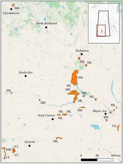
Figure 2. Saskatchewan irrigation districts and weighted average USCS classifications.

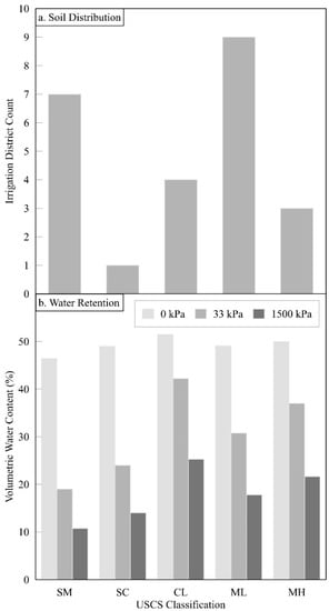
Figure 3. Soil characterization of irrigation districts: (a) soil distribution and (b) water retention.

Representative soil samples were retrieved using a shovel, sealed in plastic bags to preclude impurities, and preserved in 20 L buckets. Soils were brought to and stored at the Advanced Geotechnical Testing Laboratory at the University of Regina following the Standard Practices for Preserving and Transporting Soil Samples (ASTM D4220/D4220M-14).

3.2. Pore Fluid Selection

The pore fluids were classified as “non-saline” and “very saline” in accordance with the salinity classes for agricultural soils, as defined by [12]. The non-saline fluid was essentially distilled water that contained less than 10 ppm of dissolved salts. In contrast, the saline fluid was prepared by mixing 1 L of distilled water with 5.50 g of NaCl and stirring until all of the solids had completely dissolved [7]. Based on molarity (0.15 M), the saline solution represented a pore fluid that would cause significant yield decrease [13].

3.3. General Soil Properties

The soils were classified as per the Standard Practice for Classification of Soils for Engineering Purposes (Unified Soil Classification System) (ASTM D2487-17). For this purpose, the general soil properties tests were conducted using distilled water. Located in “1. General Soil Properties”, the folders contain data for the following analyses: (i) wet sieve, (ii) hydrometer, and (iii) specific gravity. These tests are needed in part for classifying soils under the USCS and calculating various geotechnical parameters [14].

The wet sieve analysis was performed to determine the soil portion greater than 0.002 mm. The tests were conducted following the Standard Test Methods for Particle Size Distribution (Gradation) of Soils Using Sieve Analysis (ASTM D6913/D6913M-17). The stack included sieve numbers 4, 10, 20, 40, 60, 120, and 200 as well as a bottom container to collect material finer than 0.075 mm. The measured pan weight ($M_{se}$; g) pertained to the empty sieves and the measured total weight ($M_{st}$; g) was that of the sieve and the retained soil after oven drying. The soil weight ($M_{ss}$; g) retained in each sieve was calculated according to the following equation:

$$M_{ss}=M_{st}-M_{se}$$

(1)

The percent retained ($P{R}_s$; %) on each sieve and the pan was calculated from the soil weight ($M_{ss}$; g) (Equation (1)) and the total weight ($M_{sf}$; g), which was the sum total of all retained soil weights, using the following equation:

$$P{R}_s=\frac{M_{ss}}{M_{sf}}$$

(2)

The percent finer ($P{F}_s$; %) was calculated using cumulative percent retained ($CP{R}_s$; %), which was the cumulative sum of percent retained ($P{R}_s$; %) (Equation (2)) in the following equation:

$$P{F}_s=1-CP{R}_s$$

(3)

The percent lost ($P{T}_s$; %) was the amount of soil unaccounted for during the sieving process and was calculated as follows:

$$P{T}_s=1-\frac{M_{sf}}{M_{si}}$$

(4)

The hydrometer analysis was performed to determine the soil portion less than 0.002 mm. The tests were conducted following the Standard Test Method for Particle Size Distribution (Gradation) of Fine-Grained Soils Using the Sedimentation (Hydrometer) Analysis (ASTM D7928-21). Fourteen data points at pre-determined times were collected over 48 h. The hydrometer reading ($R_h$; mm) was measured at the top of the meniscus and was adjusted by the corrected hydrometer reading ($R_{cp}$; mm) using temperature correction ($F_t$; mm) (Equation (6)) and the measured zero correction ($F_z$; mm) in the equation:

$$R_{cp}=R_h+F_t-F_z$$

(5)

The temperature correction was an adjustment required because the test may not have occurred at exactly 20 °C water and was calculated using measured water temperature ($T$; °C) in the equation:

$$F_t=-4.85-0.25·T$$

(6)

The percent finer ($P{F}_h$; %) was calculated using the measured dry soil weight ($W_{sh}$; g), corrected hydrometer reading ($R_{cp}$; mm) (Equation (5)) and specific gravity correction ($a_s$) (Equation (8)) in the equation:

$$P{F}_h=\frac{a_s·R_{cp}}{W_{sh}}·100$$

(7)

The specific gravity correction ($a_s$) was an adjustment required because the hydrometer was calibrated for a specific gravity value of 2.65, and calculated using the measured specific gravity ($G_s$) in equation [14]:

$$a_s=\frac{G_s·1.65}{\left(G_s-1\right)·2.65}$$

(8)

The combined percent finer ($CP{F}_h$; %) was calculated using the percent finer ($P{F}_h$; %) (Equation (7)) and the percent finer than the number 200 sieve ($P{F}_{s200}$; %) (Equation (3)) in the equation:

$$CP{F}_h=P{F}_h·\frac{P{F}_{s}200}{100}$$

(9)

The grain size ($D_h;$ mm) was calculated using the adjustment factor ($A_h$) (Equation (11)), the effective length ($L_h$; cm) (Equation (13)), and the measured time ($t_h$; min) in the equation:

$$D_h=A_h·\sqrt{\frac{L_h}{t_h}}$$

(10)

The adjustment factor ($A_h$) was calculated using the viscosity of water ($\eta$; g∙s∙cm⁻²) (Equation (12)) and the measured specific gravity ($G_s$) in the equation:

$$A_h=\sqrt{\frac{30·\eta }{\left(G_s-1\right)}}$$

(11)

The viscosity of water ($\eta$; g∙s/cm²) was calculated using the measured temperature of water ($T_h$; °C) in the equation:

$$\eta =\frac{\left(2.414·{10}^{-5}\right)·\left({10}^{\frac{247.8}{\left(T_h+273.15\right)-140}}\right)}{100}$$

(12)

The effective length ($L_h$; cm) pertains to the settling zone of soil particles with a known diameter in a given time. The length was calculated using the corrected reading for determination of effective length ($R_{cl}$; cm) (Equation (14)) in the equation:

$$L_h=10.5-\frac{10.5-2.3}{50}·R_{cl}+0.5·14-\frac{67}{27.7}$$

(13)

The corrected reading for determination of effective length ($R_{cl}$; cm) was calculated using the hydrometer measurement ($R_h$; mm) and meniscus correction measurement ($F_z$; mm) in the equation:

$$R_{cl}=R_h+F_z$$

(14)

The specific gravity ($G_s$) tests were conducted following the Standard Test Methods for Specific Gravity of Soil Solids by Water Pycnometer (ASTM D854-14). Three replicate samples were tested, and the values were averaged. Specific gravity was calculated using the mass of soil ($M_{gs}$; g) (Equation (16)) and the mass of equal volume of water as the soil solids ($M_{gswp}$; g) (Equation (17)) in the equation:

$$G_s=\frac{M_{gs}}{M_{gswp}}$$

(15)

The mass of soil ($M_{gs}$; g) was calculated using the measured mass of empty pan ($M_{gp}$; g) and the mass of the pan and oven-dried soil together ($M_{gsp}$; g) in the equation:

$$M_{gs}=M_{gp}+M_{gsp}$$

(16)

The mass of equal volume of water as the soil solids ($M_{gswp}$; g) was calculated using the measured mass of the flask and water ($M_{gfw}$; g), mass of the flask, water and soil ($M_{gfws}$; g), and mass of soil ($M_{gs}$; g) (Equation (15)) in the equation:

$$M_{gswp}=\left(M_{gfw}+M_{gs}\right)-M_{gfw}$$

(17)

3.4. Specific Soil Properties

The specific soil properties include tests that were affected by pore fluid salinity. Located in “1. Specific Soil Properties”, the folders contain data for the following analyses: (i) liquid limit, (ii) plastic limit, and (iii) water retention. These tests were needed for classifying soils under the USCS and understanding soil behavior.

The liquid limit and the plastic limit analyses were performed to determine the gravimetric water contents at which the soil transitioned from liquid-to-plastic and plastic-to-semi-solid states, respectively. The tests were conducted following the Standard Test Methods for Liquid Limit, Plastic Limit, and Plasticity Index of Soils (ASTM D4318-17e1). Three tests were performed for each analysis to develop linear relation between water content (Equation (18)) and measured number of blows ($N_L$) for liquid limit. The liquid limit ($LL$; %) water content corresponds to 25 blows ($N=25$). Three tests were performed to obtain a diameter ($D_P=3.18 \mathrm{mm}$) of a soil thread without crumbling for plastic limit ($PL$; %). In both cases, water content ($w_A$; %) was calculated using the measured mass of empty pan ($M_{Ap}$; g), measured mass of the pan and oven-dried soil together ($M_{Asp}$; g), and measured mass of the pan and wetted soil together ($M_{Aspw}$; g) in the equation:

$$w_A=\frac{M_{Aspw}-M_{Asp}}{M_{Asp}-M_{Ap}}$$

(18)

Soil suction was determined following the Standard Test Method for Measurement of Soil Potential (Suction) using Filter Paper (ASTM D5298-16) through the Whatman No. 42 filter paper for simultaneous measurement of total and matric suction [15]. Details on the preparation steps are given by [6]. The bi-linear calibration curve (developed by Greacen et al. [16] and endorsed by ASTM) was used to ensure data accuracy [17]. The wetting and drying suction tests were both performed beginning with 100 g of oven-dried soil in ten separate glass jars. Wetting suction tests had between 1 g to 37 g of fluid (distilled or saline) added to achieve target gravimetric water contents ranging from 1% to 37%, in four percent increments. In contrast, drying suction tests had 38 g of fluid added and then sealed for 24 h to allow homogenization. The samples were allowed to desiccate under the ambient laboratory environment (with a measured temperature of 19.6 ± 0.4 °C and relative humidity of 21.7 ± 6.5%) until the target gravimetric water contents were achieved. The wetting and drying samples were then stored inside an insulated box for 30 days to ensure equilibration of filter paper for water content. Afterward, each jar was opened to measure the water content in the filter paper ($w_f$; %) using the mass of filter paper ($M_f$; g) (Equation (20)) and the mass of filter paper water ($M_w$; g) (Equation (21)) in the equation:

$$w_f=\frac{M_w}{M_f}·100$$

(19)

The mass of filter paper ($M_f$; g) was calculated using mass measurements of the oven-dried filter paper and the warm metal container together ($M_2$; g) and the warm metal container alone ($T_h$; g) in the equation:

$$M_f=M_2-T_h$$

(20)

The mass of filter paper water ($M_w$; g) was calculated using mass measurements of the cold metal container alone ($T_c$; g), wet filter paper and cold metal container together ($M_1$; g), oven-dried filter paper and warm metal container together ($M_2$; g) and the warm metal container alone ($T_h$; g) in the equation:

$$M_w=M_1-M_2-T_c+T_h$$

(21)

3.5. Low Demand Evaporation

The low-demand evaporation tests were performed under ambient laboratory conditions, continuously capturing water loss from the soil and intermittently capturing 3D model information. Located in “3. Analyzed Data” of “2. Low Demand Evaporation”, the folders contain data for the following analyses: (i) atmosphere, (ii) evaporation, and (iii) soil. These tests were needed to study the interactions that occur between evaporation and the types of soil and pore fluids.

The atmospheric analyses were performed to characterize atmospheric conditions above the evaporating surfaces. Atmospheric measurements taken at 30 s intervals included pressure ($e_a$; Pa), relative humidity ($h$; %), and temperature ($T_a$; °C). Air density (${\rho }_a$; g∙m⁻³) was calculated using air pressure ($e_a$; Pa), air temperature ($T_{aul}$; °C), molar mass of dry air ($M_a$; 28.96546 g∙mol⁻¹), molar mass of water ($M_v$; 1.801528 g∙mol⁻¹), molar gas constant ($R$; 8.314472 J∙mol⁻¹∙°K⁻¹), mole fraction of water vapor ($x_v$) (Equation (23)) and compressibility factor ($Z$) (Equation (25)) with the following equation [18]:

$${\rho }_a=\frac{P·M_a}{Z·R·(T_a+273.15)}·\left[1-x_v\left(1-\frac{M_v}{M_a}\right)\right]$$

(22)

The mole fraction of water ($x_v$) was calculated using air pressure ($e_a$; Pa), relative humidity ($h$; %), enhancement factor ($f$) (Equation (24)), and saturated vapor pressure ($e_s$; Pa) (Equation (28)) with the equation [18]:

$$x_v=h·f·\left(\frac{e_s}{P_i}\right)$$

(23)

The enhancement factor ($f$) was calculated using air temperature ($T_a$; °C), air pressure ($e_a$; Pa), and the constants $A$ (1.00062), $B$ (3.14 × 10⁻⁸ Pa⁻¹), and $C$ (5.6 × 10⁻⁷ °C⁻²) with the equation [18]:

$$f=A+B·P+C·T_a^2$$

(24)

The compressibility factor ($Z$) was calculated using air temperature ($T_a$; °C), air pressure ($e_a$; Pa), mole fraction of water ($x_v$) and the constants $a_0$ (1.58123 × 10⁻⁶ °K∙Pa⁻¹), $a_1$ (−2.9331 × 10⁻⁸ Pa⁻¹), $a_2$ (1.1043 × 10⁻¹⁰ °K⁻¹∙Pa⁻¹), $b_0$ (5.707 × 10⁻⁶ °K∙Pa⁻¹), $b_1$ (−2.051 × 10⁻⁸ Pa⁻¹), $c_0$ (1.9898 × 10⁻⁴ °K∙Pa⁻¹), $c_1$ (−2.376 × 10⁻⁶ Pa⁻¹), $d_0$ (1.83 × 10⁻¹¹ °K²∙Pa⁻²), and $e_0$ (−0.765 × 10⁻⁸ °K²∙Pa⁻²), with the equation [18]:

$$\begin{gathered} Z=1-\frac{P_i}{T_a+273.15}·\left[a_0+a_1·T_a+a_2·T_a^2+\left(b_0+b_1·T_a\right)·x_v+\left(c_0+c_1·T_a\right)·x_v^2\right]+ \\ \frac{P_i^2}{{\left(T_a+273.15\right)}^2}·\left(d_0+e_0·x_v^2\right) \end{gathered}$$

(25)

The partial vapor pressure ($e_a$; Pa), the force per unit area exerted by gas-state water in the atmosphere, was calculated at each atmospheric point using dew point temperature ($T_d$; °C) (Equation (27)) [19]:

$$e_a=61.08·\exp \left(\frac{17.27·T_d}{T_d+237.3}\right)$$

(26)

The dew point temperature ($T_d$; °C) was calculated using relative humidity ($h$; %) and air temperature ($T_a$; °C) with the equation [19]:

$$T_d=\frac{237.3\left(\frac{\ln \left(h/100\right)}{17.27}+\frac{T_a}{237.3+T_a}\right)}{1-\left(\frac{\ln \left(h/100\right)}{17.27}+\frac{T_a}{237.3+T_a}\right)}$$

(27)

The saturated vapor pressure ($e_s$; Pa), air temperature at which water vapor is in equilibrium with the surface boundary of liquid water, was calculated using air temperature ($T_a$; °C) with the equation [20]:

$$e_s=61.08·\exp \left(\frac{17.27·T_{a or s}}{237.3+T_{a or s}}\right)$$

(28)

The vapor pressure deficit ($e_d$; Pa), capacity in the atmosphere for water vapor to enter from the surface boundary of liquid water, was calculated at each atmospheric point using partial vapor pressure ($e_a$; Pa) (Equation (26)) and saturated vapor pressure ($e_s$; Pa) (Equation (28)) with the equation [21]:

$$e_d=e_s-e_a$$

(29)

The vapor density (${\rho }_v$; g∙m⁻³), mass per unit volume of water vapor in the climate chamber atmosphere, was calculated at each atmospheric point air temperature ($T_a$; °C) and partial vapor pressure ($e_a$; Pa) (Equation (26)) with the equation [19]:

$${\rho }_v=\frac{2165·e_a}{1000·\left(T_a+273.15\right)}$$

(30)

The vapor pressure gradient ($\Delta$; Pa∙°C⁻¹), gradient of the saturated vapor pressure function, and was calculated using saturated vapor pressure ($e_s$; Pa) (Equation (28)) and measured air temperature ($T_a$; °C) [20]:

$$\Delta =\frac{e_s·4098}{{\left(234.3+T_a\right)}^2}$$

(31)

The incoming longwave irradiation ($L_i$; W∙m⁻²) was calculated using air temperature ($T_a$; °C), air emissivity (${\epsilon }_a$) (Equation (33)), and the Stefan–Boltzmann constant ($\sigma$; 5.670∙10⁻⁸ W∙m⁻²∙°C⁻⁴) with the equation [22]:

$$L_i={\epsilon }_a·\sigma ·{\left(T_a+273.15\right)}^4$$

(32)

The air emissivity (${\epsilon }_a$) was calculated using air temperature ($T_a$; °C) and partial vapor pressure ($e_a$; Pa) (Equation (26)) with the equation [23]:

$${\epsilon }_a=0.7+5.95e^{-5}·\left(\frac{e_a}{100}\right)·\exp \left(\frac{1500}{273.15+T_a}\right)$$

(33)

The evaporation analyses were performed to characterize the evaporative flux conditions occurring at the surface. Evaporative flux ($\mathsf{\Phi }$; g∙s⁻¹∙m⁻²) was calculated using change in measured mass ($\mathsf{\Delta }M$; g∙s⁻¹) (Equation (35)) and average surface area ($SA$; cm²) (Equation (36)) with the equation:

$$\mathsf{\Phi }=\mathsf{\Delta }M·\frac{1}{\frac{SA}{10,000}}$$

(34)

The change in measured mass ($\mathsf{\Delta }M$; g∙s⁻¹) was calculated using mass measurements during 3D model captured in the CPS at time point one ($M_1$; g) and time point two ($M_2$; g), in the equation:

$$\mathsf{\Delta }M=M_2-M_1$$

(35)

The average surface area ($S{A}_A$; cm²) was calculated using total surface area measurements (Equation (41)) at time point one ($S{A}_1$; cm²) and time point two ($S{A}_2$; cm²) in the equation:

$$S{A}_A=\frac{\left(S{A}_1+S{A}_2\right)}{2}$$

(36)

The soil analyses were performed to characterize the soil conditions below the evaporating surface. The fluid mass ($M_{sf}$; g) was calculated using mass measurements of the total sample ($M_{st}$; g), oven-dried soil ($M_{ss}$; g), and sample cup ($M_{sc}$; g) in the equation:

$$M_{sf}=M_{st}-M_{ss}-M_{sc}$$

(37)

The volume of soil ($V_s$; cm³) was calculated using measurements of oven-dried soil mass ($M_{ss}$; g) and the specific gravity of the soil ($G_s$) (Equation (15)) in the equation:

$$V_s=\frac{M_{ss}}{G_s}$$

(38)

The volume of fluid ($V_f$; cm³) was calculated using fluid density (${\rho }_f$; g∙cm⁻³), total sample mass ($M_{st}$; g), oven-dried soil mass ($M_{ss}$; g), and sample cup mass ($M_{sc}$; g) in the equation:

$$V_f=\frac{M_{st}-\left(M_{ss}+M_{sc}\right)}{{\rho }_f}$$

(39)

The volume of voids, ($V_v$; cm³) was calculated using volume of soil ($V_s$; cm³) (Equation (38)) and measured sample volume ($V_t$; cm³) obtained from 3D models in the equation:

$$V_v=V_t-V_s$$

(40)

The total surface area ($SA$; cm²) was calculated using measurements of the top surface area ($S{A}_{to}$; cm²) and the side surface area ($S{A}_{si}$; cm²) in the equation:

$$SA=S{A}_{to}+S{A}_{si}$$

(41)

The void ratio ($e$) was calculated using volume of soil ($V_s$; cm³) (Equation (38)) and the volume of voids ($V_v$; cm³) (Equation (40)) in the equation:

$$e=\frac{V_v}{V_s}$$

(42)

The degree of saturation ($S$; %) was calculated using specific gravity ($G_s$) (Equation (15)), void ratio ($e$) (Equation (42)) and gravimetric water content ($w$; %) (Equation (45)) in the equation:

$$S=\frac{e·G_s}{w}$$

(43)

The volumetric water content ($\theta$; %) was calculated using fluid density (${\rho }_f$; g∙cm⁻³), specific gravity ($G_s$) (Equation (15)), void ratio ($e$) (Equation (42)) and gravimetric water content ($w$; %) (Equation (45)) in the equation:

$$\theta =\frac{\frac{G_s}{e+1}·w}{w}$$

(44)

The gravimetric water content ($w$; %) was calculated using total sample mass ($M_{st}$; g), oven-dried soil mass ($M_{ss}$; g), and sample cup mass ($M_{sc}$; g) in the equation:

$$w=100·\frac{M_{st}-\left(M_{ss}+M_{sc}\right)}{M_{ss}}$$

(45)

The surface area deformation ($D_s$; %), the ratio of surface area (Equation (41)) at time ($S{A}_t$; cm²) to the initial exposed area at 0 h ($S{A}_o$), was calculated in the equation:

$$D_s=-100·\left(1-\frac{S{A}_t}{S{A}_o}\right)$$

(46)

The volume deformation ($D_v$; %), the ratio of measured total volume by 3D model at time ($V_{tt}$; cm³) to the initial volume at 0 h ($V_{t0}$), was calculated in the equation:

$$D_v=100·\left(1-\frac{V_{tt}}{V_{to}}\right)$$

(47)

The axial deformation ($D_h$; %), the ratio of measured 3D model height at time ($H_t$; cm) to the initial height at 0 h ($H_0$), was calculated in the equation:

$$D_h=100·\left(1-\frac{H_t}{H_o}\right)$$

(48)

The radial deformation ($D_d$; %), the ratio of average 3D model diameter (Equation (50)) at time ($D_t$; cm) to the initial diameter at 0 h ($D_0$), was calculated in the equation:

$$D_d=100·\left(1-\frac{D_t}{D_o}\right)$$

(49)

The radial diameter ($D$; cm) was calculated using measured diameter on the 3D model in the X ($D_x$; cm) and Y ($D_y$; cm) Cartesian coordinate directions in the equation:

$$D=\frac{D_x+D_y}{2}$$

(50)

3.6. High Demand Evaporation

The high-demand evaporation experiments were performed under Canadian Prairie summer day conditions [24], continuously capturing water loss from the soil. Located in “3. Analyzed Data” of “2. High Demand Evaporation”, the folders contain data for atmosphere and evaporation in the “Data Summary” file. The high-demand tests include surface atmosphere information in addition to Equations (22) to (50) for integration into prediction models, which are described in detail by [8].

References

- Roberts, K.; Cahill, C.; Soulard, F.; Wang, J.; Henry, M.; Gagnon, G. Human Activity and the Environment: Freshwater in Canada; Catalogue no. 16 201 X; Statistics Canada: Ottawa, ON, Canada, 2017. [Google Scholar]
- Lemmen, D.S.; Vance, R.E.; Campbell, I.A.; David, P.P.; Pennock, D.J.; Sauchyn, D.J.; Wolfe, S.A. Geomorphic Systems of the Palliser Triangle, Southern Canadian Prairies: Description and Response to Changing Climate; Geological Survey of Canada: Ottawa, ON, Canada, 1998. [Google Scholar] [CrossRef]
- Pennock, D.J.; De Jong, E. Spatial pattern of soil redistribution in boreal landscapes, southern Saskatchewan, Canada. Soil Sci. 1990, 150, 867–873. [Google Scholar] [CrossRef]
- Teller, J.T.; Moran, S.R.; Clayton, L. The Wisconsinan deglaciation of southern Saskatchewan and adjacent areas: Discussion. Can. J. Earth Sci. 1980, 17, 539–541. [Google Scholar] [CrossRef]
- Trenberth, K.E. Changes in precipitation with climate change. Clim. Res. 2011, 47, 123–138. [Google Scholar] [CrossRef]
- Suchan, J.; Azam, S. Influence of desaturation and shrinkage on evaporative flux from Soils. Geotechnics 2022, 2, 412–426. [Google Scholar] [CrossRef]
- Suchan, J.; Azam, S. Influence of saline pore fluid on soils behavior during evaporation. Geotechnics 2022, 2, 754–764. [Google Scholar] [CrossRef]
- Suchan, J.; Azam, S. Datasets for the determination of evaporative flux from distilled water and saturated brine using bench-scale atmospheric simulators. Data 2021, 7, 1. [Google Scholar] [CrossRef]
- García-Gaines, R.; Frankenstein, S. USCS and the USDA Soil Classification System: Development of a Mapping Scheme; U.S. Army Engineer Research and Development Center: Vicksburg, MS, USA, 2015. [Google Scholar]
- Azam, S.; Khan, F. Geohydrological properties of selected badland sediments in Saskatchewan, Canada. Bull. Eng. Geol. Environ. 2013, 73, 389–399. [Google Scholar] [CrossRef]
- Paranthaman, R.; Azam, S. Effect of composition on engineering behavior of clay tills. Geosciences 2021, 11, 427. [Google Scholar] [CrossRef]
- Dahnke, W.C.; Whitney, D.A. Measurement of Soil Salinity; North Dakota Agricultural Experiment Station: Fargo, ND, USA, 1988. [Google Scholar]
- Smith, J.L.; Doran, J.W. Measurement and use of pH and electrical conductivity for soil quality analysis. Methods Assess. Soil Qual. 1997, 49, 169–182. [Google Scholar]
- Das, B.M.; Sobhan, K. Principles of Geotechnical Engineering, 8th ed.; Cengage Learning: Stamford, CT, USA, 2014. [Google Scholar]
- Suits, L.D.; Sheahan, T.; Leong, E.; He, L.; Rahardjo, H. Factors affecting the filter paper method for total and matric suction measurements. Geotech. Test. J. 2002, 25, 8198. [Google Scholar] [CrossRef]
- Greacen, E.L.; Walker, G.R.; Cook, P.G. Procedure for Filter Paper Method of Measuring Soil Water Suction; CSIRO Division of Soils: Adelaide, Australia, 1987. [Google Scholar]
- Kim, H.; Prezzi, M.; Salgado, R. Calibration of whatman grade 42 filter paper for soil suction measurement. Can. J. Soil Sci. 2016, 97, 93–98. [Google Scholar] [CrossRef]
- Picard, A.; Davis, R.; Gläser, M.; Fujii, K. Revised formula for the density of moist air (CIPM-2007). Metrologia 2008, 45, 149–155. [Google Scholar] [CrossRef]
- Snyder, R.L. Humidity Conversion; University of California, Biometeorology Group: Davis, CA, USA, 2005. [Google Scholar]
- Shuttleworth, W.J. Evaporation. In Handbook of Hydrology, 1st ed.; Maidment, D.R., Ed.; McGraw-Hill Inc.: New York, NY, USA, 1993; Volume 1, pp. 4.1–4.53. [Google Scholar]
- Yuan, W.; Zheng, Y.; Piao, S.; Ciais, P.; Lombardozzi, D.; Wang, Y.; Ryu, Y.; Chen, G.; Dong, W.; Hu, Z.; et al. Increased atmospheric vapor pressure deficit reduces global vegetation growth. Sci. Adv. 2019, 5, eaax1396. [Google Scholar] [CrossRef] [PubMed]
- An, N.; Hemmati, S.; Cui, Y.-J. Assessment of the methods for determining net radiation at different time-scales of meteorological variables. J. Rock Mech. Geotech. Eng. 2017, 9, 239–246. [Google Scholar] [CrossRef]
- Idso, S.B. A set of equations for full spectrum and 8- to 14-μm and 10.5- to 12.5-μm thermal radiation from cloudless skies. Water Resour. Res. 1981, 17, 295–304. [Google Scholar] [CrossRef]
- Suchan, J.; Azam, S. Determination of evaporative fluxes using a Bench-Scale Atmosphere Simulator. Water 2021, 13, 84. [Google Scholar] [CrossRef]
Publisher’s Note: MDPI stays neutral with regard to jurisdictional claims in published maps and institutional affiliations. |
© 2022 by the authors. Licensee MDPI, Basel, Switzerland. This article is an open access article distributed under the terms and conditions of the Creative Commons Attribution (CC BY) license (https://creativecommons.org/licenses/by/4.0/).