Assessing the Accuracy of Google Trends for Predicting Presidential Elections: The Case of Chile, 2006–2021

Abstract

This article presents the results of reviewing the predictive capacity of Google Trends for national elections in Chile. The electoral results of the elections between Michelle Bachelet and Sebastián Piñera in 2006, Sebastián Piñera and Eduardo Frei in 2010, Michelle Bachelet and Evelyn Matthei in 2013, Sebastián Piñera and Alejandro Guillier in 2017, and Gabriel Boric and José Antonio Kast in 2021 were reviewed. The time series analyzed were organized on the basis of relative searches between the candidacies, assisted by R software, mainly with the gtrendsR and forecast libraries. With the series constructed, forecasts were made using the Auto Regressive Integrated Moving Average (ARIMA) technique to check the weight of one presidential option over the other. The ARIMA analyses were performed on 3 ways of organizing the data: the linear series, the series transformed by moving average, and the series transformed by Hodrick–Prescott. The results indicate that the method offers the optimal predictive ability.

1. Introduction

Chile has a system of government in which the president acts as head of state and of government. The Chilean government has three branches: executive, legislative and judicial. Based on the principles of the political system defined in Chile’s constitution, only the executive and legislative branches are elected by popular, open, and voluntary vote. However, voting has been voluntary only since 2009. The Chilean presidential system establishes that laws and regulations that require fiscal budgetary expenditure depend exclusively on the president of the republic, while other types of initiatives that arise from the legislative branch (chamber of deputies and senate) need presidential sponsorship or should not require fiscal expenditure. This reality means that presidential elections take on special relevance in defining the destiny of the nation, given that it will be the government project headed by the president in office that will determine the guidelines along which the country will advance during the four-year presidential term. In simple terms, the nation defines its roadmap every four years by deciding who will be the next president of the republic. This condition makes presidential campaigns highly intensive in terms of media demand, information flow, and civic and political interaction. The campaigns of each conglomerate usually last about 90 days, while the electoral period is close to two months. The main conglomerates are composed of two major right-wing parties: Unión Demócrata Independiente (UDI) and Renovación Nacional (RN), recently joined by Evopoli, Partido de la Gente and Republicanos. There is another center-left conglomerate composed of the Christian Democratic Party (DC), the Party for Democracy (PPD), the Radical Party (PR), and the Socialist Party (PS). Since 2017, a conglomerate of progressive left-wing parties called Frente Amplio (FA) has been strongly established, which together with the Communist Party (PC) and other progressive factions of the Socialist Party now make up a relevant political force (the current president Gabriel Boric comes from these forces). On the left, there are other groups with less electoral weight in presidential campaigns, which is what is reviewed in this article. The Chilean political landscape is currently undergoing significant structural redefinitions.

In October 2019, Chile entered a process of social revolt triggered by various reasons that stem from the degradation of democratic institutions in their ability to represent the needs of the population and the structural inequality in constant reproduction [1,2]. At a critical moment in Chile’s political history, the political class decided to initiate a constituent process to replace the constitution implemented during the dictatorship of Augusto Pinochet with a new one drafted in democracy, which would redefine a large part of the electoral map. In addition, Pinochet’s constitution had already been in force for 39 years and retained a set of locks that prevented changes in line with the social needs of the 21st century [3]. Through a transversal political agreement, a constituent process was initiated to draft a new constitutional text. With this process, the political scene is becoming more and more heated, and the 2021 presidential elections were the most widely contested voluntary elections in the country’s history. In this context of heightened civic activity, the results of this study would help to understand in part the advance of the public space where civic interaction is taking place, the virtual political space.

Google has become the main connector between questions and answers in the world, achieving significant penetration among its users. According to DataReportal, 1.2 trillion global searches are performed annually [4]. The relationship between user interest and access to information is increasingly used in different studies to identify patterns, preferences, business opportunities, and the effectiveness of business campaigns among multiple applications. It is also beginning to be used in scientific research to access data that facilitates the process of analyzing certain concepts, trends, and information flow, including the possibility of using this information to predict potential electoral results, thus awakening the interest of the public in the use of information [5]. This has awakened the political world’s interest in incorporating these monitoring and diagnostic elements into the design of campaigns. The greater the penetration of internet use in a population, the greater should be the accuracy of the electoral forecasting tools based on these data sources. According to Trevisan, as early as 2014, 80% of web searches were conducted from Google worldwide, making it feasible for electoral forecasting tools based on these data sources to be more accurate [6]. This in turn made it feasible to explore the relationships between such searches and voters’ electoral choices. Even more determinedly, Ma-Kellams et al. argue that Google searches are the main predictor of electoral choice over other alternatives. Ref. [7] even discussed the accuracy options with probabilistic polls.

This research reviews the predictive value of data obtained from Google Trends for general elections in Chile from 2006 to 2021. This paper hypothesizes that Google Trends provides valuable information about people’s preferences in the choices offered by presidential candidates and that search trends can be used to generate effective forecasts. The basis for this review is that currently in this nation the internet has a penetration of 92% and there are more than 15 million active users [8]. Google Trends provides data that results from a random sampling of the total number of searches that are performed on Google about a certain topic. The dataset presented represents, not absolute numbers, but summaries of the total. This sampling excludes searches performed by very few people, duplicate searches, and special characters [9]. In this article, it was decided not to relate the analysis to other variables such as political party activity, militancy, socioeconomic level, or territorial dimensions to preserve the original Google sampling strategy in order to test its accuracy for election forecasting. In part, this decision was due to the principles of the autoregressive integrated moving average (ARIMA) technique, which is essentially a univariate method. From the series of data collected in that period from Google Trends, a time series model is applied to make forecasts based on the ARIMA technique for each of the elections. The aim is to test the efficacy of the methodology, reviewing scopes and analyzing the results. The high predictive capacity of this instrument to identify the winners of each election is observed, in addition to the high accuracy of the result for 66% of the cases studied. In presenting and discussing the results, we conclude positively on the methodological value of the findings that emerge from this research, confirming that this modelling technique is adequate for the Chilean case.

2. Data and Methods

Predictive analytics using time series have different approaches, but they are all based on the principle of searching for causality by using past values to predict future values, in serial time ordering from oldest to newest to generate results suitable for causal inference between observations [10,11]. In the case of electoral studies, the use of this methodological field for forecasting is becoming more and more common. Cantini et al. demonstrate effectively that social network data have analytical value for electoral climates, as long as they manage to clean from the interactions agents that muddy the discussion and remove concepts that confuse the object of the search: voting intention and information about electoral options [12]. Skoric et al. review predictive studies using social network data to predict elections and indicate that the highest accuracy is achieved with machine-learning methods using time series data [13]. This finding is consistent with Schoen et al. who indicate that the best mechanism for predicting futures from social networks is through advanced statistical methods [14]. Using data from Twitter and Facebook, Chauhan et al. indicate that the analysis of sentiment in social networks can generate accurate predictions about political scenarios, given that they allow us to understand the general climate of opinion in the face of elections [15]. Bilal et al. achieve significant accuracy in Pakistan’s 2018 election results from Twitter data which, after extensive cleaning, can be used as valid factors to identify electoral intentions and potential outcomes at the ballot box [16]. Schmidbauer et al. describe how tracking hashtags on Instagram presented valuable results for predicting that Donald Trump would triumph over Hilary Clinton in the 2016 US election [17]. Chin and Wang apply predictive time series techniques to review the predictive value of social networks against the 2018 Taiwan election, indicating that incorporating Facebook into the analysis matrices used considerably increases the predictive value [18]. Unlike the aforementioned cases, this article contributes using a statistical method little explored for these cases, namely the prediction model using an ARIMA model from serial data collected in Google Trends for different social networks. When choosing a forecasting mechanism, the exponential smoothing method and ARIMA were considered. The former method describes the trends and seasonality of the data, and the latter method checks the autocorrelations. We chose to work with ARIMA in order to check whether the autocorrelations of the past are used to set up predictive structures for the future of a relationship between variables, although this does not mean that a model based on exponential smoothing is any less accurate. This choice is based on the exploratory nature of the research reported.

That Google data are effective for election forecasting has been proven by scientific evidence. Trevisan et al. demonstrate the importance of using Google Trends to achieve a successful programmatic design for a candidate; this effectiveness is due to the fact that Google is a useful tool to capture undecided voters while allowing monitoring of the progress of the campaign over time [19]. While some studies have indicated problems in developing forecasts based on Google Trends, the errors can be corrected in the future [20]. Specifically, the errors can be corrected by developing add-ons to the core sample that can be obtained from Google Trends searches [21]. Some studies based on the Google Trends study for the 2015 Greek referendum indicate that this tool has an important predictive capacity in short time intervals, despite the high volatility that can be seen in the political scenarios of such cases [22,23]. Similarly, Graefe and Armstrong analyzed presidential elections using Google Insights and discovered significant productive power in the data used [24]. Prado-Román et al. confirm the findings of previous studies that take Google Trends to predict election outcomes and conduct a study for every presidential election in the United States and Canada from 2004 to 2019 [5]. This study is inspired in part by Prado- Román’s, to which they add time series modelling as a predictive tool, taking binary choices that are synthesized in the rate of the dominance of one over the other, in order to study the predictability of the sample.

This is an exploratory quantitative research approach based on an ARIMA model to develop univariate predictive analyses. These models do not assume exogenous structural conditions, since they work on the basis of internal variations of each group of observations. The method is based on the assumption that previous values and their standard errors contain the necessary information to predict future values. In that sense, the advantage of ARIMA models is that their consistency depends mainly on the data to be used rather than on other factors as in multivariate models. However, this can also be a limitation, since it does not consider other variables to place the analyses in broader theoretical contexts that seek to explain social phenomena. To achieve accuracy, ARIMA models require that the data for the time series be meticulously constructed, applying as many filters as possible to ensure that what is being asked of the predictive model is being measured. It can be said, then, that the ARIMA models are essentially exploratory [21] and thus fulfil the purpose of this research: to provide a methodologically valid, repeatable, and reliable mechanism to assess whether elections in Chile could be predicted from data obtained from Google Trends. In addition, ARIMA models have proven to be tremendously useful for predicting scenarios in the short term, as is done in Google Trends [25,26]. This study aims to see how people’s interest in an electoral option in around 90 days achieves the predictive capacity of the expected outcome.

The notation for the models to be used is expressed as ARIMA (p,d,q), where p is the number of autoregressive terms, q is the number of terms to consider for calculating the moving averages, and d is the number of differences that must be incorporated into the model to ensure the stationarity of the sample. The process of calculating the ARIMA model starts by identifying the structural order of the model to be used, defining the integer values (p,d,q), estimating the coefficients for the formulation, checking the fit of the residuals based on a Ljung test, and forecasting the future results for a certain number of observations. For an ARIMA modelling process, it is required to calculate three complementary values, those between parenthesis, which are defined as follows: p is the number of autoregressive terms, d is the number of nonseasonal differences, and q is the number of lagged forecast errors in the prediction equation. The R package forecast allows for calculating the optimum of these values for a more precise forecasting modelling.

Before running the ARIMA models, the data series must be appropriate for evaluation, which is defined on the basis of an Augmented Dickey–Fuller (ADF) test, which allows checking for autocorrelation problems. In this study, the analysis is performed in R software, using the tseries [27] and forecast [28] packages for the calculation of forecasts. The notation of the model can be explained as follows in Equation (1):

Equation (1):

$$\left(1-{\displaystyle \sum }_{i=1}^{p\prime }\propto i Li\right)Xt=\left(1+{\displaystyle \sum }_{i=1}^q\theta i Li\right)\epsilon t$$

(1)

In the function, ∝i corresponds to the autoregressive parameters of the model, θi to the moving averages, Li to the lags, Xt to an integrated index, p and q to the components of the series, and εt to the standard error. For this study, in order to reduce the computational error and to order the results, we worked in R software.

In the R environment, the data are obtained from the gtrendsR [29] package, which allows the extraction trend information from Google [29], identifying variations in a set of periodic variables that assess the interest over time of some concepts searched from the R interface, in this case. The general search model applied followed the following first-order function as represented in Equation (2):

Equation (2):

Dataset <- gtrendsR:: gtrends(keywords = c(‘candidate 1 -candidate 2’, ‘candidate 2 -candidate 1’), geo = ‘CL’, time = ‘YYYYY-mm-dd YYYYY-mm-dd’)

(2)

The above-mentioned code allows for collecting the data compared between one option and the other. After this search, data are extracted from the variable “hits” within the extracted data subset called “Interest Over Time.” With the "hits” data, a single time series is composed based on the following criteria represented in Equation (3):

Equation (3):

Time series = Hits Candidate 1/(Hits Candidate 1 + Hits Candidate 2)

(3)

This time series is then smoothed by two strategies: 7-day moving average and Hodrick–Prescott smoothing. This smoothing seeks to create a uniform criterion for all the studies developed, to reduce the problems associated with missing data for some days. Finally, an ARIMA forecast is applied for the three series: (i) series without transformation, (ii) series smoothed by moving average, and (iii) series smoothed by Hodrick– Prescott. The forecasts are calculated using the R forecast library, developed by Rob Hyndman. A descriptive set of the data used is presented in

Table 1. Descriptive statistics for time series data 2005–2021.

Elections	Min	1st Quartile	Median	Mean	3rd Quartile	Max	N/A
Bachelet-Piñera 2006	0.2196	0.3630	0.4419	0.4877	0.6248	0.9286	6
Piñera-Frei 2010	0.3549	0.5485	0.6229	0.6055	0.6763	0.8175	0
Bachelet-Matthei 2013	0.4662	0.6177	0.6657	0.6549	0.7191	0.7825	3
Piñera-Guillier 2017	0.6400	0.7816	0.8220	0.8107	0.8622	0.9332	6
Boric-Kast 2021	0.2857	0.3572	0.4121	0.4238	0.4867	0.5952	6

.

The data series have a daily frequency, and in order to unify the criteria, information is collected from 126 days before election day and forecast from day 5 before the election. In other words, 121 observations are used for the modelling.

3. Results

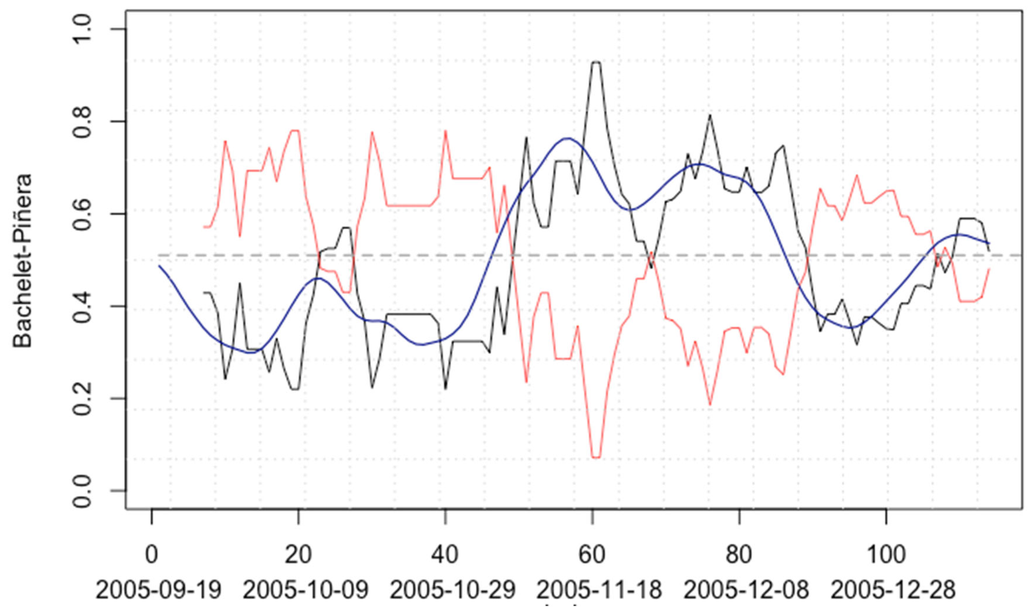
The results described below are favorable to the use of this data analysis technique. Each election is reviewed in detail, and the models that best fit the final result are compared. In the first modelling (

Table 2. Forecasting the results of the election between Michelle Bachelet and Sebastián Piñera 2006.

Variables	Time Series	ARIMA	Sigma ARIMA Model	p-Value Box Test by Ljung-Box	Average Forecasting Result	Election Result	Difference between Forecast and Election Result	Standard Error
Bachelet-Piñera 2006 (Relative)	Normal	(0,1,1)	0. 1632037	0.5138308	0.5084575	0.535	0.02761574	0.405063
	Moving Average	(2,1,3)	0.004500995	0.9093858	0.5389227	0.535	0.003642637	0.1053066
	Hodrick-Prescott	(2,1,2)	4.7742 × 10−6	0.9439797	0.527154	0.535	0.007846023	0.01271612

), we work with the 2006 presidential campaign between Michelle Bachelet and Sebastián Piñera. Three ARIMA models were applied: (0,1,1), (2,1,3), and (2,1,2), with sigma2 values suitable for the modelling process. One of the differences between the three models applied can be seen in the standard error which is highly variable. However, the ARIMA modelling for the Hodrick–Prescott smoothed series, which has a very low standard error, gave an excellent forecast, differing by only 0.78% from the final election result of 53.5% for Michelle Bachelet. On the other hand, the moving average forecast had an error of only 0.36% in relation to the final election result, but with a standard error of 10.53%, so the most reliable and effective modelling series, in this case, was Hodrick–Prescott, as presented in Figure 1.

In the second modelling (

Table 3. Forecasting the results of the 2010 election between Sebastián Piñera and Eduardo Frei.

Variables	Time Series	ARIMA	Sigma ARIMA Model	p-Value Box Test by Ljung-Box	Average Forecasting Result	Election Result	Difference between Forecast and Election Result	Standard Error
Piñera-Frei 2010 (Relative)	Normal	(0,0,1)	0.04846787	0.9696941	0.5992357	0.515	0.08423567	0.223711
	Moving Average	(1,0,0)	0.002123367	0.19944	0.5682475	0.515	0.05324748	0.06432831
	Hodrick-Prescott	(4,1,0)	9.841 × 10−7	0.8237633	0.5140846	0.515	0.0009154432	0.006677285

), we work with the 2009–2010 presidential campaign between Sebastián Piñera and Eduardo Frei as presented in Figure 2. Three ARIMA models were applied: (0,0,1), (1,0,0), and (4,1,0), with sigma2 values suitable for the modelling process. One of the differences between the three models applied can be seen in the standard error, which is highly variable although not as divergent as in the previous case. However, the ARIMA modelling for the series smoothed by Hodrick–Prescott is again the one with a very low standard error and offers the best forecast, differing only by 0.092% from the final election result of 51.5% for Sebastián Piñera. On the other hand, the moving average forecast, in this case, had an error of 5.32% in relation to the final election result, but with a standard error of 6.43%, so the most reliable and effective modelling series in this case was Hodrick–Prescott. If in this case and the previous one the modelling had been done only by moving average, the standard error does not allow detection of the definitive winner, since the variance may fall below 50% of preferences on who won the election, which is problematic beyond the fact that in all the averages of the forecasts the winner is given as the one who finally won the election.

In the third modelling (

Table 4. Forecasting results of the 2013 election between Michelle Bachelet and Evelyn Matthei.

Variables	Time Series	ARIMA	Sigma ARIMA Model	p-Value Box Test by Ljung-Box	Average Forecasting Result	Election Result	Difference between Forecast and Election Result	Standard Error
Bachelet-Matthei 2013 (Relative)	Normal	(1,0,1)	0.0156638	0.864565	0.6395573	0.6217	0.01785731	0.1307915
	Moving Average	(2,1,0)	0.0006456679	0.9911486	0.6905575	0.6217	0.06885749	0.04694867
	Hodrick-Prescott	(3,1,0)	4.422 × 10−7	0.8184402	0.6113527	0.6217	0.01034734	0.004601662

), we work with the 2013 presidential campaign between Michelle Bachelet and Evelyn Matthei as shown in Figure 3. Three ARIMA models were applied: (1,0,1), (2,1,0), and (3,1,0), with sigma2 values suitable for the modelling process. In this case, the standard error is less variable than in the two previous cases. The ARIMA modelling for the Hodrick–Prescott smoothed series has the lowest standard error and offers the best forecast, differing by only 1.03% from the final election result of 62.17% for Bachelet. Unlike the previous case, in this modelling, the moving average is no more accurate than the series without transformation, which had an error of 1.78% with the final result. The confirmation remains that the best model for this type of forecast is for a series smoothed by Hodrick–Prescott, which also remains at a very low standard error.

In the fourth modelling (

Table 5. Forecasting results of the 2017 election between Sebastián Piñera and Alejandro Guillier.

Variables	Time Series	ARIMA	Sigma ARIMA Model	p-Value Box Test by Ljung-Box	Average Forecasting Result	Election Result	Difference between Forecast and Election Result	Standard Error
Piñera-Guillier 2017 (Relative)	Normal	(1,1,1)	0.01176181	0.7434989	0.6652471	0.5458	0.1194471	0.1121784
	Moving Average	(1,1,0)	0.0005553617	0.8413091	0.6335689	0.5458	0.08776888	0.04116279
	Hodrick-Prescott	(3,1,0)	3.32157 × 10−7	0.6613639	0.611959	0.5458	0.06615895	0.00387286

), we work with the 2017 presidential campaign between Sebastián Piñera and Alejandro Guillier as shown in Figure 4. Three ARIMA models were applied: (1,1,1), (1,1,0) and (4,1,0), with sigma2 values suitable for the modelling process. Of all the modelling, this is the least accurate; by contrast, the best model is Hodrick–Prescott, which differs from the final result by 6.61%, which was favorable to Sebastián Piñera. What is interesting is that despite not being accurate, the fourth modelling predicts the winner and overestimates his/her influence rather than modelling indicatively that Guillier would win. In other words, in this case, the model is not accurate in the percentage result but still indicates the winning option effectively.

Finally,

Table 6. Forecasting the results of the 2020 election between Gabriel Boric and José Antonio Kast.

Variables	Time Series	ARIMA	Sigma ARIMA Model	p-Value Box Test by Ljung-Box	Average Forecasting Result	Election Result	Difference between Forecast and Election Result	Standard Error
Boric-Kast 2021 (Relative)	Normal	(2,0,0)	0.01887498	0.8072142	0.4623903	0.5564	0.0940097	0.140894
	Moving Average	(1,0,0)	0.000893124	0.2021044	0.5102202	0.5564	0.04617981	0.04325613
	Hodrick-Prescott	(2,2,3)	5.784 × 10−7	0.9772097	0.5612801	0.5564	0.004880149	0.004917933

indicates the outcome of the 2021 presidential election between Gabriel Boric and José Antonio Kast as shown in Figure 5. This modelling is the only one that presents a forecast that did not point to the definitive winner of the election, since the series without transformation gave Kast as the winner whereas Boric actually won. However, the Hodrick–Prescott modelling presents a forecast that only differs from the actual result by 0.48%, with a standard error of 0.49%.

4. Discussion

After applying the modelling to generate forecasts, it can be argued that the use of Google Trends to identify the candidates most likely to win in Chile is highly effective. The following table allows us to evaluate in summary the total of the forecasts developed. Undoubtedly, the most effective and accurate mechanism is that of smoothing with the Hodrick–Prescott technique, averaging a difference with the final result of 1.8% (

Table 7. Assessing the result of forecasts by election and ARIMA model used.

Election	Model	Assertion on Winner
Bachelet-Piñera 2006	Normal ARIMA: (0,1,1)	Yes
Bachelet-Piñera 2006	Moving Average ARIMA: (2,1,3)	Yes
Bachelet-Piñera 2006	Hodrick-Prescott ARIMA: (2,1,2)	Yes
Piñera-Frei 2010	Normal ARIMA: (0,0,1)	Yes
Piñera-Frei 2010	Moving Average ARIMA: (1,0,0)	Yes
Piñera-Frei 2010	Hodrick-Prescott ARIMA: (4,1,0)	Yes
Bachelet-Matthei 2013	Normal ARIMA: (1,0,1)	Yes
Bachelet-Matthei 2013	Moving Average ARIMA: (2,1,0)	Yes
Bachelet-Matthei 2013	Hodrick-Prescott ARIMA: (3,1,0)	Yes
Piñera-Guillier 2017	Normal ARIMA: (1,1,1)	Yes
Piñera-Guillier 2017	Moving Average ARIMA: (1,1,0)	Yes
Piñera-Guillier 2017	Hodrick-Prescott ARIMA: (3,1,0)	Yes
Boric-Kast 2021	Normal ARIMA: (2,0,0)	No
Boric-Kast 2021	Moving Average ARIMA: (1,0,0)	Yes
Boric-Kast 2021	Hodrick-Prescott ARIMA: (2,2,3)	Yes
Asserted?	NO	7%
	YES	93%
Difference with results	Average Normal Serie	6.86%
	Average Moving Average	5.19%
	Average Hodrick Prescott	1.80%

), a result inflated by the error in the case of the election between Sebastián Piñera and Alejandro Guillier in 2017. This indicates that to achieve greater precision, specific filtering mechanisms can be sought, filtering mechanisms that are temporally placed on what was being discussed on social media and what was being searched on Google during the election, in order to discern with greater understanding which keywords should be excluded from searches.

In the result analysis, out of the 15 models, only 1 model failed to identify the winner, i.e., for this analysis, 93% of the models do identify the winner of the election. Possibly, the application of other search cleaning strategies, associated with exclusionary keywords, could help to reduce the probability of error. However, the model is still effective when three techniques are applied simultaneously to assess which one might be providing information that confounds the interpretation of the forecasts. In any case, all the smoothed assessments, whether by moving average or Hodrick–Prescott, were successful in indicating who would win the election.

These results allow us to contribute to the international literature on the predictive electoral value of Google search trends. The assumption that could explain this predictive capacity is that people search for information on Google to inform their voting decision and in doing so allow us to record with good accuracy which of the electoral options is generating the most interest among the population. Google Trends also offers the possibility of exploring trends within each search in order to apply both filters and also to identify the topics associated with the searches that people are most interested in.

5. Conclusions

In Chile, Google penetration is significant, so the question arises as to whether this forecasting strategy would apply to other nations where there is less internet access or, conversely, whether in a nation with much greater internet access the model would gain or lose the predictive capability it shows in the modelling shown here. There is also the question of the ability to scale this type of search while maintaining good predictive results. In Chile, Google Trends allows the interest aroused by the words searched to be separated by region, so that a specific study can be carried out for each territory. In this case, no such test has been carried out. A very good predictive capacity has been proven, and one of the pending tasks is to move from a national analysis to specific regions or cities.

This study hypothesized that Google Trends generates valuable information about people’s preferences and that search trends can be used to generate effective forecasts on presidential elections. In the cases studied, the hypothesis was fulfilled and accepted as an effective method based on the following apparent constraints: voluntary voting or registration, two voting options, and the context of nationwide voting in Chile. Google Trends offers different fields of analysis that can be sorted in the form of time series. This opens up possibilities of exploring other aspects with similar techniques, such as trend variations in terms of most frequently used words, search priorities on a territory level, and even specific trends in urban locations such as cities or towns, when the search volume is recorded by Google.

The exercise of testing the predictive effectiveness of Google Trends for presidential elections in Chile has two factors that are relevant to consider for similar possible future studies: most of these elections are conducted with either voluntary voting or voluntary registration (as in Bachelet vs. Piñera 2006). The method has not been applied for elections with automatic registration, universal compulsory voting, or other types of elections other than presidential runoff elections. This is a limitation of the method used in this study and variations in results and the model’s own effectiveness. It is also important to investigate if this analysis technique is effective for similar contexts in other Latin American countries.