
Machine-Learning-Based Prediction of Corrosion Behavior in Additively Manufactured Inconel 718

Abstract
:
1. Summary
2. Data Description
2.1. Model Building
Database
2.2. Feature Selection
2.3. Model Development
2.3.1. Polynomial Regression
2.3.2. Support Vector Regression
2.3.3. Decision Tree
2.3.4. Extreme Gradient Boosting
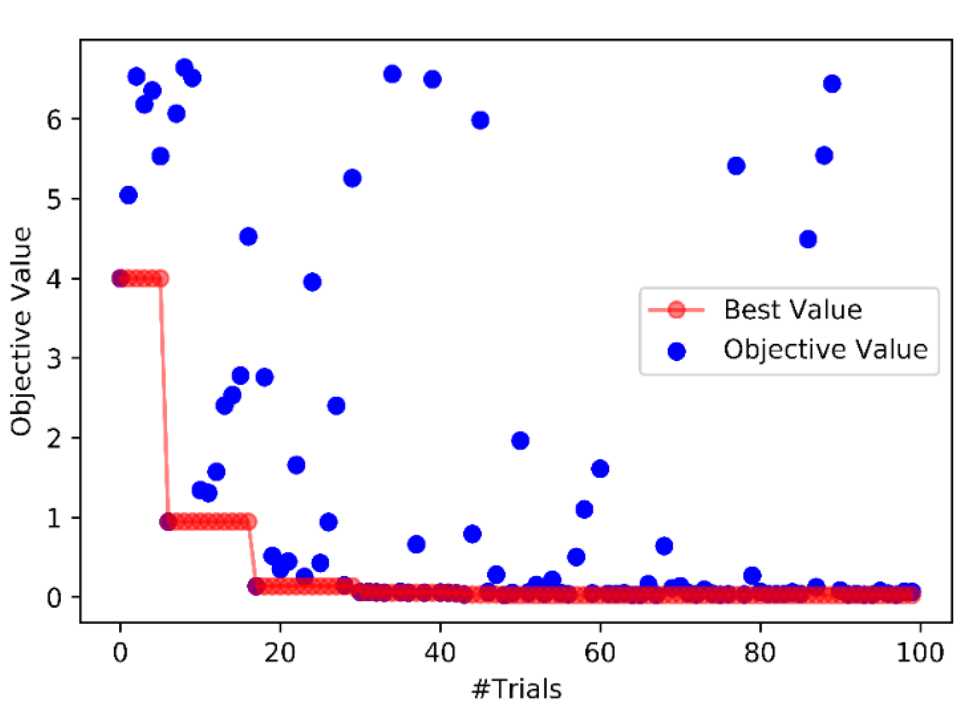
2.4. Hyperparameter Optimization
3. Methods
3.1. Model Validation
3.2. Feature Importance Analysis
4. Conclusions
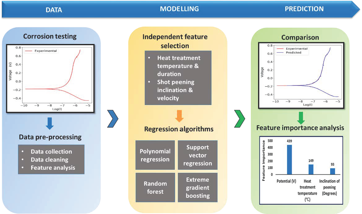
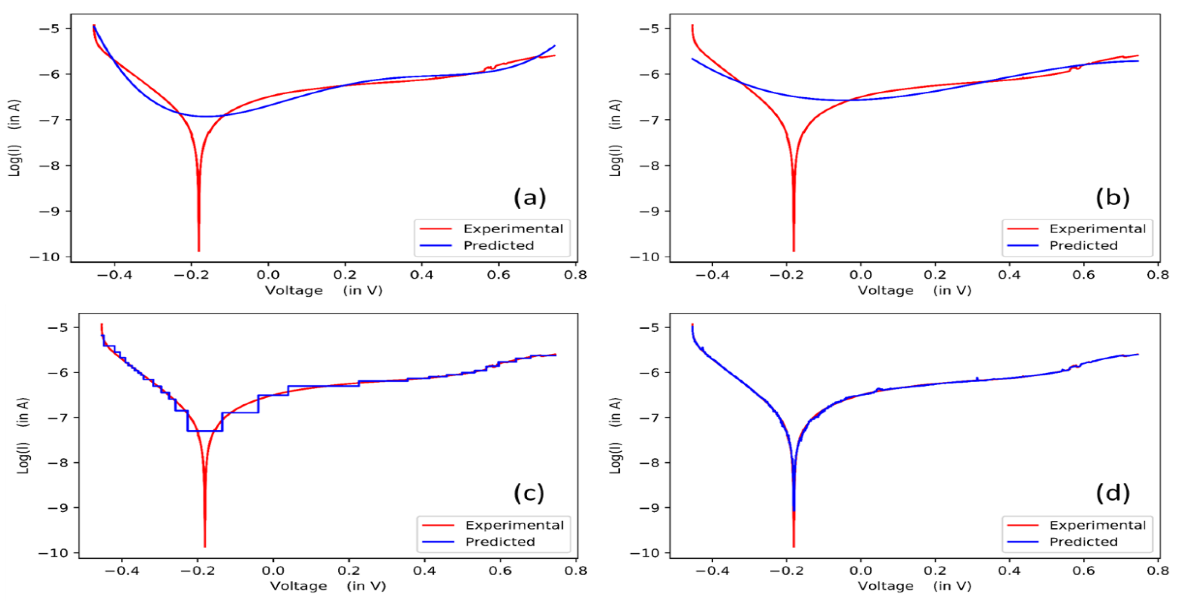
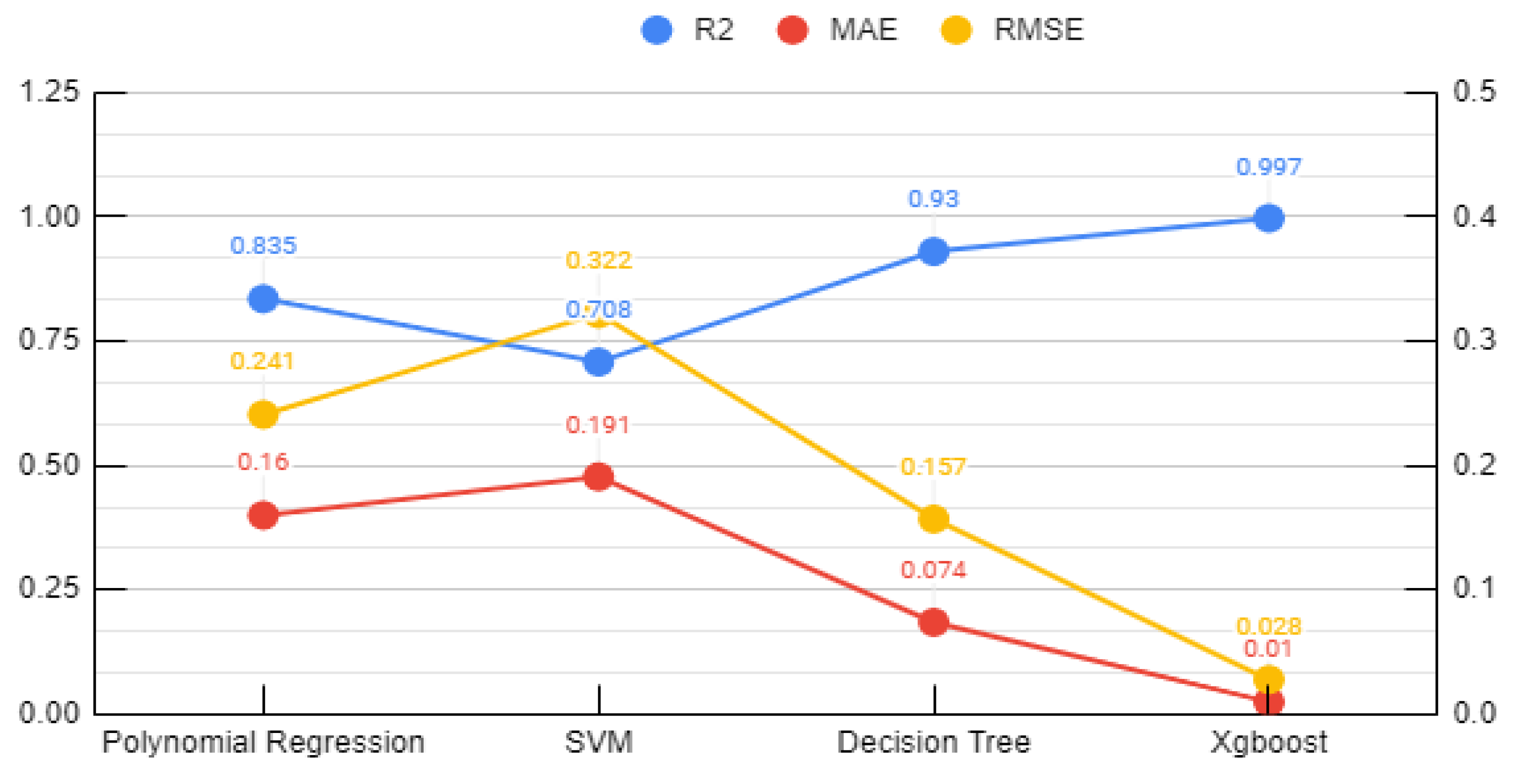
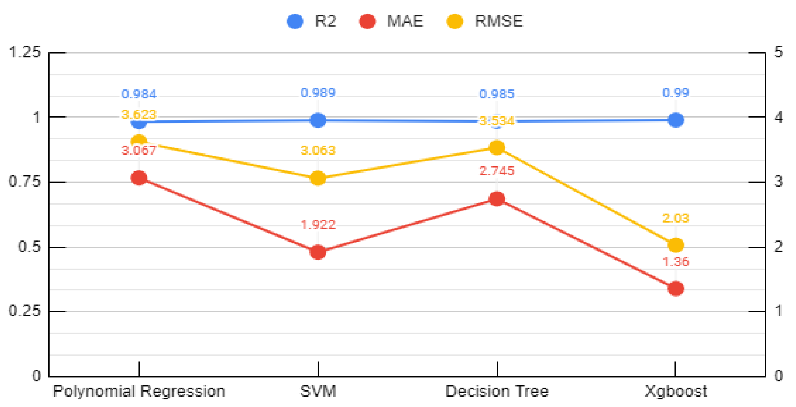
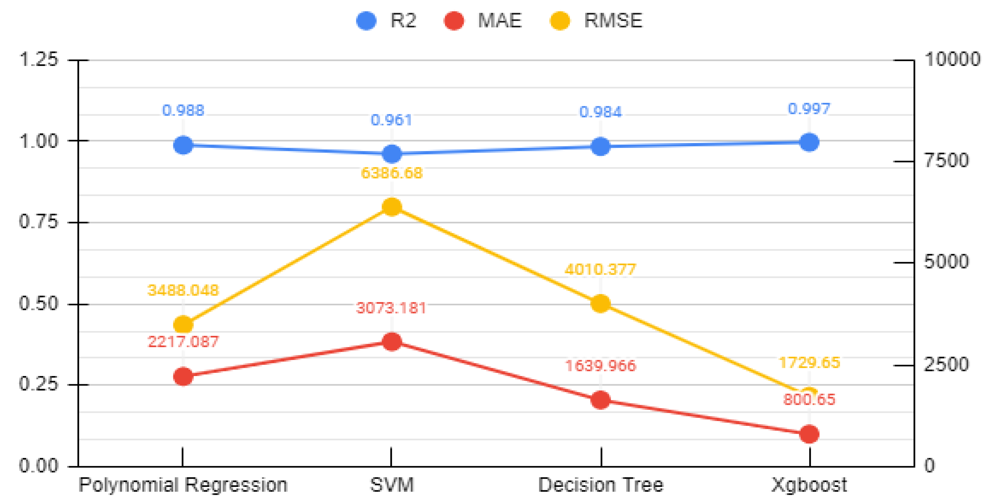
- Based on experimental data, the relationship between postprocessing techniques and corrosion resistance was explored using a machine learning approach. The feasibility of such an approach was demonstrated using four different ML algorithm namely, Polynomial regression, Support vector regression, Random forest and Extreme gradient boosting.
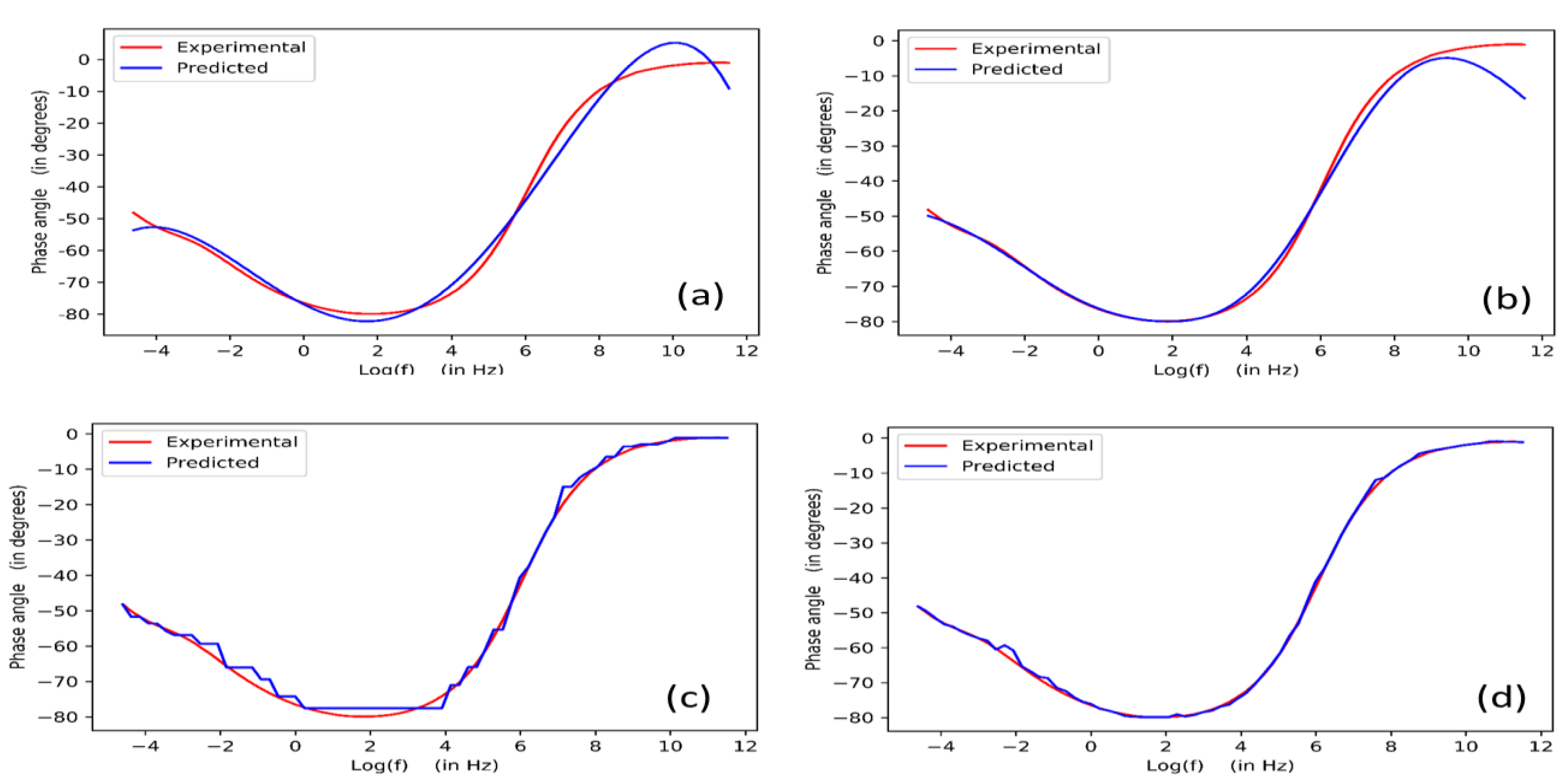
- In the development of ML-based models, the XGB algorithm led to the corrosion rate prediction of the alloy with the highest accuracy at an R2 value of 0.954 in PD testing and 0.997 in EIS testing.
- In the feature importance analysis, apart from the electrical parameters, heat treatment temperature and shot peening inclination were found to be the most influential parameters in determining the corrosion resistance of Inconel 718.
Author Contributions
Funding
Institutional Review Board Statement
Data Availability Statement
Conflicts of Interest
References
- Davis, J.R. ASM specialty handbook: Nickel, cobalt, and their alloys. Choice Rev. Online 2001, 38, 38–6206. [Google Scholar] [CrossRef]
- Pint, B.; Unocic, K.; Dryepondt, S. Oxidation of Superalloys in Extreme Environments. In Proceedings of the 7th International Symposium on Superalloy 718 and Derivatives (2010), Pittsburgh, PA, USA, 10–12 October 2010; pp. 861–875. [Google Scholar]
- Park, M. ASM Handbook Corrosion: Materials; American society of materials: Almere, The Netherlands, 2005. [Google Scholar]
- Akca, E.; Gürsel, A. A Review on Superalloys and IN718 Nickel-Based INCONEL Superalloy. Period. Eng. Nat. Sci. (PEN) 2017, 3. [Google Scholar] [CrossRef]
- Thomas, A.; El-Wahabi, M.; Cabrera, J.M.; Prado, J. High temperature deformation of Inconel 718. J. Mater. Process. Technol. 2006, 177, 469–472. [Google Scholar] [CrossRef]
- Mishra, A. Performance of Corrosion-Resistant Alloys in Concentrated Acids. Acta Met. Sin. Engl. Lett. 2017, 30, 306–318. [Google Scholar] [CrossRef] [Green Version]
- Soc, S.G.J.E. Corrosion of Steels and Nickel Alloys in Superheated Steam Corrosion of Steels and Nickel Alloys in Superheated Steam. J. Electrochem. Soc. 1964, 111, 1116. [Google Scholar]
- Delabrouille, F.; Legras, L.; Vaillant, F.; Scott, P.; Viguier, B.; Andrieu, E. Effect of the Chromium Content and Strain on the Corrosion of Nickel Based Alloys in Primary Water of Pressurized Water. In Proceedings of the 12th International Conference on Environmental Degradation of Materials in Nuclear Power System–Water Reactors, Salt Lake City, UT, USA, 14–18 August 2005. [Google Scholar]
- Mishra, A.K.; Shoesmith, D.W. Effect of Alloying Elements on Crevice Corrosion Inhibition of Nickel-Chromium-Molybdenum-Tungsten Alloys Under Aggressive Conditions: An Electrochemical Study. Corrosion 2014, 70, 721–730. [Google Scholar] [CrossRef]
- Cwalina, K.L.; Demarest, C.; Gerard, A.; Scully, J. Revisiting the effects of molybdenum and tungsten alloying on corrosion behavior of nickel-chromium alloys in aqueous corrosion. Curr. Opin. Solid State Mater. Sci. 2019, 23, 129–141. [Google Scholar] [CrossRef]
- Amigo, F.J.; Urbikain, G.; Pereira, O.; Fernández-Lucio, P.; Fernández-Valdivielso, A.; de Lacalle, L.L. Combination of high feed turning with cryogenic cooling on Haynes 263 and Inconel 718 superalloys. J. Manuf. Process. 2020, 58, 208–222. [Google Scholar] [CrossRef]
- Choi, J.-P.; Shin, G.-H.; Yang, S.; Yang, D.-Y.; Lee, J.-S.; Brochu, M.; Yu, J.-H. Densification and microstructural investigation of Inconel 718 parts fabricated by selective laser melting. Powder Technol. 2017, 310, 60–66. [Google Scholar] [CrossRef]
- Du, D.; Dong, A.; Shu, D.; Zhu, G.; Sun, B.; Li, X.; Lavernia, E. Influence of build orientation on microstructure, mechanical and corrosion behavior of Inconel 718 processed by selective laser melting. Mater. Sci. Eng. A 2019, 760, 469–480. [Google Scholar] [CrossRef]
- Baicheng, Z.; Xiaohua, L.; Jiaming, B.; Junfeng, G.; Pan, W.; Chen-Nan, S.; Muiling, N.; Guojun, Q.; Jun, W. Study of selective laser melting (SLM) Inconel 718 part surface improvement by electrochemical polishing. Mater. Des. 2017, 116, 531–537. [Google Scholar] [CrossRef]
- Li, H.; Feng, S.; Li, J.; Gong, J. Effect of heat treatment on the δ phase distribution and corrosion resistance of selective laser melting manufactured Inconel 718 superalloy. Mater. Corros. 2018, 69, 1350–1354. [Google Scholar] [CrossRef]
- Luo, S.; Huang, W.; Yang, H.; Yang, J.; Wang, Z.; Zeng, X. Microstructural evolution and corrosion behaviors of Inconel 718 alloy produced by selective laser melting following different heat treatments. Addit. Manuf. 2019, 30, 100875. [Google Scholar] [CrossRef]
- Calleja-Ochoa, A.; Gonzalez-Barrio, H.; de Lacalle, N.L.; Martínez, S.; Albizuri, J.; Lamikiz, A. A New Approach in the Design of Microstructured Ultralight Components to Achieve Maximum Functional Performance. Materials 2021, 14, 1588. [Google Scholar] [CrossRef]
- Almangour, B. Additive manufacturing of emerging materials. Addit. Manuf. Emerg. Mater. 2018, 1–355. [Google Scholar] [CrossRef]
- Debroy, T.; Wei, H.L.; Zuback, J.S.; Mukherjee, T.; Elmer, J.W.; Milewski, J.O.; Beese, A.M.; Wilson-Heid, A.D.; De, A.; Zhang, W. Additive manufacturing of metallic components–Process, structure and properties. Prog. Mater. Sci. 2018, 92, 112–224. [Google Scholar] [CrossRef]
- Kumar, S.; Pityana, S. Laser-Based Additive Manufacturing of Metals. Adv. Mater. Res. 2011, 227, 92–95. [Google Scholar] [CrossRef]
- Yap, C.Y.; Chua, C.K.; Dong, Z.; Liu, Z.H.; Zhang, D.Q.; Loh, L.E.; Sing, S.L. Review of selective laser melting: Materials and applications. Appl. Phys. Rev. 2015, 2, 041101. [Google Scholar] [CrossRef]
- Kaynak, Y.; Tascioglu, E. Post-processing effects on the surface characteristics of Inconel 718 alloy fabricated by selective laser melting additive manufacturing. Prog. Addit. Manuf. 2020, 5, 221–234. [Google Scholar] [CrossRef]
- Raghavan, S.; Zhang, B.; Wang, P.; Sun, C.-N.; Nai, M.L.S.; Li, T.; Wei, J. Effect of different heat treatments on the microstructure and mechanical properties in selective laser melted INCONEL 718 alloy. Mater. Manuf. Process. 2017, 32, 1588–1595. [Google Scholar] [CrossRef]
- Chen, L.; Sun, Y.; Li, L.; Ren, X. Microstructural evolution and mechanical properties of selective laser melted a nickel-based superalloy after post treatment. Mater. Sci. Eng. A 2020, 792, 139649. [Google Scholar] [CrossRef]
- Zhao, Y.; Guo, Q.; Ma, Z.; Yu, L. Comparative study on the microstructure evolution of selective laser melted and wrought IN718 superalloy during subsequent heat treatment process and its effect on mechanical properties. Mater. Sci. Eng. A 2020, 791, 139735. [Google Scholar] [CrossRef]
- Kermani, M.; Harrop, D. The Impact of Corrosion on Oil and Gas Industry. SPE Prod. Facil. 1996, 11, 186–190. [Google Scholar] [CrossRef] [Green Version]
- Finšgar, M.; Jackson, J. Application of corrosion inhibitors for steels in acidic media for the oil and gas industry: A review. Corros. Sci. 2014, 86, 17–41. [Google Scholar] [CrossRef] [Green Version]
- Tiu, B.D.; Advincula, R.C. Polymeric corrosion inhibitors for the oil and gas industry: Design principles and mechanism. React. Funct. Polym. 2015, 95, 25–45. [Google Scholar] [CrossRef]
- Groysman, A. Corrosion for Everybody; Springer: Berlin/Heidelberg, Germany, 2010; pp. 189–190. [Google Scholar] [CrossRef]
- Meade, C.L. Accelerated corrosion testing. Metal Finish. 2000, 98, 540–545. [Google Scholar] [CrossRef]
- Lorenz, W.J. Determination of corrosion rates by electrochemical DC and AC methods. Corros. Sci. 1981, 21, 647–672. [Google Scholar] [CrossRef]
- Mansfeld, S.F.; Tsai, I. Weight Studies of Atmospheric Corrosion—Loss and Electrochemical Measurements. Corros. Sci. 1980, 20, 1–3. [Google Scholar] [CrossRef]
- Sjding, A.B.J. Corrosion testing by potentiodynamic polarization in various electrolytes. Corros. Sci. 1992, 241–245. [Google Scholar]
- Mansfeld, F. Tafel slopes and corrosion rates obtained in the pre-Tafel region of polarization curves. Corros. Sci. 2005, 47, 3178–3186. [Google Scholar] [CrossRef]
- McCafferty, E. Validation of corrosion rates measured by the Tafel extrapolation method. Corros. Sci. 2005, 47, 3202–3215. [Google Scholar] [CrossRef]
- Chang, B.-Y.; Park, S.-M. Electrochemical Impedance Spectroscopy. Annu. Rev. Anal. Chem. 2006, 3, 207–229. [Google Scholar] [CrossRef]
- Agarwal, P.; Orazem, M.E.; Garcia-Rubio, L.H. Measurement models for electrochemical impedance spectroscopy: I. Demonstration of applicability. J. Electrochem. Soc. 1992, 139, 1917. [Google Scholar] [CrossRef]
- Park, S. With impedance data, a complete description of an electrochemical system is possible. Anal. Chem. 2003, 75, 455–461. [Google Scholar]
- Yu, X. Machine learning application in the life time of materials. arXiv 2017, arXiv:1707.04826. [Google Scholar]
- Irani, M.; Chalaturnyk, R.; Hajiloo, M. Application of data mining techniques in building predictive models for oil and gas problems: A case study on casing corrosion prediction. Int. J. Oil Gas Coal Technol. 2014, 8, 369–398. [Google Scholar] [CrossRef]
- Liu, Y.; Zhao, T.; Ju, W.; Shi, S. Materials discovery and design using machine learning. J. Mater. 2017, 3, 159–177. [Google Scholar] [CrossRef]
- Butler, K.T.; Davies, D.W.; Cartwright, H.; Isayev, O.; Walsh, A. Machine learning for molecular and materials science. Nat. Cell Biol. 2018, 559, 547–555. [Google Scholar] [CrossRef]
- Roh, Y.; Heo, G.; Whang, S.E. A Survey on Data Collection for Machine Learning. IEEE Trans. Knowl. Data Eng. 2019, 4347, 1–20. [Google Scholar] [CrossRef] [Green Version]
- Schmidt, J.; Marques, M.R.G.; Botti, S.; Marques, M.A.L. Recent advances and applications of machine learning in solid-state materials science. NPJ Comput. Mater. 2019, 5. [Google Scholar] [CrossRef]
- Yang, Q.; Liu, Y.; Chen, T.; Tong, Y. Federated Machine Learning: Concept and Applications. ACM Trans. Intell. Syst. Technol. 2019, 10, 1–19. [Google Scholar] [CrossRef]
- Sutton, C.; Boley, M.; Ghiringhelli, L.M.; Rupp, M.; Vreeken, J.; Scheffler, M. Identifying domains of applicability of machine learning models for materials science. Nat. Commun. 2020, 11, 1–9. [Google Scholar] [CrossRef] [PubMed]
- Kailkhura, B.; Gallagher, B.; Kim, S.; Hiszpanski, A.; Han, T.Y.-J. Reliable and explainable machine-learning methods for accelerated material discovery. NPJ Comput. Mater. 2019, 5, 1–9. [Google Scholar] [CrossRef]
- Wen, Y.; Cai, C.; Liu, X.; Pei, J.; Zhu, X.; Xiao, T. Corrosion rate prediction of 3C steel under different seawater environment by using support vector regression. Corros. Sci. 2009, 51, 349–355. [Google Scholar] [CrossRef]
- Kamrunnahar, M.; Urquidi-Macdonald, M. Prediction of corrosion behavior using neural network as a data mining tool. Corros. Sci. 2010, 52, 669–677. [Google Scholar] [CrossRef]
- Gong, X.; Dong, C.; Xu, J.; Wang, L.; Li, X. Machine learning assistance for electrochemical curve simulation of corrosion and its application. Mater. Corros. 2019, 71, 474–484. [Google Scholar] [CrossRef]
- Zhu, S.; Sun, X.; Gao, X.; Wang, J.; Zhao, N.; Sha, J. Equivalent circuit model recognition of electrochemical impedance spectroscopy via machine learning. J. Electroanal. Chem. 2019, 855, 113627. [Google Scholar] [CrossRef] [Green Version]
- Watson, J.; Taminger, K. A decision-support model for selecting additive manufacturing versus subtractive manufacturing based on energy consumption. J. Clean. Prod. 2018, 176, 1316–1322. [Google Scholar] [CrossRef]
- Mythreyi, O.V.; Raja, A.; Nagesha, B.K.; Jayaganthan, R. Corrosion Study of Selective Laser Melted IN718 Alloy upon Post Heat Treatment and Shot Peening. Metals 2020, 10, 1562. [Google Scholar] [CrossRef]
- Cai, J.; Luo, J.; Wang, S.; Yang, S. Feature selection in machine learning: A new perspective. Neurocomputing 2018, 300, 70–79. [Google Scholar] [CrossRef]
- Vafaie, H.; De Jong, K. Genetic Algorithms as a Tool for Feature Selection in Machine Learning. In Proceedings of the IEEE International Conference on Tools with Artificial Intelligence, Arlington, VA, USA, 10–11 November 1992. [Google Scholar]
- Ostertagová, E. Modelling using Polynomial Regression. Procedia Eng. 2012, 48, 500–506. [Google Scholar] [CrossRef] [Green Version]
- Smola, A.J.; Schölkopf, B. A tutorial on support vector regression. Stat. Comput. 2004, 14, 199–222. [Google Scholar] [CrossRef] [Green Version]
- Czajkowski, M.; Kretowski, M. The role of decision tree representation in regression problems—An evolutionary perspective. Appl. Soft Comput. 2016, 48, 458–475. [Google Scholar] [CrossRef]
- Guttenberg, N. Learning to generate classifiers. arXiv 2018, arXiv:1803.11373. [Google Scholar]
- Zemel, R.S. A Gradient-Based Boosting Algorithm for Regression Problems. In Proceedings of the 13th International Conference on Neural Information Processing Systems, Hong Kong, China, 3–6 October 2006. [Google Scholar]
- Chen, T. XGBoost: A Scalable Tree Boosting System. In Proceedings of the 22nd Acm Sigkdd International Conference on Knowledge Discovery and Data Mining, San Francisco, CA, USA, 13–17 August 2016. [Google Scholar]
- You, X.; Tan, Y.; Zhao, L.; You, Q.; Wang, Y.; Ye, F.; Li, J. Effect of solution heat treatment on microstructure and electrochemical behavior of electron beam smelted Inconel 718 superalloy. J. Alloys Compd. 2018, 741, 792–803. [Google Scholar] [CrossRef]
- Mylonas, G.; Labeas, G. Numerical modelling of shot peening process and corresponding products: Residual stress, surface roughness and cold work prediction. Surf. Coat. Technol. 2011, 205, 4480–4494. [Google Scholar] [CrossRef]
- Bagherifard, S.; Ghelichi, R.; Guagliano, M. Numerical and experimental analysis of surface roughness generated by shot peening. Appl. Surf. Sci. 2012, 258, 6831–6840. [Google Scholar] [CrossRef]
- Walter, R.; Kannan, M.B. Influence of surface roughness on the corrosion behaviour of magnesium alloy. Mater. Des. 2011, 32, 2350–2354. [Google Scholar] [CrossRef]
- Kovacı, H.; Bozkurt, Y.; Yetim, A.; Aslan, M.; Çelik, A. The effect of surface plastic deformation produced by shot peening on corrosion behavior of a low-alloy steel. Surf. Coat. Technol. 2019, 360, 78–86. [Google Scholar] [CrossRef]


| Specimen Conditions | AB, HT, SP, HTSP |
|---|---|
| Corrosion testing methods used | Potentiodynamic polarization, electrochemical impedance spectroscopy |
| Postprocessing used | Heat treatment, shot peening |
| Testing environment | 3.5 wt% NaCl environment |
| Mode of corrosion tested | Aqueous, general corrosion |
| Data source | Gamry 600+, electrochemical workstation software |
| Corrosion plots used | PD, Bode, Nyquist |
| Parameter | Value |
|---|---|
| Heat treatment temperature | 980 °C |
| Heat treatment duration | 15 min |
| Shot peening inclination | 45° |
| Shot peening velocity | 70 m/s |
| Independent Parameters for the Tafel Plot | |||||
|---|---|---|---|---|---|
| Sample Condition | Heat Treatment Temperature (°C) | Heat Treatment Duration (Min) | Shot Peening Velocity (m/s) | Shot Peening Inclination (Degrees) | Voltage (Volts) |
| AB | 0 | 0 | 0 | 0 | −4.77 × 10⁻¹ |
| HT | 980 | 15 | 0 | 0 | −4.74 × 10⁻¹ |
| SP | 0 | 0 | 70 | 45 | −4.27 × 10⁻¹ |
| HTSP | 980 | 15 | 70 | 45 | −4.71 × 10⁻¹ |
| Independent Parameters for the Bode Plot | |||||
|---|---|---|---|---|---|
| Sample Condition | Heat Treatment Temperature (°C) | Heat Treatment Duration (min) | Shot Peening Velocity (m/s) | Shot Peening Inclination (Degrees) | Frequency (Hz) |
| AB | 0 | 0 | 0 | 0 | 79,450 |
| HT | 980 | 15 | 0 | 0 | 63,140 |
| SP | 0 | 0 | 70 | 45 | 50,200 |
| HTSP | 980 | 15 | 70 | 45 | 39,890 |
| Independent Parameters for the Nyquist Plot | |||||
|---|---|---|---|---|---|
| Sample Condition | Heat Treatment Temperature (°C) | Heat Treatment Duration (min) | Shot Peening Velocity (m/s) | Shot Peening Inclination (Degrees) | Impedance {Real} (Ohm) |
| AB | 0 | 0 | 0 | 0 | 27.59 |
| HT | 980 | 15 | 0 | 0 | 31.05 |
| SP | 0 | 0 | 70 | 45 | 26.97 |
| HTSP | 980 | 15 | 70 | 45 | 27.42 |
| Algorithm | Parameters | Range |
|---|---|---|
| XGB | booster | [‘gbtree’, ‘gblinear’, ‘dart’] |
| reg_lambda | [1 × 10⁻⁴, 1.0] | |
| reg_alpha | [1 × 10⁻⁴, 1.0] | |
| n_estimators | [10, 100] | |
| learning_rate | [1 × 10⁻⁴, 1.0] | |
| max_depth | [1, 6] | |
| DT | splitter | [“best”, “random”] |
| criterion | [“mse”, ”mape”] | |
| Max_features | [“auto”, “sqrt”, “log2”] | |
| min_samples_leaf | [10, 1000] | |
| max_depth | [1, 6] | |
| SVR | kernel | [linear’, ‘poly’, ‘rbf’] |
| C | [1.0, 100.0] | |
| gamma | [‘scale’, ‘auto’] | |
| epsilon | [0.1, 1] | |
| PR | degree | [1–6] |
Publisher’s Note: MDPI stays neutral with regard to jurisdictional claims in published maps and institutional affiliations. |
© 2021 by the authors. Licensee MDPI, Basel, Switzerland. This article is an open access article distributed under the terms and conditions of the Creative Commons Attribution (CC BY) license (https://creativecommons.org/licenses/by/4.0/).
Share and Cite
Mythreyi, O.V.; Srinivaas, M.R.; Amit Kumar, T.; Jayaganthan, R. Machine-Learning-Based Prediction of Corrosion Behavior in Additively Manufactured Inconel 718. Data 2021, 6, 80. https://doi.org/10.3390/data6080080
Mythreyi OV, Srinivaas MR, Amit Kumar T, Jayaganthan R. Machine-Learning-Based Prediction of Corrosion Behavior in Additively Manufactured Inconel 718. Data. 2021; 6(8):80. https://doi.org/10.3390/data6080080
Chicago/Turabian StyleMythreyi, O. V., M. Rohith Srinivaas, Tigga Amit Kumar, and R. Jayaganthan. 2021. "Machine-Learning-Based Prediction of Corrosion Behavior in Additively Manufactured Inconel 718" Data 6, no. 8: 80. https://doi.org/10.3390/data6080080
APA StyleMythreyi, O. V., Srinivaas, M. R., Amit Kumar, T., & Jayaganthan, R. (2021). Machine-Learning-Based Prediction of Corrosion Behavior in Additively Manufactured Inconel 718. Data, 6(8), 80. https://doi.org/10.3390/data6080080