The Hierarchical Classifier for COVID-19 Resistance Evaluation

Abstract

Finding dependencies in the data requires the analysis of relations between dozens of parameters of the studied process and hundreds of possible sources of influence on this process. Dependencies are nondeterministic and therefore modeling requires the use of statistical methods for analyzing random processes. Part of the information is often hidden from observation or not monitored. That is why many difficulties have arisen in the process of analyzing the collected information. The paper aims to find frequent patterns and parameters affected by COVID-19. The novelty of the paper is hierarchical architecture comprises supervised and unsupervised methods. It allows the development of an ensemble of the methods based on k-means clustering and classification. The best classifiers from the ensemble are random forest with 500 trees and XGBoost. Classification for separated clusters gives us higher accuracy on 4% in comparison with dataset analysis. The proposed approach can be used also for personalized medicine decision support in other domains. The features selection allows us to analyze the following features with the highest impact on COVID-19: age, sex, blood group, had influenza.

1. Introduction

The trend of the disease in most countries of the world and Ukraine continues to deteriorate [1]. The nature of the increase in the number of sick people changed from linear in May–August 2020 to a clear exponential in September–October this year. During October–November, the situation threatens to become extremely difficult, especially for the country’s medical system.

The difficulty in analyzing and forecasting the spread of COVID-19 is the indisputable difference between real data and official statistics published by the National Health Service of Ukraine [2], the National Security and Defense Council of Ukraine, and other sources. The main reasons for this are the following:

• The number of tests in Ukraine is insufficient to identify a real picture of the spread of the disease [3], which doubt the adequacy of the data, especially at the beginning of the epidemic—during the first—quarantine period. For comparison, according to the WHO report dated 3rd September 2020, 1 million 621 thousand 697 tests were performed in Ukraine, which is 0.48 tests per 1000 population. In the United States, 2.19 tests were performed per 1000 population. In the UAE, testing reaches almost 8 tests per 1 thousand of population. In Germany, 1.68 tests were performed per 1000 population.
• Many people, recognizing well-known symptoms, do not rush to report it to their doctor, but are treated on their own, continuing to spread the disease, and, accordingly, with a successful recovery, do not get into the official statistics.
• The rate of increase or decrease in daily morbidity should primarily depend on the actual number of active patients. However, it is also necessary to take into account the insufficient amount of laboratory tests, which does not allow timely diagnosis, insufficient effectiveness of diagnostic methods, which also reduces the reliability of official data [4].

Even though intelligent machine learning algorithms [4], neural networks [5], and SARIMA-type models [6] used in research are able to determine certain “patterns” and trends in the behavior of the studied phenomena, it is impossible to obtain a high accuracy prediction under the above circumstances [5]. It can only indicate the defining trends and patterns of disease spread.

That is why the aim of the paper is to find frequent patterns and to find parameters affected by COVID-19. Our approach consists of a hierarchical classifier as comprising supervised and unsupervised methods.

The main contribution of this paper can be summarized as follows:

• − a dataset from three countries (Ukraine, Germany, and Belarus) was collected, which allowed a more in-depth analysis and generalization;
• − hypothesis that patients with blood group II are more vulnerable to COVID-19;
• − the features affected by COVID-19 cases were selected based on machine learning algorithms and comparison of their results;
• − the proposed hierarchical classifier based on the combined use of unsupervised and supervised machine learning algorithms provide higher accuracy on 4% in comparison with random forest and XGBoost algorithms.

Thus, the frequent pattern for COVID-19 resistance can be found. The proposed approach can be used also for personalized medicine decision support in other domains. The developed pattern of resistance patient to COVID-19 allows more accurate estimation of new cases based on traditional models such as SSIR, SEIR, SARIMA, etc.

The structure of the paper is following. Section 2 represents the literature review and approach for the spread of virus modeling. The dataset description is given in Section 3. Section 4 represents the estimation of quality metrics for the existing clustering method. Next, the novel approach based on an ensemble of the clustering and classification methods is developed. Section 5 reports the results of the proposed approach. The conclusion underlines the novelty of the proposed approach.

2. Literature Review

COVID-19 is known to be one of the influenza virus variants [6]. When ingested, specific antibodies (Ig) are produced that are intended to combat the virus and are major markers in the study that are capable of showing whether the virus is present in the body. Thus, predominantly the presence of viruses in the blood indicates the presence of specific IgG, and the sign of a transmitted viral infection is the presence in the body of IgM [7]. However, the appearance of these and other specific immunoglobulins may be associated with the transmission of a history of other types of viral infection, the preliminary vaccination against influenza, including tuberculosis.

The main idea is to analyze rapid tests and answers in the questionnaire: was/were vaccinated against influenza, tuberculosis, and whether they were ill with influenza/tuberculosis this year. Additionally, a person should indicate which blood group they have. Compared to other regions or countries, it will probably reveal the causes of different incidence of COVID-19 in different countries.

The main methods used to build a predictive model and calculate the spread of COVID-19 virus are the following:

• data mining [8];
• principle of similarity in mathematical modeling [9];
• correlation analysis [10];
• regression analysis [11].

Autoregressive integrated moving average, or ARIMA, is one of the most widely used forecasting methods for univariate forecasting of time series data [12]. Although the method can handle trending data, it does not support seasonal component time series [13]. The ARIMA extension that supports direct modeling of the seasonal component of the series is called SARIMA [14]. The problem with ARIMA is that it does not support seasonal data. This is a time series with a repeating cycle. ARIMA expects data that is not seasonal or has a seasonal component removed, for example, seasonally adjusted using techniques such as seasonal variance.

Seasonal autoregressive integrated moving average, SARIMA or seasonal ARIMA, is an extension of ARIMA that explicitly supports univariate time series data with a seasonal component [15]. It adds three new hyperparameters for specifying autoregressive (AR), difference (I), and moving average (MA) for the seasonal component of the series, as well as an additional parameter for the seasonality period. The seasonal ARIMA model is formed by including additional seasonal terms in ARIMA [16]. The seasonal portion of the model consists of terms that are very similar to the non-seasonal components of the model, but include reverse shifts of the seasonal period [17].

The special methods for virus modeling are analyzed in [18]. The biggest problem is the uncertainty of the available official data, especially regarding the real initial number of infected (cases), which can lead to ambiguous results and inaccurate forecasts for the order, which was also pointed out by other investigators.

That is why the agent approach is combined with the SEIR-model in [19]. The following agents are used: person, house, business, government, healthcare system. The COVID-ABS approach was capable to effectively simulate social intervention scenarios. However, it is impossible to find the source of spread of virus.

The task of finding dependencies in the data requires the analysis of dependencies between dozens of parameters of the studied process and hundreds of possible sources of influence on this process. Dependencies are nondeterministic and therefore modeling requires the use of statistical methods for analyzing random processes [20]. Part of the information is often hidden from observation or not monitored. That is why many difficulties have arisen in the process of analyzing the collected information.

Today, the developed methods of statistical analysis allow working with partially uncertain or vague processes. However, the available methods have significant limitations in the scope and data types.

The purpose of the paper is to find the dependence between individual parameters of separated responder (age, sex, blood group, etc.) and COVID-19 resistance. The frequent pattern of resistant people based on this dependence should be developed. The travel restriction, isolation, quarantine, lock down, and social distancing are not taken into account. That is why we do not use the SEIR model, which allows to predict the number of new cases.

Thus, all the above factors may adversely affect the conduct, interpretation, and generalization of research results and the understanding and interpretation of the phenomenon under study.

3. Dataset Description

The dataset [21] is collected using Google form (Appendix A), is funded by the Central European Initiative, and verified by Lviv regional center COVID’19 resistance. The project Stop COVID-19 [22] has use case, implemented in Ukraine and Belarus. Partners from Germany shared Google form too and helped in data collection. The dataset is collected data over the period from 1 September to 29 October. The dataset provides data of COVID-19 unconfirmed and confirmed cases [21].

This dataset consists of the following characteristics:

• Age (categorical): 1:<15, 2: 16–22, 3: 23–40, 4: 41–65, 5: >66;
• Sex (categorical): male, female;
• Region (string): Lviv (Ukraine), Chernivtsi (Ukraine), Belarus, Germany, Other;
• Do you smoke (Boolean): 2: yes, 0: no;
• Have you had COVID (categorical): 2: yes, 0: no, 1: maybe;
• IgM level (numerical): [0..0.9) (negative), [0.9..1.1) (indefinite), ≥1.1 (positive);
• IgG level (numerical): [0..0.9) (negative), [0.9..1.1) (indefinite), ≥1.1 (positive);
• Blood group (categorical): 1, 2, 3, 4;
• Do you vaccinate for influenza? (categorical): 2: yes, 0: no, 1: maybe;
• Do you vaccinate for tuberculosis? (categorical): 2: yes, 0: no, 1: maybe;
• Have you had influenza this year? (categorical): 2: yes, 0: no, 1: maybe;
• Have you had tuberculosis this year? (categorical): 2: yes, 0: no, 1: maybe.

Characteristics IgG and IgM represent the result of rapid tests and anti-SARS-CoV-2 IgG and IgM kits. The number of IgG and IgM antibodies is different for different times after infection. That is why not only categorical meaning (positive, indefinite, or negative), but also exact values of these attributes are taken into account.

A total of 313 responses are presented in the dataset. Thirty-eight rows have empty values.

4. Materials and Methods

In predictive analytics machine learning methods, in particular, neural networks, are often mentioned [23]. However, in this case, the effectiveness of their use will be small. The main reason is that machine learning models are worthwhile in the case of stationary processes. It is assumed that future forecasting data are described by the same distribution as the training data. However, the growth of detected cases of coronavirus is a significantly non-stationary process. In addition, to identify complex patterns by machine learning methods, it is necessary to have large enough training samples with a sufficient number of informative features, such as patient conditions, behavior in different regions, attendance at different institutions, and so on. Currently, such features are analyzed by various specialists and when such data are widely available, machine learning methods will be able to show their effectiveness [3,4,8].

In our point of view, models that combine available data and expert opinion are effective. These can be parametric models, i.e., models that describe the process of coronavirus spread using some formula with parameters. The values of these parameters should describe the available data by the selected model. In the simple case, if the time derivative of the number of coronavirus cases is proportional to the total number of cases, then the solution of such diffraction is described by an exponential function. In logarithmic scale, we obtain a linear dependence, the parameters of which can be found by the method of least squares. However, the exponential nature of the number of detected cases can describe the process only for a certain period of time, the number of cases is limited by the number of people who can potentially catch the virus. Thus, after some time, the pandemic should end, and the number of cases should reach saturation. This process can be modeled using a logistic curve.

It is also important to assess the uncertainty of the forecast, the limits of changes in forecast values. One of the beneficial approaches, in our opinion, is the usage of Bayesian inference, which are based on Bayesian theorem [24]. The least squares method makes it possible to find constant coefficients for the models and, accordingly, some predicted value. With the help of Bayesian regression, it is possible to find distributions for model parameters and accordingly estimate the uncertainty of forecasting, which is important for a small amount of data.

Thus, the results of Bayesian inference prediction can be seen as a compromise between historical data and expert opinion, which is important for cases with small dataset. The logistics curve model can be useful when distribution has exponential growth of detected coronavirus cases.

Analysis of the spread of the COVID-19 epidemic in different countries shows the different nature of virus affection [25]. That is why our idea is to find parameters that affect the spread of the COVID-19 epidemic.

4.1. Data Preprocessing

First, the data preprocessing is provided. The main assumption of the analysis: all who filled out the form were either ill or had symptoms. The data distribution is analyzed.

RStudio is used for data analysis. By using packages factoextra, cluster, corrplot, and caret, the biggest part of the methods was implemented.

The instances selection is based on data distribution.

The distribution of dataset characteristics is given in

Table 1. Age, sex, region and COVID distribution.

#	Age	n
1	23–40	124
2	40–65	84
3	16–22	82
4	>65	19
5	<15	4
#	Sex	n
1	Male	178
2	Female	135
#	Region	n
1	Ukraine, Lviv	159
2	Ukraine, Chernivtsi	67
3	Belarus	56
4	Germany	27
5	others	4
#	COVID	n
1	yes	105
2	no	100
3	maybe	78

. Frequency of <15 age is lower than 0.013. That is why 4 rows are deleted. Sex distribution is relatively the same.

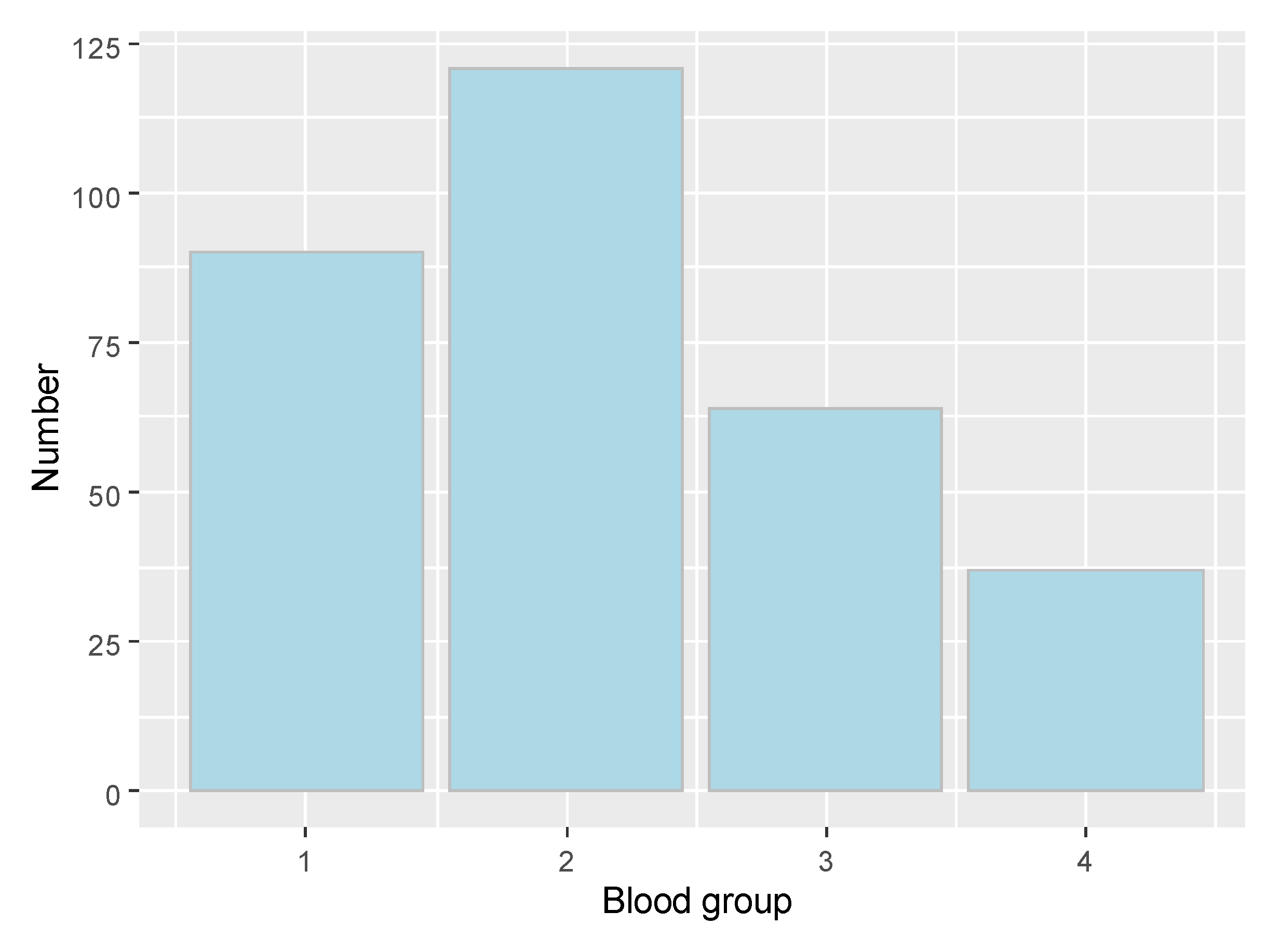
Distribution based on blood group is presented in Figure 1. Confirmed cases distribution by blood group is the following: 1 group—58, 2 group—76, 3 group—18, 4 group—15.

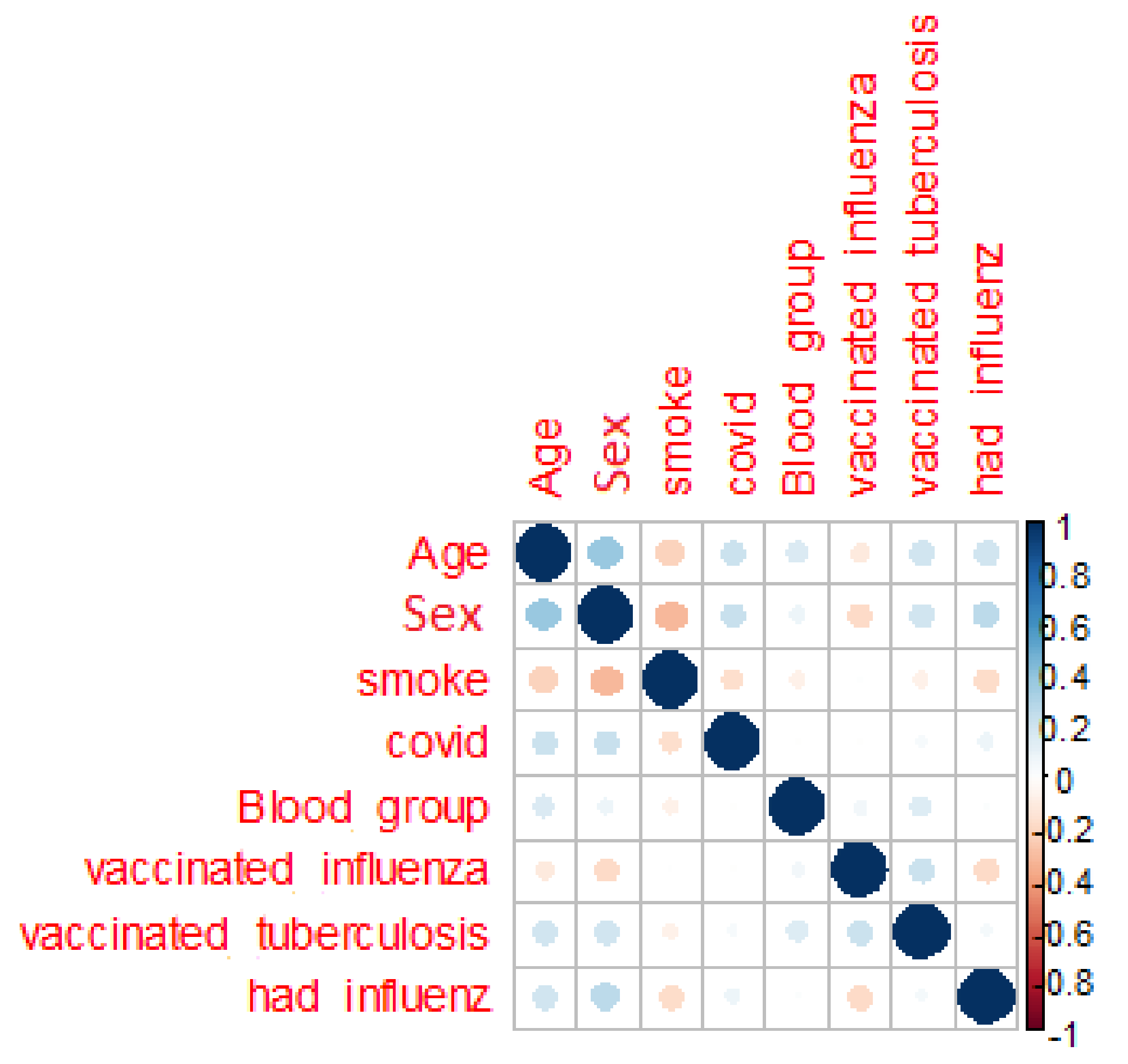
The next assumption is the correlation between features (Figure 2) for seeking persons and persons with unknown diagnose.

The presented correlation matrix shows lack of dependent parameters for the whole dataset. The target attribute COVID is clearly not defined by features.

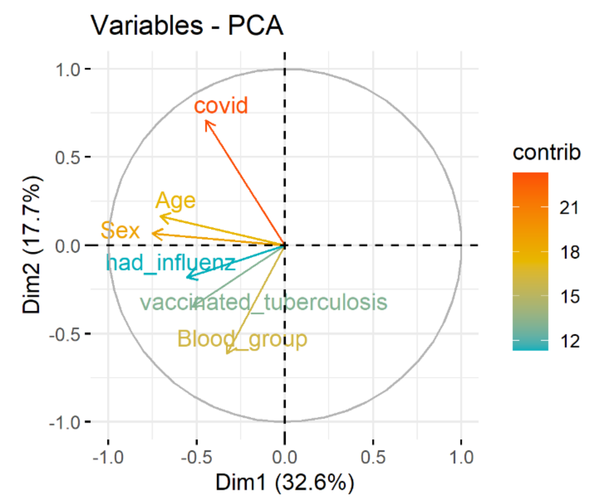
Spectral decomposition, which examines the covariance/correlation between variables, is developed using principle component analysis (PCA). The dependence between variables is given in Figure 3. Positively correlated variables point to the same side of the plot. Negatively correlated variables point to opposite sides of the graph. Therefore, the correlation between COVID and age, sex, blood group, vaccinated tuberculosis, had influenza is presented.

The next step is clustering and data analysis inside clusters.

4.2. Cluster Analysis

4.2.1. COVID-19 Dataset Clustering

Clustering methods require finding the distance between instances. That is why one-hot-encoding is used for categorical data transformation to numerical data for clustering.

First, we try to find clusters and use these clusters for future analysis. The first method is k-means algorithm with 4 clusters estimated by gaps-statistics [26]. Visualization of k-means shows intersection between clusters (Figure 4). This requires the future analysis.

The tendency of clustering is analyzed. Hopkins statistics (H) [27] shows that data distribution is not uniform. That means the data are good for clustering:

H = 0.5940309.

(1)

4.2.2. Analysis of Each Cluster

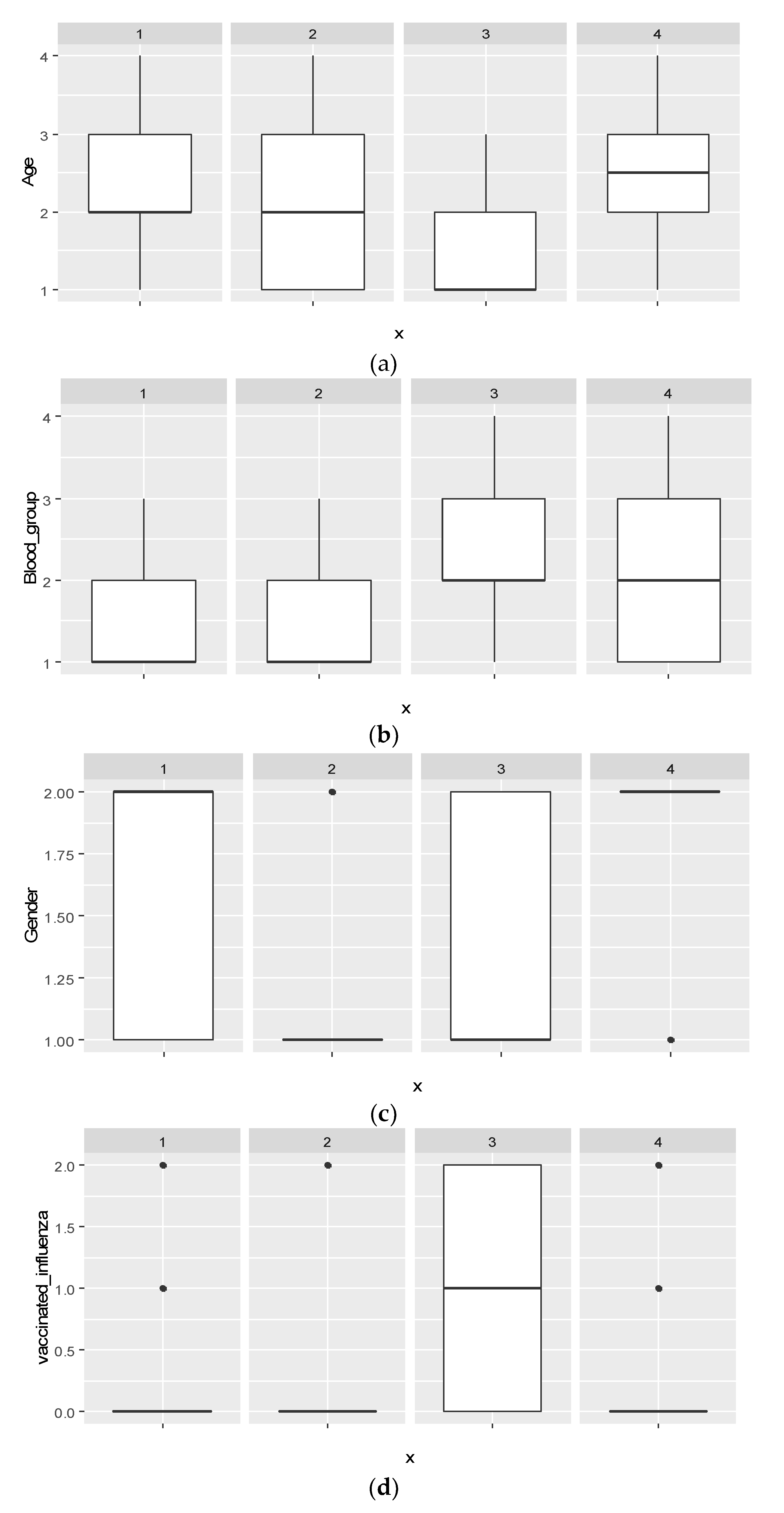
The next step is to analyze each cluster separately (Figure 5).

As you can see, the distributions in different clusters are completely different to each other: not only median values differ, but also the spread of values. However, it is worth mentioning that “box-and-whiskers diagrams” are most informative when the data distribution is normal or close to normal. Cluster 2 consists of only men, and cluster 4 consists of only women. Persons vaccinated against influenza are presented only in cluster 3.

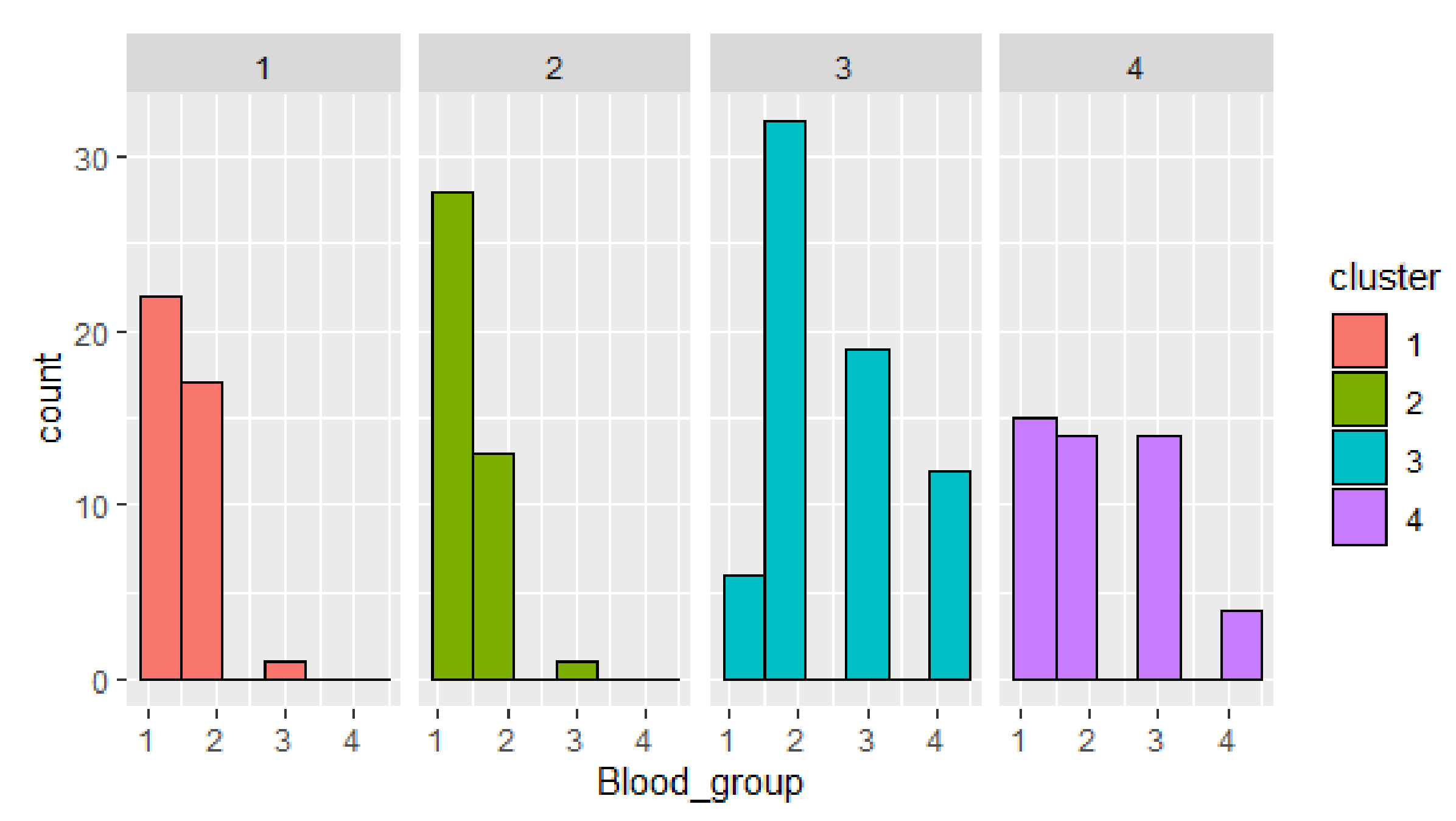
Next, cluster objects distribution by parameters is given (Figure 6). Cluster 3 has the biggest number of confirmed cases. The most frequent is blood group 2. This fact confirms the hypothesis that patients with blood group II are more vulnerable to COVID-19 for the mentioned dataset. The smallest number of confirmed cases is given in cluster 4.

The visualization of the clusters distribution by blood group shows outliers in clusters 1 and 2 (blood group 3), in cluster 3 (blood group 1), and uniform distribution of persons with blood group 1–3 in cluster 4.

4.3. Classification

We try to build the classifier for the whole dataset. The target variable will be “Have you had COVID”, the rest of variables will be features.

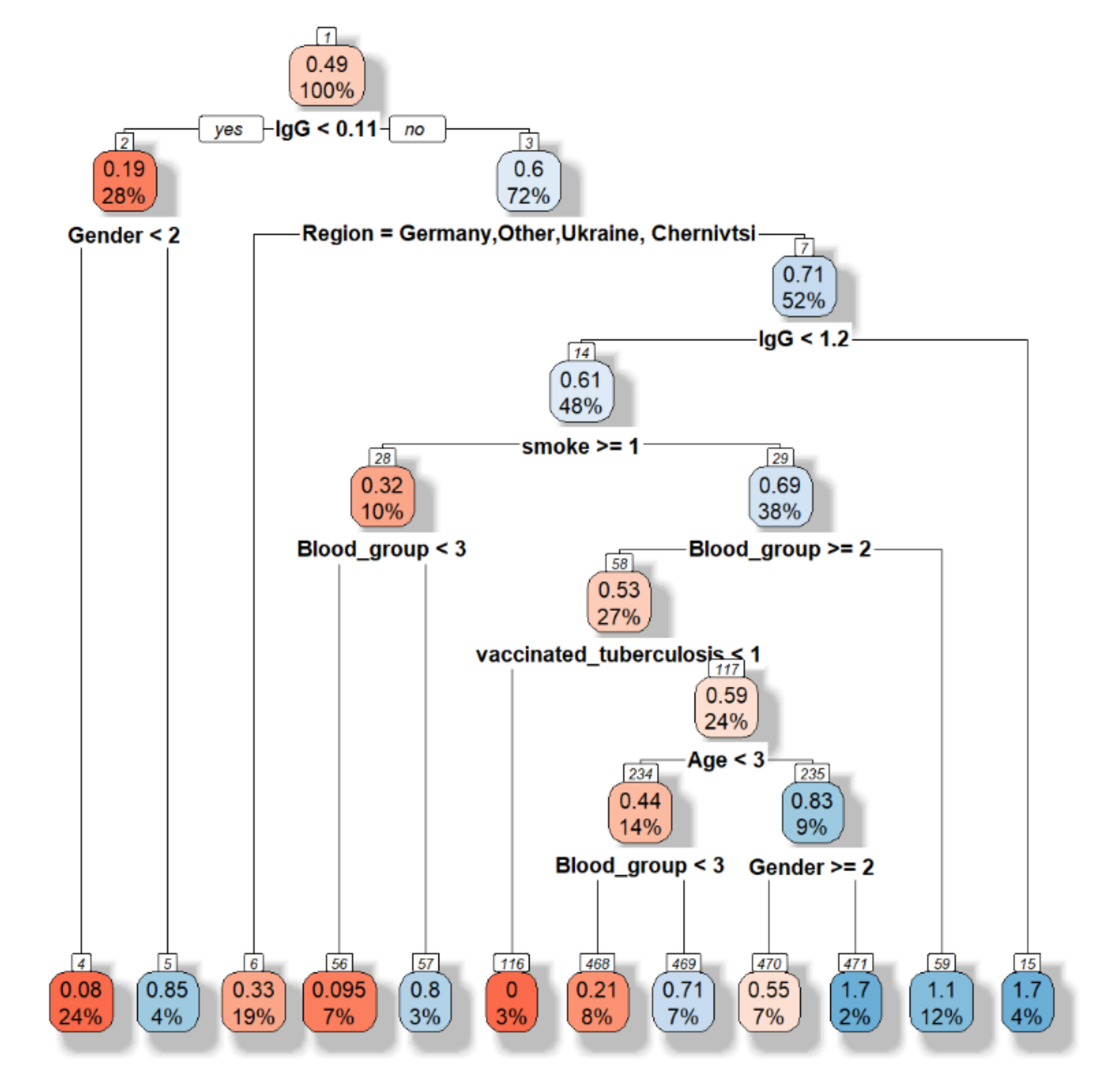
First, the decision tree is built (Figure 7).

The accuracy is equal to 0.5135. However, this model allows choosing the main features as following “Have you had influenza this year”, sex, blood group, region.

Besides the feature selection based on PCA and decision tree shows the different result (Figure 3 and Figure 7), the random forest model will be developed based on all features and grouping features (Figure 3). Five hundred trees with 3 variables tested at each split are built. Mean of squared residuals (MSR) account for dispersions of the actual value of target variable and the estimated value of the target variable derived from linear regression (thus considering the meant of target variable). MSR for the whole dataset and selected features are equal to 0.5067292 and 0.5736409, respectively. Thus, all features are taken into account for future analysis.

Out-of-bag measuring (OOB) is the prediction error of random forests, boosted decision trees, and other machine learning models utilizing bagging to sub-sample data samples used for training. OOB is the mean prediction error on each training sample xᵢ, using only the trees that did not have xᵢ in their bootstrap sample. OOB rate is equal to 16.61%. The confusion matrix is given in

Table 2. Confusion matrix.

	0	1	2	Class Error
0	153	9	17	0.14525139
1	8	88	12	0.18518518
2	1	3	20	0.16666666

.

The biggest error is for class 1 (COVID—yes). It can be explained by differences in IgG and IgM representation (data scatter is between 0.00 and 18.00) in different countries.

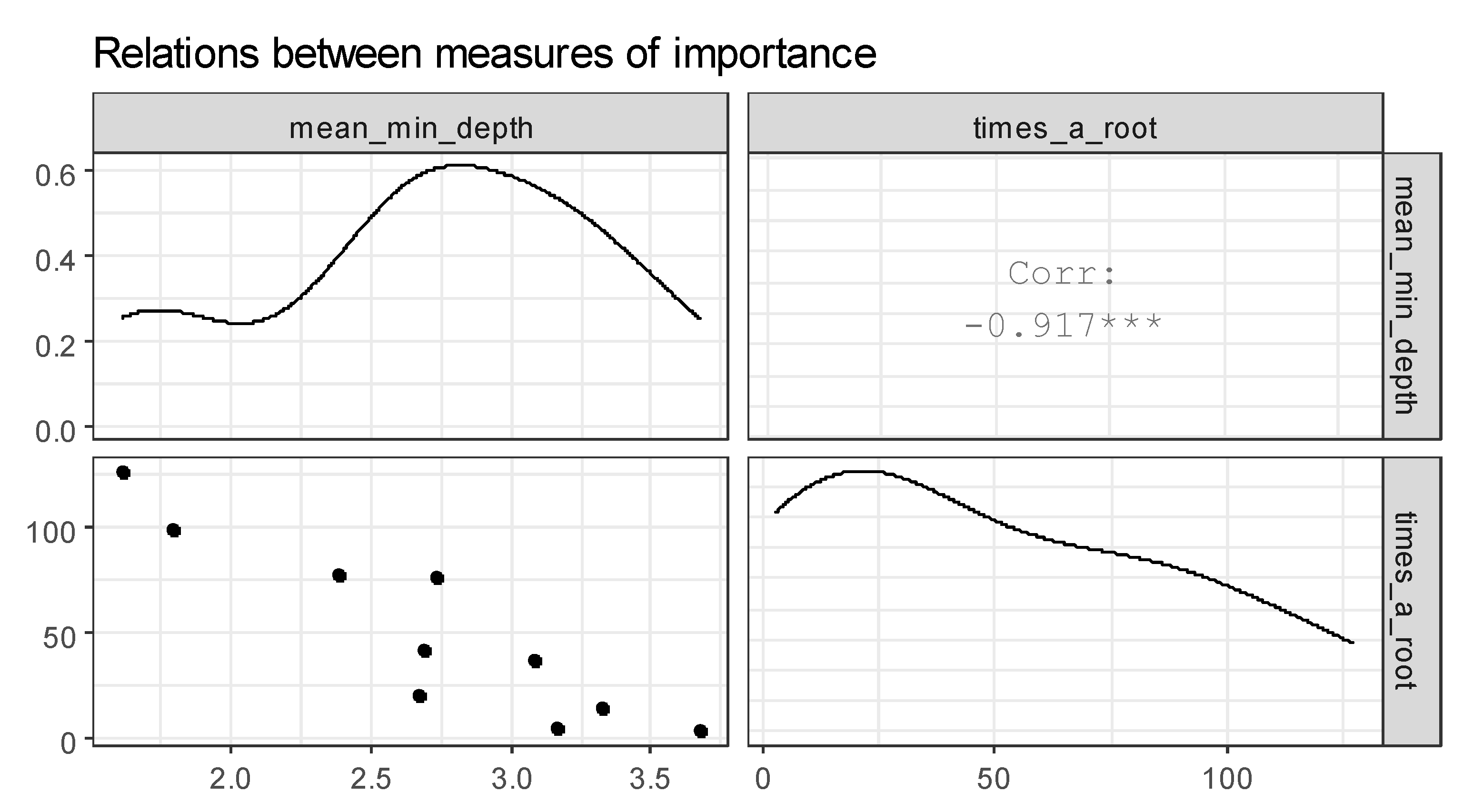
The minimal depth values for all trees in a random forest are given in Figure 8.

The x-axis ranges from zero trees to the maximum number of trees. In each tree, any variable was used for 500 splitting. Therefore, the maximum depth in created trees is for vaccinated influenza. The first level in the biggest part of “poor classifiers” is presented by IgG.

To further explore variable importance measures, we pass our forest to measure importance function and get the following data frame (

Table 3. Data frame based on the random forest algorithm.

#	Variable	Mean_Min Depth	Times_a_Root
1	Age	1.511688	112
2	Blood group	1.620000	111
3	Sex	1.723688	53
4	Had influenza	1.727688	92
5	Smoke	2.030000	79
6	Vaccinated influenza	2.372752	25
7	Vaccinated tuberculosis	2.164000	28

). Age and blood group are the most frequent roots.

Figure 9 represents the plot of selected measures of importance of variables in a forest. The correlation between mean_min_depth and times_a_root is found. From this fact, we conclude that the attributes age and blood type are the most influential on the analysis of the incidence of COVID-19.

After selecting a set of most important variables (

Table 4. Most important variables.

#	Region
1	Age
2	IgG
3	Blood group
4	Had influenza
5	IgM

), we can investigate interactions relatively, i.e., splits appearing in maximal subtrees in accordance with selected variables. To extract the names of 5 most important variables according to both the mean minimal depth and number of trees in which a variable appeared, we have the following result.

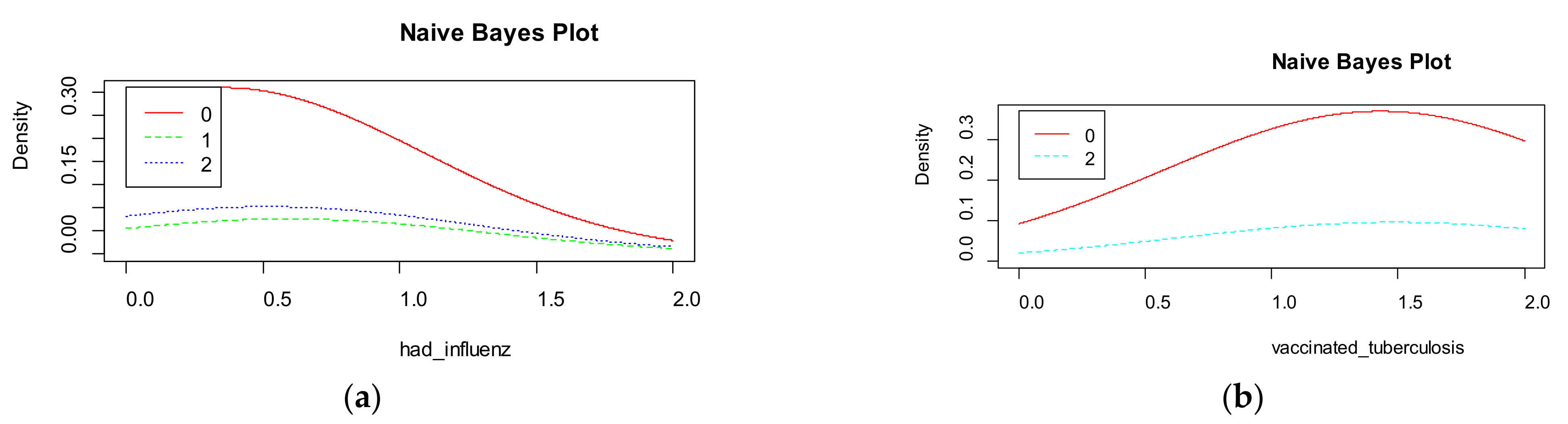
Naive Bayes shows the density for each features in the dataset (Figure 10). The accuracy of naive Bayes is much less than random forest and is equal to 67%. Figure 9 visualizes the marginal probabilities of predictor variables in the given class.

Next step, neural network classification is used. The architecture of the neural network is the following:

• 1 hidden layer and 7 neurons in hidden layer,
• Biases are used,
• Backpropagation as learning algorithm,
• logistic activation function.

The accuracy is equal to 82%.

The following classifiers are used for COVID-19 classification too:

• Support vector machine with lineal kernel shows the accuracy equal to 60.5%.
• Logistic regression for numerical data shows Akaike information criterion (AIC): 37.471. The accuracy is equal to 55.3%.

At the next step of analysis, each classifier is evaluated for:

• whole dataset,
• dataset by countries,
• selected features,
• each cluster separately.

Results of models’ accuracy are given in

Table 5. Models’ accuracy for whole features.

Model	Full Dataset	Filtered by Ukraine	Filtered by Belarus	Filtered by Germany	Cluster 1	Cluster 2	Cluster 3	Cluster 4
Logistic regression	0.553	0.572	0.534	0.544	0.601	0.592	0.610	0.589
Support vector machine	0.605	0.6327	0.570	0.584	0.621	0.694	0.635	0.637
Naive Bayes	0.670	0.693	0.655	0.655	0.674	0.693	0.672	0.692
XGBoost	0.898	0.932	0.860	0.942	0.941	0.945	0.899	0.957
Random forest	0.897	0.924	0.859	0.940	0.932	0.944	0.961	0.925
Neural network	0.820	0.849	0.828	0.79	0.830	0.849	0.8204	0.849
Decision tree	0.513	0.542	0.517	0.492	0.553	0.631	0.612	0.642

and

Table 6. Models’ accuracy for selected features.

Model *	Age, IgG, Blood_Group, Had_Influenz, IgM	Age, Sex, Blood_Group, Had_Influenz
Logistic regression	0.633	0.671
Support vector machine	0.671	0.722
Naive Bayes	0.674	0.732
XGBoost	0.935	0.945
Random forest	0.945	0.934
Neural network	0.832	0.845
Decision tree	0.553	0.631

* Optimal parameters for the investigated methods are shown in Table A2.

.

4.4. Hierarchical Classifier

The importance of variables is different for different methods. It means that dependence between parameters is supported only for part of the dataset. That is why we propose to find the dependence for separated clusters and use this dependence for classification.

We propose the hierarchical classifier as a two-stage algorithm for data prediction. The first stage is clustering; the next stage is classification model building for each separated cluster.

Besides, the hierarchical classifier built on ensemble of k-means and XGBoost shows the best accuracy for clusters 1, 2, and 4. K-means together with random forest is not dominated by the rest of the models in cluster 3. All “poor” classifiers show better accuracy for separated clusters than for the whole dataset.

Therefore, the hierarchical classifier is built as following:

• Using gaps-statistics, the appropriative number of clusters is found. This number is equal to four;
• k-means divides objects by 4 groups; density of distribution is calculated;
• XGboost and random forest are used for each cluster separately;
• Hard voting on the obtained results is provided. Based on it, the class with the highest number of votes will be selected. If votes are the same, the result of the classifier with minimal depth value will be selected.

The accuracy of the hierarchical classifier is given in

Table 7. The accuracy of the hierarchical classifier.

Model	Cluster 1	Cluster 2	Cluster 3	Cluster 4
Hierarchical classifier	0.941	0.945	0.961	0.957

.

XGBoost and random forest algorithms give the high accuracy for the model based on selected features too, but less in comparison with the hierarchical classifier.

5. Conclusions

Thus, it is shown that the study of COVID-19-resistance is now in high demand. Our approach consists of a hierarchical classifier and dependence between COVID-19 resistance and patient’s features estimation. The dataset was collected in different countries and at 29.10.2020 contains 313 observations.

The novelty of the paper is the hierarchical classifier based on the combined usage of unsupervised and supervised machine learning algorithms. The “poor” classifiers based on k-means results are evaluated. The hierarchical classifier is built on k-means, random forest with 500 trees, and XGBoost. Classification for separated clusters gives us higher accuracy on 4% in comparison with dataset analysis. The proposed approach can be used also for personalized medicine decision support in other domains.

The hypothesis that patients with blood group II are more vulnerable to COVID-19 is approved for the collected dataset. This fact can be used in further research.

The features selection allows us to analyze the following features with highest impact to COVID-19: age, sex, blood group, had influenza.

The developed pattern of resistance patient to COVID-19 allows more accurate estimation of new cases based on traditional models such as SSIR, SEIR, SARIMA, etc.

Among the prospects for further research, it is planned to analyze the effectiveness of various ensembles of artificial neural networks to improve the accuracy of solving the classification problem.

References

- Roser, M.; Ritchie, H.; Ortiz-Ospina, E.; Hasell, J. Coronavirus Pandemic (COVID-19). Our World in Data. 2020. Available online: https://ourworldindata.org/coronavirus?utm_campaign=Optimizando&utm_medium=email&utm_source=Revue%20newsletter (accessed on 15 January 2021).
- News. Available online: https://nszu.gov.ua/en/novini/oficijnij-sajt-nacionalnoyi-sluzhbi-zdorovya-ukrayini-staye-19 (accessed on 27 October 2020).
- Тести На Коронавірус—в Україні Зробили Понад Мільйон Тестів ПЛР » Слово і Діло. Available online: https://www.slovoidilo.ua/2020/09/04/infografika/suspilstvo/pandemiya-koronavirusu-skilky-testiv-zrobyly-ukrayini-ta-inshyx-krayinax-svitu (accessed on 5 January 2021).
- Vyklyuk, Y.; Manylich, M.; Škoda, M.; Radovanović, M.M.; Petrović, M.D. Modeling and Analysis of Different Scenarios for the Spread of COVID-19 by Using the Modified Multi-Agent Systems—Evidence from the Selected Countries. Results Phys. 2020, 103662. [Google Scholar] [CrossRef]
- Izonin, I.; Tkachenko, R.; Verhun, V.; Zub, K. An Approach towards Missing Data Management Using Improved GRNN-SGTM Ensemble Method. JESTECH. in press. [CrossRef]
- Jiang, C.; Yao, X.; Zhao, Y.; Wu, J.; Huang, P.; Pan, C.; Liu, S.; Pan, C. Comparative Review of Respiratory Diseases Caused by Coronaviruses and Influenza A Viruses during Epidemic Season. Microbes Infect. 2020, 22, 236–244. [Google Scholar] [CrossRef] [PubMed]
- Charpentier, C.; Ichou, H.; Damond, F.; Bouvet, E.; Chaix, M.-L.; Ferré, V.; Delaugerre, C.; Mahjoub, N.; Larrouy, L.; Le Hingrat, Q.; et al. Performance Evaluation of Two SARS-CoV-2 IgG/IgM Rapid Tests (Covid-Presto and NG-Test) and One IgG Automated Immunoassay (Abbott). J. Clin. Virol. 2020, 132, 104618. [Google Scholar] [CrossRef] [PubMed]
- Muhammad, L.J.; Islam, M.M.; Usman, S.S.; Ayon, S.I. Predictive Data Mining Models for Novel Coronavirus (COVID-19) Infected Patients’ Recovery. SN Comp. Sci. 2020, 1. [Google Scholar] [CrossRef] [PubMed]
- Ivorra, B.; Ferrández, M.R.; Vela-Pérez, M.; Ramos, A.M. Mathematical Modeling of the Spread of the Coronavirus Disease 2019 (COVID-19) Taking into Account the Undetected Infections. The Case of China. Commun. Nonlinear Sci. Numer. Simul. 2020, 88, 105303. [Google Scholar] [CrossRef] [PubMed]
- Caruana, G.; Croxatto, A.; Coste, A.T.; Opota, O.; Lamoth, F.; Jaton, K.; Greub, G. Diagnostic Strategies for SARS-CoV-2 Infection and Interpretation of Microbiological Results. Clin. Microb. Infect. 2020, 26, 1178. [Google Scholar] [CrossRef] [PubMed]
- Ghosal, S.; Sengupta, S.; Majumder, M.; Sinha, B. Linear Regression Analysis to Predict the Number of Deaths in India Due to SARS-CoV-2 at 6 Weeks from Day 0 (100 Cases - March 14th 2020). Diabetes Metab. Syndr. Clin. Res. Rev. 2020, 14, 311–315. [Google Scholar] [CrossRef] [PubMed]
- Yang, Q.; Wang, J.; Ma, H.; Wang, X. Research on COVID-19 Based on ARIMA ModelΔ—Taking Hubei, China as an Example to See the Epidemic in Italy. J. Infect. Public Health 2020, 13, 1415–1418. [Google Scholar] [CrossRef] [PubMed]
- Petukhova, T.; Ojkic, D.; McEwen, B.; Deardon, R.; Poljak, Z. Assessment of Autoregressive Integrated Moving Average (ARIMA), Generalized Linear Autoregressive Moving Average (GLARMA), and Random Forest (RF) Time Series Regression Models for Predicting Influenza A Virus Frequency in Swine in Ontario, Canada. PLoS ONE 2018, 13, e0198313. [Google Scholar] [CrossRef] [PubMed]
- Adhikari, R.; Agrawal, R. An Introductory Study on Time Series Modeling and Forecasting. arXiv 2013, arXiv:1302.6613. [Google Scholar]
- Ez, M.; Ea, S.; Al, F. A SARIMA Forecasting Model to Predict the Number of Cases of Dengue in Campinas, State of São Paulo, Brazil. Rev. Soc. Bras. Med. Trop. 2011, 44, 436–440. [Google Scholar] [CrossRef]
- Dehesh, T.; Mardani-Fard, H.A.; Dehesh, P. Forecasting of COVID-19 Confirmed Cases in Different Countries with ARIMA Models. medRxiv 2020. [Google Scholar] [CrossRef]
- Martinez, E.Z.; Silva, E.A.S.D. Predicting the Number of Cases of Dengue Infection in Ribeirão Preto, São Paulo State, Brazil, Using a SARIMA Model. Cadernos de Saúde Pública 2011, 27, 1809–1818. [Google Scholar] [CrossRef] [PubMed]
- Anastassopoulou, C.; Russo, L.; Tsakris, A.; Siettos, C. Data-Based Analysis, Modelling and Forecasting of the COVID-19 Outbreak. PLoS ONE 2020, 15, e0230405. [Google Scholar] [CrossRef] [PubMed]
- Silva, P.C.L.; Batista, P.V.C.; Lima, H.S.; Alves, M.A.; Guimarães, F.G.; Silva, R.C.P. COVID-ABS: An Agent-Based Model of COVID-19 Epidemic to Simulate Health and Economic Effects of Social Distancing Interventions. Chaos Solitons Fract. 2020, 139, 110088. [Google Scholar] [CrossRef] [PubMed]
- Sakai, H.; Okuma, A. An Algorithm for Checking Dependencies of Attributes in a Table with Non-Deterministic Information: A Rough Sets Based Approach. In Proceedings of the PRICAI 2000 Topics in Artificial Intelligence; Mizoguchi, R., Slaney, J., Eds.; Springer: Berlin/Heidelberg, Germany, 2000; pp. 219–229. [Google Scholar]
- Shakhovska, N.; Izonin, I.; Melnykova, N. Dataset for Covid’19 Resistance Evaluation from Ukraine, Germany and Belarus. 2020. Available online: https://www.researchgate.net/publication/344954442_Dataset_for_Covid19_resistance_evaluation_from_Ukraine_Germany_and_Belarus?channel=doi&linkId=5f9aedc8458515b7cfa7ef90&showFulltext=true (accessed on 15 January 2021).
- Stop Covid’19 Project. Available online: https://covid-72b6d.web.app/results (accessed on 29 October 2020).
- Markopoulos, A.P.; Georgiopoulos, S.; Manolakos, D.E. On the Use of Back Propagation and Radial Basis Function Neural Networks in Surface Roughness Prediction. J. Ind. Eng. Int. 2016, 12, 389–400. [Google Scholar] [CrossRef]
- Mbuvha, R.; Marwala, T. Bayesian Inference of COVID-19 Spreading Rates in South Africa. PLoS ONE 2020, 15. [Google Scholar] [CrossRef] [PubMed]
- (PDF) CoronaTracker: World-Wide COVID-19 Outbreak Data Analysis and Prediction. Available online: https://www.researchgate.net/publication/340032869_CoronaTracker_World-wide_COVID-19_Outbreak_Data_Analysis_and_Prediction (accessed on 27 October 2020).
- Alok, A.K.; Saha, S.; Ekbal, A. A New Semi-Supervised Clustering Technique Using Multi-Objective Optimization. Appl. Intell. 2015, 43, 633–661. [Google Scholar] [CrossRef]
- Shirkhorshidi, A.S.; Aghabozorgi, S.; Wah, T.Y.; Herawan, T. Big Data Clustering: A Review. In Proceedings of the Computational Science and Its Applications—ICCSA 2014; Murgante, B., Misra, S., Rocha, A.M.A.C., Torre, C., Rocha, J.G., Falcão, M.I., Taniar, D., Apduhan, B.O., Gervasi, O., Eds.; Springer International Publishing: Cham, Switzerland, 2014; pp. 707–720. [Google Scholar]