1. Introduction
Competitions in areas like Data Science, Machine Learning, Artificial Intelligence, and Forecasting attract a lot of attention lately for multiple reasons. The practitioners, researchers, and academics not only see an opportunity to put their methods and knowledge to a test, but also compete for enormous monetary prizes many times. Not only that, but, based on their success in these competitions, professionals seek to attract the attention of the big IT companies.
The industry on the other hand utilizes this opportunity to spot talent as well as to identify new tools that outperform significantly the established methodologies. The Netflix challenge
1 is a very characteristic example of the previous decade, but most recently other competitions of the same or even bigger magnitude like the Deep Fake Challenge have been established
2. Although there is a lot of ongoing discussion around competitions of this type regarding their education value [
1], the selection and quality of the data [
2], the incentives [
3], the establishment of an appropriate leaderboard [
4], and many more topics, there is a general agreement that one way or another they contribute to the development of the field they represent [
1].
The M competitions
3 (named after the founder and main organizer—Professor Spyros Makridakis) are a series of competitions that challenge the recent developments and research of forecasting methods and technologies into a set of real world prediction tasks. The goal of the competition is to promote and advance research in the field of Forecasting by providing a competition platform for evaluating and comparing the accuracy of different forecasting methods proposed by both academia and industry. The M-Competitions have a long history starting with the first one at 1982, the M2 at 1993, and the M3 at 2000. The M4 extended the challenge significantly by introducing a large number of time series (100,000) organized in categories of different time granularity (Yearly, Quarterly, Monthly, etc.) and data origin (Micro, Industry, Macro, Finance, Demographic, Other). The M4 advanced the previous competitions as it required the specification of Prediction Intervals (PI) for the provided forecasts. The M5 Competition is scheduled for June, 2020 and explores the use of multivariate and hierarchical data.
Studies that survey and present forecasting methods and their challenges (e.g., missing data) can be found in [
5,
6,
7].
1.1. The M4 Competition Challenges
The M4 consisted of 100,000 time series of Yearly, Quarterly, Monthly and Other (Weekly, Daily, and Hourly) data. The minimum number of observations is 13 for yearly, 16 for quarterly, 42 for monthly, 80 for weekly, 93 for daily, and 700 for hourly series. The 100,000 time series of the dataset come mainly from the Economic, Finance, Demographics, and Industry areas, while also including data from Tourism, Trade, Labor and Wage, Real Estate, Transportation, Natural Resources, and the Environment. The M4 Competition data, as those of the M1 and M3, aim at representing the real world as much as possible. The series were selected randomly from a database of 900,000 series on 28 December 2017.
The goal of the competition can be formulated as follows: Given a training set for each of the 100,000 time series, the competitors were asked to provide a number of forecasts for each one of them. The metric that was utilized for the competition was the Overall Weighted Average (OWA) of two accuracy measures: The Mean Absolute Scaled Error (MASE) [
8] and the Symmetric Mean Absolute Percentage Error (sMAPE) [
9].
These measures are calculated as follows:
where
is the actual value of the time series at the
t-th time interval,
n the number of time periods or observations,
the estimated forecast,
h the forecasting horizon (test set length), and
m is the length of the seasonal periodicity (i.e., twelve for monthly, four for quarterly, 24 for hourly and one for yearly, weekly, and daily data) [
10,
11,
12].
1.2. The M4 Competition Results
The competition received 50+ valid submissions, 18 of which specified prediction intervals (PIs) for all forecasted time series. The results, in summary, are presented in
Table 1. This table features the authors of each method, with their affiliation and finally the percentage improvement over the
comb baseline towards the two under-evaluation metrics (SMAPE and OWA). The
comb baseline method is the simple arithmetic average of Seasonal Exponential Smoothing (SES), Holt, and Damped exponential smoothing and was used as the single benchmark for evaluating all other methods [
12].
Table 2 summarizes information related to a number of forecasting attributes that each method implements. The forecasting attributes that are recorded are: (a) seasonality (a time series characteristic where data present regular and predictable changes), (b) level (the amount of stairs or elevated lines that can be outlined in the data over a period), (c) trend (an aspect that provides info about the growth of observations over a period of time), breakpoints (an unexpected change of forecasting patterns over time), (d) and LSTF (Long Short Term or Memory Forecast: A method’s ability in responding dynamically in past patterns that exist in the data).
1.3. Goals of This Study
The main goal of our study is to investigate and analyze the results of the M4 competition in order to provide a good understanding of the outcome and the potential in the field of forecasting. Specifically, with this article, we would like to shed light on the following questions:
Error Analysis: Where did methods perform well, where did they perform poorly, and why?
Correlation Analysis: Which methods present a high degree of correlation (making errors the same way)? What is the reason for the correlation?
Performance Analysis: Despite their accuracy, what is the performance of each method in terms of computational time? Is the additional computational time reflected in forecasting accuracy?
We would like to note that a comparison between forecasting methods in the M4 competition has been performed by Makridakis et al. in [
12,
21]. In these articles, the authors provide a qualitative analysis comparing the type of each forecasting method (e.g., statistical, ML, combination) and their overall (aggregated) accuracy and ranking. Notable observations from these works are: (i) the most successful methods were the methods that combined statistical approaches; (ii) hybrid (ML, statistical) methods were the best and second best performing methods; and (iii) pure machine learning methods performed poorly, failing to outperform the competition benchmark suite. While interesting articles, to the best of our knowledge, our work is the only study expanding well beyond a qualitative analysis. Specifically, our work is the first and only to perform an in depth error, correlation, and runtime performance analysis to understand why certain methods excel in providing forecasts for diverse timeseries with different periodicities. To perform such an in depth analysis, we obtained the software artifacts of the top-10 performing forecasting methods and re-run the forecasting tasks for all 100K timeseries, studying the error and computational performance of each method at a per timeseries level. We also note that a preliminary version of our work is presented in [
22]. In this work, preliminary results of the correlation analysis are presented.
This study aims to serve as a correlation/computation lens on the methods that participated and excelled in the M4 competition. Including external forecasting approaches to the study would not only be outside the scope of the paper but also unfair, since the methods participating in the experiments below were developed and tuned for the time-series of the M4 competition. On the other hand, as mentioned earlier in this section, data science and forecasting competition and challenges are becoming more important where there is a crucial and urgent need for the community to work on specific scientific/engineering problems. The latest examples of Deep Fakes as well as the Covid-19 challenge
4 underlines this fact and motivates a posteriori studies.
The rest of this paper is structured as follows.
Section 2 presents an overview of the most successful methods in addition to the baselines that were used in the competition. After that, in
Section 3, we present the Error Analysis study that focuses on the characteristics of the time series where the methods failed or succeeded in a great degree.
Section 4 discusses the correlations between the methods in terms of their forecasts.
Section 5 comments on the computational performance of the most successful methods of the competition. Finally,
Section 6 summarizes the paper with some key take-away messages and suggests lines of future work.
2. Methods and Data
In our study, we consider the top-10 performing methods in the competition according to [
21]. The reason for considering the top-10 methods, out of the 100+ submissions received by the M4 competition, boils down to the fact that only 17 forecasting methods were able to surpass the competition benchmark suite, and out of these only the top-10 present a significant improvement beyond the benchmark (presented in
Section 2.1). This shows how difficult the M4 competition is to excel and why the top ranking methods should be studied in depth. For the rest of the paper, we refer to each method as <rank>_<author_name> so we can easily communicate to which method we are referring to, along with its performance. The top-10 methods are displayed in
Table 1.
2.1. The Baseline-Benchmark Suite
In the M4 competition, a baseline approach was introduced in order to have a global indicator of the performance of all methods. That method, named
comb, is a combination of three statistical approaches, namely (a) simple exponential smoothing, (b) Holt’s Exponential Smoothing, and (c) Dampen Exponential Smoothing. Comb has proven to be easy to implement, stable, well performing [
21], and therefore qualifies as a good baseline. It is noteworthy that only a small number of methods outperformed this simplistic but efficient baseline. In order to make this text self contained, and to provide some typical examples of forecasting, we present a brief description of these basic approaches [
23].
Simple Exponential Smoothing: Forecasts are calculated using weights, where weights decrease exponentially as data become older:
where
is the smoothing parameter. In the exponential smoothing method, the predictions lie between the two extremes, the naive
and the simple average
with
T being the time interval, which assumes that all observations are of equal importance, and assigns them equal weights when generating forecasts.
Holt’s Exponential Smoothing: Holt [
24] extended simple exponential smoothing to allow forecasting of series that follow a slope. This method involves a forecast equation and two smoothing equations, one for the level and one for the slope or growth as presented below:
where
denotes an estimate of the level (an elevation constant) and
denotes an estimate of the growth of the series at time
the number of time steps ahead to predict or else horizon,
is the smoothing parameter for level
, and
is the smoothing parameter for slope
.
Dampen Exponential Smoothing: It is a modified version of Holt’s linear method. One of the disadvantages of Holt’s method is that it tends to over forecast, especially for longer forecast horizons. Motivated by this observation, Gardner and McKenzie [
25] introduced a parameter that “dampens” the growth to a flat line some time in the future. Methods that include a damped growth have proven to be very successful, and are arguably the most popular individual methods when forecasts are required automatically for many series.
2.2. The Datasets
The data that we exploit for our analysis are the following:
3. Error Analysis
The ability to predict accurately either in regression or in classification in various data spaces is a common challenge in pattern recognition. Time series analysis is a pattern recognition task that can be modeled as a regression task. Algorithms that are introduced in this field analyze a first (given) part of the time series (the training set) and try to provide with forecasts (predictions) in another (unseen) set (the testing set or horizon as it is being called in forecasting terminology). In many cases, in order to evaluate the accuracy of the forecast, researchers or practitioners tend to apply the forecasting algorithm to a series where the true labels are known. By doing this, they can calculate the error.
The challenge of course is to minimize this error which naturally is defined as the difference between the estimated (forecasted value) and the actual (true) value.
Forecasting can be used to predict data for the next
n steps of time where the step can be anything: a prediction for each one of the next 10 minutes, or each one of the next 12 months. Common fractions of time in forecasting is the Hour, the Day, the Week, the Month, the Quarter, and the Year. These are also the steps (or periods) used in the M4 competition.
Table 3 provides Training/Testing and time-series statistics for each category derived from the M4 time series.
At this point, we denote that, as shown in
Section 1.1, the evaluation metrics of the M4 competition aggregate for each forecasting method the overall error across all 100K timeseries. While this is an acceptable measure to rank forecasting methods to derive a competition winner, it does not provide in-depth insights to how each forecasting method performs. Thus, in this section, we perform an error analysis of the top-10 forecasting methods to study and document (i) (dis-)similar behavior of the forecasting methods; (ii) show where each method had difficulties at a per timeseries basis; and (iii) depict the overall “easy” and “difficult” timeseries, to examine, if the timeseries dynamics (e.g., bursts, distribution change, etc.) could have been foreseen. In what follows, we reveal our methodology, present the results, and eventually discuss the weak and strong points of each method.
We define two measures that we will be needing in our analysis. The first one (Equation (
7)) is the
error percentage of method
j in series
i and is defined as:
With
h, we denote the
horizon i.e., the length to which the testing set extends,
k the index for each time-step in the testing set and
,
the actual and forecast values, respectively. The error percentage values are next utilized in the second measure, the
series error (Equation (
8)) and is defined as:
where
M is the number of methods (the top-ten). This measure then is indicative for the average error of all methods on a specific series
i. One can easily infer that low values indicate good forecasting accuracy for that time series, whereas high values indicate poor forecasting accuracy. This measure therefore is indicative of the difficulty of each series. We calculate these measures for all
N series in a category and create the list with all the series errors
. This list, sorted for each category, is the basis of our error analysis.
We select the easiest four (top four in the list) and the hardest four (bottom four in the list) from each category—then, in order to study the correlation among the top-10 methods, we do the following:
We calculate the
step error percentage (Equation (
9)), for each step
k of the testing horizon. The errors of a specific method
j are then collected in the
error vector of method
, (Equation (
10)):
Eventually, for every method
, we get the per series
error matrix (Equation (
11)) with size
.
We have a matrix like this for all (easiest-four, most difficult-four) series and all the categories, respectively. These matrices are then employed to produce visualizations of error series as in
Figure 1 and
Figure 2. In the following paragraphs, we comment upon these visualizations.
As we have mentioned before, these are the easiest time series and that is evident from all the error lines that we see in
Figure 1. All errors are very close to zero. We also observe that, in many cases, the error lines are very close to each other and almost identical like the series in Daily, Monthly, and Quarterly category. In the Hourly, where there is a lot of variance, we also observe methods that behave quite differently like 8-Legaki, in
#214 and
#315 or 10-Pedregal in
#60.
Figure 2 presents the “most difficult”-four series per category. These are essentially the series where the (top-10) methods performed worst (i.e., had the highest accumulated error). Hence, it could be argued that these are the hardest to predict series. Here, we observe that the errors diverge from the zero value. This is evident in most series. However, in most cases, the error lines are identical with each other like in Daily, Monthly, Quarterly, and Yearly. In the Hourly where there is a lot of variance, we observe methods that behave quite differently like 3-Pawlikowski in
#130 and 5-Fiorucci, 8-Legaki in
#370,
#168, respectively.
At this point, it is noteworthy to discuss the similarity of the error line patterns among the top-10 methods. Most methods, either in the “easiest”-four or in the “most difficult”-four overlap one another in many series. This indicates that, despite their architecture and set of parameters’ differences they use to forecast, they produce similar error line trends. We will study similarities and differences of the top-10 methods in
Section 4.
Moreover, regarding the competition and the performance of the top-10 methods within the above examined series, we notice that the model which came first in the competition (1-Smyl) did not always present the best performance over the competitors. Actually, 1-Smyl presents the worst performance of all top methods in some of the above time series (see #2837 for example). This observation indicates that there is no single solution that fits all time series and there is room for developing ensemble methods that combine the best characteristics of each method. Another approach would be the development of a method that identifies which method is most suitable for each time series, after analyzing its characteristics.
3.1. A Closer Look at the Time Series
We continue the study of the error analysis looking for reasons of why the top-10 methods performed poorly at particular time series.
We use the
error percentage measure (Equation (
7)), calculate it for every method
and series
, and create the
error percentage lists
, (Equation (
12))
These lists are next sorted individually and, for each method (j), we extract the n "most difficult” time series (n = 5 in our case). These are the time-series where the particular method performed poorly (i.e., demonstrated the highest error in comparison with other time series).
Hourly.
Table 4 presents the five most difficult series for the “Hourly” category and the top-10 methods. We observe series
#349,
#130, and
#153 appear in the majority of the methods. However, only series
#349 also appears in the most accumulated error series,
Figure 2a. This observation that series
#349 is in the most accumulated error series and in the individual series leads to inferring that the respective methods (see
Table 4) used a similar feature’s set in the forecasting task.
Figure 3 visualizes the actual time series in two parts: (a) the history/training part that the competitors used to train their model, and (b) the part that they had to forecast (in grey background).
Some important observations related to these results are the following. First, all series display wave-like form both in the training and in the testing area. Second, the sizes of the training sets differ significantly (series #153, for example, has a much shorter training set). Series #349 follows the same wave trend through training and testing. In the testing area, however, these wave characteristics are lost. In series #153, the end point in the training area differs from the respective starting in the testing. Finally, in series #130, the wave amplitude differs between training and testing areas (i.e., the amplitude in the training area is smaller with respect to the testing area).
Overall, from this category, we infer that the main cause of poor performance is because of significant inconsistencies between training and testing area patterns.
Daily.
Table 5 presents the five most difficult series for the “Daily” category and the top-10 methods. We observe series
#1696,
#2214, and
#3329 appear in the majority of the methods. All three also appear in the most accumulated error series,
Figure 2b. Similarly, this observation infers forecasting similarity for the 2-Manso, 5-Fioruci, 6-Petropoulos, and 7-Shaub methods.
In
Figure 4, we observe that series
#1696,
#2214 have smaller training sizes if compared with series
#3329. On the other hand, despite their length differences, they share common trends in the training and the testing area. (i.e., they follow ascending and descending trends in the training and vertical descending lines in the testing). Considering the above remarks and the common attributes they share, one would normally expect forecasting in series
#3329 to be far better than series
#2214. However, both series share common rankings in most methods in
Table 5. In the next section, we will study the relationship of time-series lengths and forecast accuracy.
Here, as also in the previous category (Hourly), the main reason for the poor performance is the discrepancy between training/testing patterns. This discrepancy produces uncertainty and it is unlikely for models to simply overcome without additional knowledge.
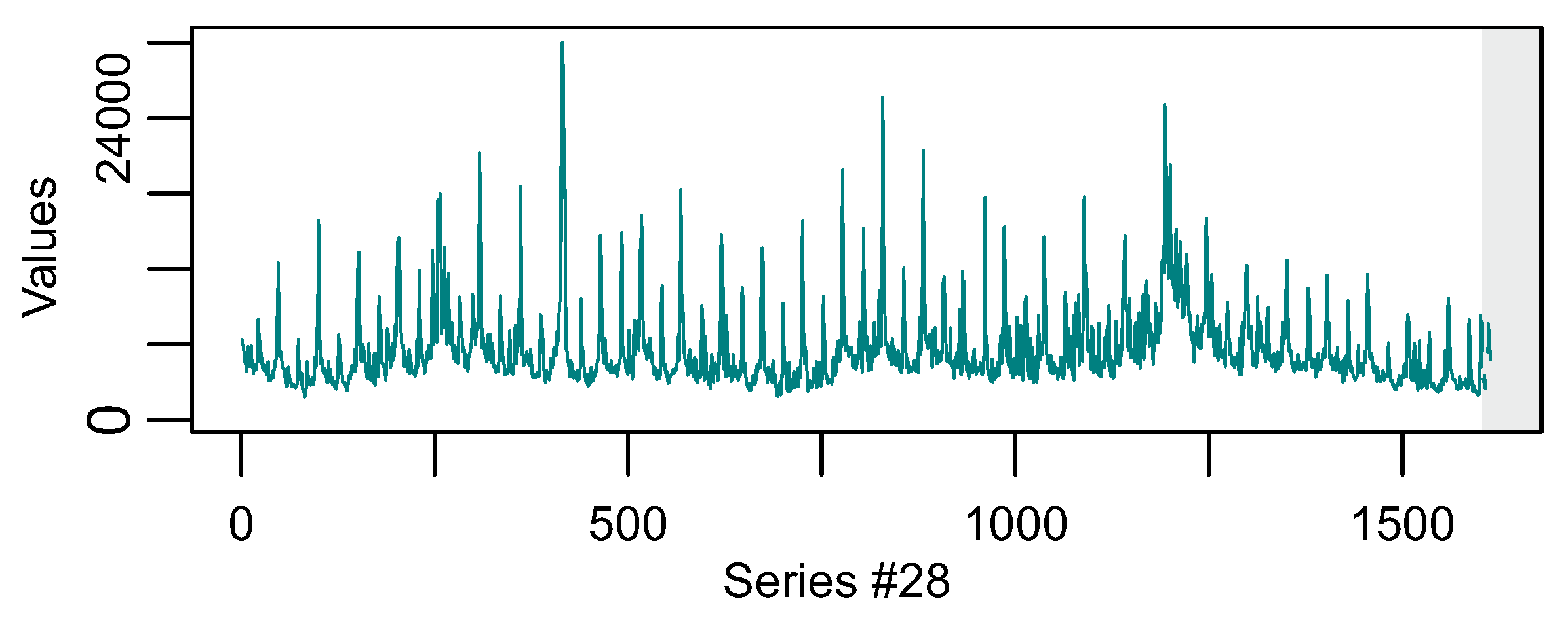
Weekly.
Table 6 presents the five most difficult series for the “Weekly” category and the top-10 methods. Series #28 is the only one that appears in the majority of the methods. Looking back in
Figure 2c, we observe that this series is also among the most accumulated error series. However, it is not in the “most difficult”-five lists of 8-Legaki and 10-Pedregal, but it is the “most difficult” in the lists of 1-Smyl, 2-Manso, 3-Pawlikowski and 6-Petropoulos, since it is ranked first (
Table 6). The fact that there is only one series in these lists leads to the conclusion that, at least in this category, the methods forecast in a different way. This is quite interesting because series #28 displays periodic characteristics throughout the training area and normally forecasting methods
Figure 5 should forecast well without difficulties. We assume that the vertical oscillations and the “learning window” (i.e., the training interval each method employed to forecast) must have been the main reason of uncertainty that obfuscated method’s forecast ability and also caused variance among the top-10 methods.
Monthly.
Table 7 presents the five most difficult series for the Monthly category for the top-10 methods. In this category series,
#39654,
#34726,
#129, and
#14708 appear in the majority of the methods. All four also appear in the series with the most accumulated Error (see
Figure 2d). Looking into
Figure 6 and the respective training/testing data, it becomes quite clear why the top-10 methods performed poorly. This is the discrepancy between the training and the testing patterns. Observing the lengths in series
#39654,
#34726,
#129 and their rank in
Table 7, we can identify the expected correlation between length and accuracy (i.e., the greater the length the better the accuracy). However, this is not the norm, since one would expect forecasting of series
#14708 to be worse than series
#34726 because the latter has larger length. Time-series length is an important attribute that affects forecast. The following section studies this correlation in more detail.
Quarterly.
Table 8 presents the five most difficult series for the “Quarterly” category and the top-10 methods. In this category series,
#9095,
#19147,
#6020,
#12742, and
#2324 appear in the majority of the methods. All five also appear in the series with the most accumulated error (see
Figure 2e). By studying
Figure 7, we infer why the top-10 methods performed poorly in these time series. Extremely short training lengths, nonlinear trends, and discrepancy between training and testing area patterns.
Yearly.
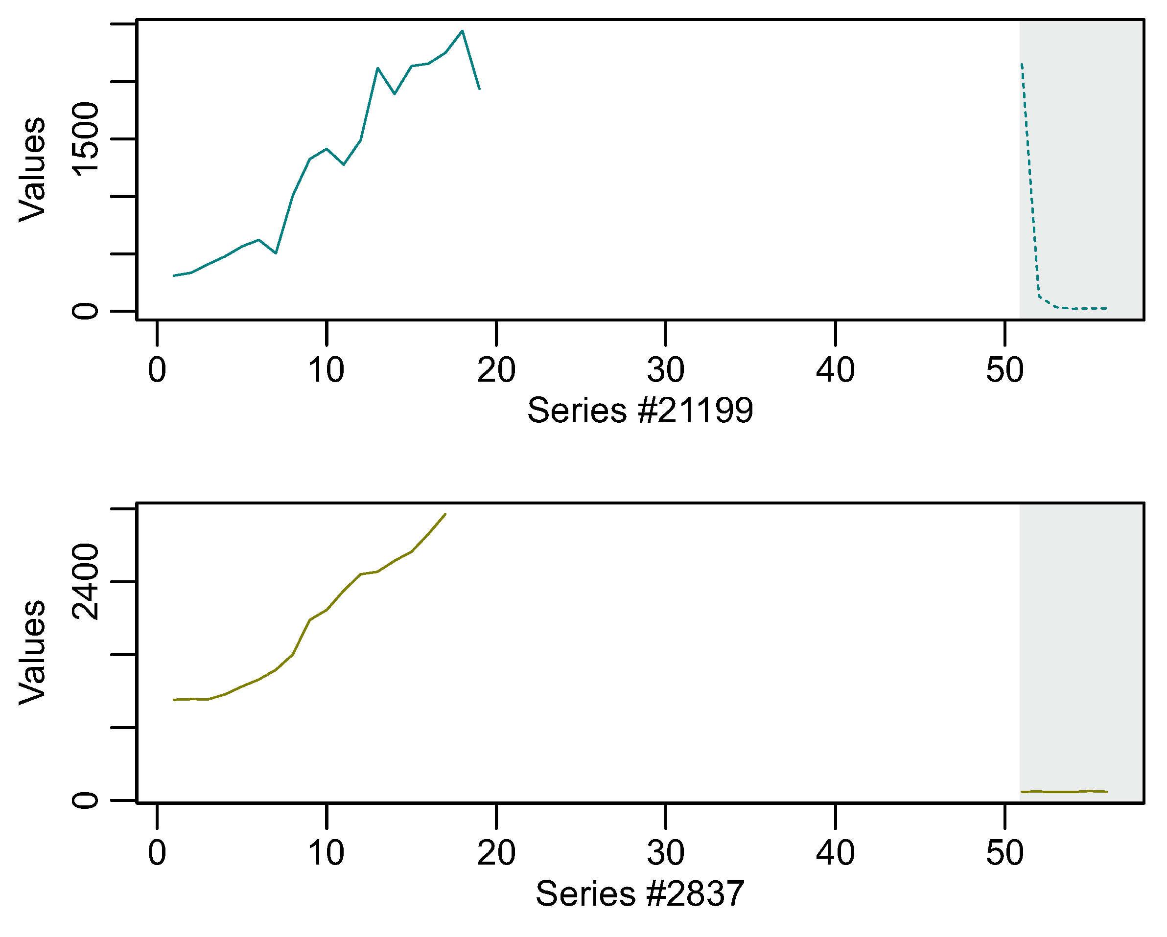
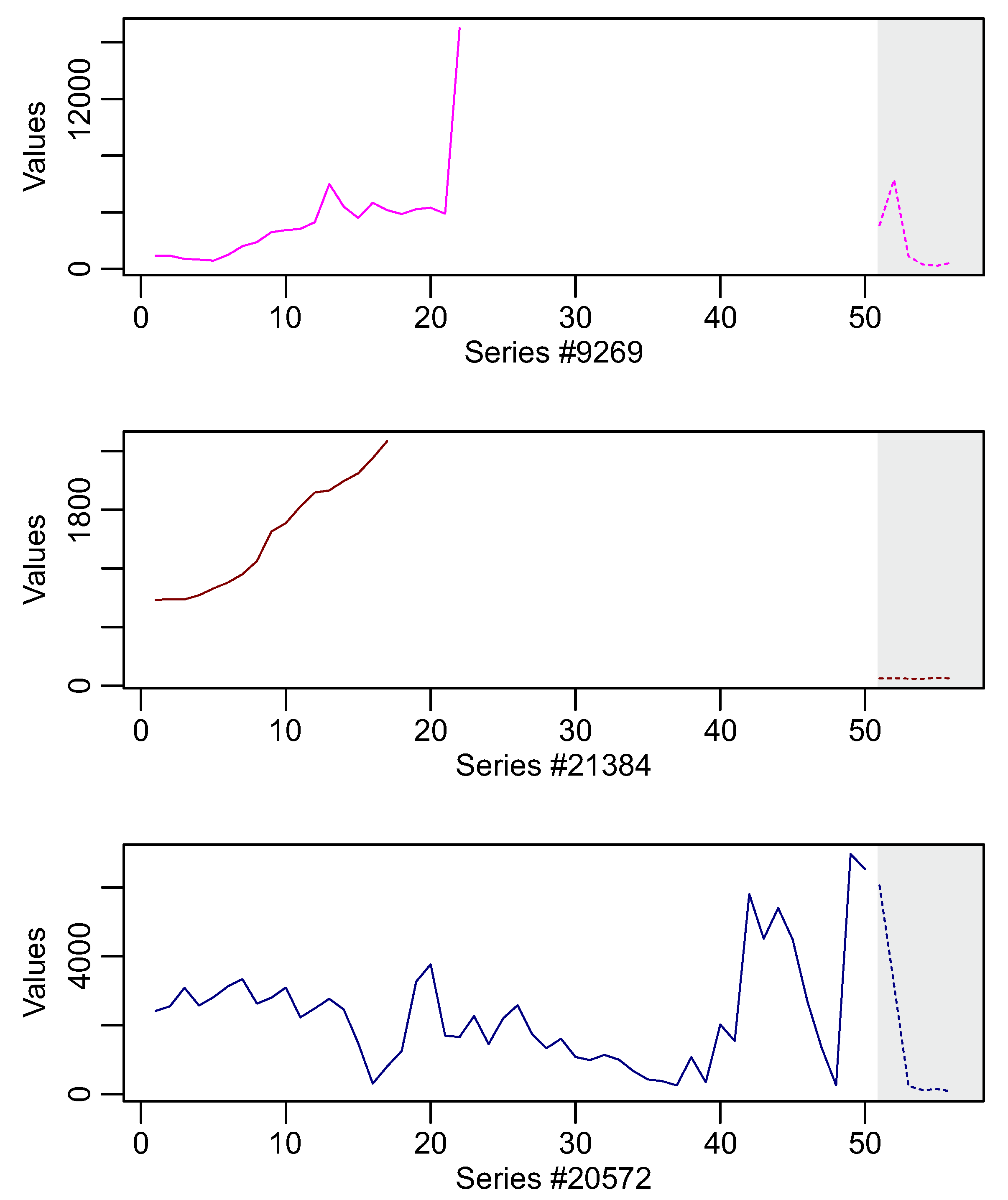
Table 9 presents the five “most difficult” series for the Yearly category for the top-10 methods. In this category, series
#21199,
#2837,
#9269,
#21384,
#20572 appear in the majority of the methods. All five also appear in
Figure 2f. Studying
Figure 8 and the respective time-series in the training and testing areas, we infer observations similar to the previous category, the “Quarterly”. That is, the discrepancy between the training observations and the respective testing. We also notice that four out of five time series are of very short lengths.
It is interesting to discuss at this point where the top-10 methods presented the greatest dissimilarity.
Table 4,
Table 5,
Table 6,
Table 7,
Table 8 and
Table 9 provide this information. We focus on the categories where methods presented the largest variance or dissimilarity among the error series rankings. These dissimilarities are identified at the Hourly and the Weekly category. Regarding the first, the Hourly, we attribute this to the fact that this category had the largest testing length, 48 observations. Consequently, differences in method’s forecasting feature sets could more easily be depicted in this category.
As regards the second, the Weekly, we argue that methods’ dissimilarities occurred because of the wave characteristics of the time-series in this category and the different set of features each method employed to forecast. Recall that, in this category, the number of test data are limited to six observations.
In this sub-section, we studied the most challenging time-series for the six categories (
Table 3). These series were particularly interesting and revealed some of the difficulties the top-10 methods encountered in their effort to provide with accurate forecasts. Overall, the most significant difficulties were observed in short-time series lengths, in the discrepancy between train and test area patterns, nonlinear, non periodic time-series trends and continuity gaps.
3.2. The Effect of the Length of the Time-Series
This section follows up the error analysis and continues with the twenty easiest and the twenty most difficult series for each method. We explore their relation to forecasting accuracy.
We utilize the
error percentage lists (Equation (
12)) and select the easiest-twenty and most difficult-twenty series from each method. Then, we collect their lengths from the M4 dataset and visualize the results.
Figure 9 presents this visualization. In the same figure (right column), we also present the series’ lengths distributions per category.
Prior to commenting on the series’ lengths, we derive from the M4 dataset some statistics, like the minimum and maximum length of the testing data.
Table 10 provides these statistics per category.
Here, we provide some explanations about the aim and scope of the visualization presented in
Figure 9. For each category, there are two figures, one with the easiest time series (according to the collective error of the methods) and one with the hardest time series. In each figure, what is presented is the distribution of the length of these time series. To look at a concrete example, let’s consider
Figure 9a. The first line (orange color) shows the (distribution of the) length of the easiest time series for that particular method (10-Pedregal). Apparently, most of the time series were quite large (most of them at ∼1000 points) and that is the main reason why 10-Pedregal performed well in this category. We have a similar graph in
Figure 9b but for the most difficult time series. In this one, for 10-Pedregal, there are some smaller time-series as well (∼750 points). Now,
Figure 9c is just there to provide an understanding of the lengths in this category.
Starting from the first category (Hourly),
Figure 9a,b, and the overall
Figure 9c, we comment on the following points. In this category, the series lengths are distributed around two only points. Access to the source of the time-series is not available, hence we cannot comment on the reason for this phenomenon. The shortest point contains 700 observations and the longest 960 observations (see
Figure 9c, and
Table 10). In the “easiest”-twenty, the distribution is limited around the longest length 960 while in the “most difficult”-twenty, the distribution spans at both the shortest 700 and the longest 960 series lengths, respectively. In the “most difficult”-twenty
Figure 9b, and the shortest length 700, we observe that methods 10-Pedregal, 9-Dornik, 4-Jaganathan and 3-Pawlikowski scored the lowest frequencies (i.e., they failed in fewer series). However, in the longest 960, nearly all methods scored high frequencies or fails. This observation is quite significant and shows which methods employed different features’ sets for the shortest series lengths.
Moving next to the Daily category,
Figure 9d,e, we comment on the following points. Here, the “easiest”-twenty, distribute across all range of lengths. This is also evident after the study of the overall distributions in
Figure 9f. The greater bulk, however, is gathered around the shortest and the longest lengths. In the “most difficult”-twenty, all methods scored high frequencies around the shortest time series lengths.
After the analysis of the series lengths in the daily category, we infer that series length affects the accuracy.
The Weekly category comes next. We discuss
Figure 9g,h. In this category, there are no significant differences between the distributions in “easiest” and “most difficult” time-series lengths. This is because we notice similar length distributions in both figures. However, in the twenty “most difficult”, methods 4-Jaganathan, 6-Petropoulos, 9-Doornik scored the lowest frequencies in the shortest lengths’ distributions.
The Monthly category is presented in
Figure 9j,k. Here, the “easiest”-twenty distribute across the entire range of length distributions, between
50 and
300 observations (see also
Figure 9l). In the “most difficult” twenty, however, most series are clustered around the shortest lengths. Consequently, in this category, series lengths affect the accuracy.
In the Quarterly category, the distribution of series lengths on
Figure 9m,n are very similar. Because of this, it is difficult to draw conclusions related to the correlation of time-series length and forecasting accuracy.
Yearly is the last category of this study and is depicted in
Figure 9p,q. Similarly as above, in the Quarterly category, there are no significant differences among the series lengths’ distributions.
Overall, in this section, we studied the impact of the series lengths in the forecasting accuracy. From the observations and the comments above, we infer that time series affects accuracy. However, there is no direct relation since we didn’t find such patterns in all categories. Other forecast factors such as those studied in the previous section seem to impact most the forecasting accuracy.
4. Correlation Analysis
In this section, we discuss the correlation analysis which is used to quantify the association between two or more variables. In our case, the association variables are the top-10 forecasting methods. This section aspires to explore which methods behave similarly, which significantly differ, and potentially which could be combined for the purpose of improving the forecasting performance.
We use the
step error percentage (Equation (
9)) and the
error vector (Equation (
10)). Then, for every method
j and series
i, we create the
error matrix (Equation (
11)). Eventually, we have a matrix like this for every category. These matrices are the basis of the analysis in this section.
We apply the pairwise (Pearson’s) correlation algorithm. This is a per series process that produces for each series, matrices of size . The final correlation matrix is the average values produced from the series.
Eventually, we have the final correlation matrix for every category.
Figure 10 visualizes the result of this process for all methods.
From
Figure 10, it is immediately evident that the top-10 ranked methods present weak correlation for the Hourly and Monthly time-series (and partly for the Daily time-series). This is due to the wide range of forecasting values returned by the methods for these particular time-series. This urged us to further investigate how each of the top-10 methods structures its forecasting module.
Specifically, the method 2-Manso is strongly correlated with 3-Pawlikowski, 7-Shaub, 5-Fiorucci, and 10-Pedregal. This is due to the fact that 2-Manso utilizes in its forecasting module a combination of nine statistical and neural network models, including an ARIMA-based model and a Theta-based model which are adopted in 7-Shaub as well. In a similar fashion, 2-Manso is strongly correlated to 3-Pawlikowski and 5-Fiorucci which are both methods also adopting a combination of several purely statistical models. In turn, 5-Fiorucci and 8-Legaki are also strongly correlated, with 8-Legaki embracing a purely statistical forecasting approach by utilizing a Box–Cox transformation and theta forecasting model. Towards this, the method 3-Pawlikowski presents a strong correlation to 7-Shaub and 8-Legaki due to the fact that it embraces an ARIMA model and a theta-model which are evident in 7-Shaub and 8-Legaki, respectively.
Moreover, 1-Smyl presents to be correlated with 4-Jaganathan, 6-Petropoulos, and 9-Doornik, which is inherent to the fact that all these methods exploit forecasting approaches to model season trends that are highly evident in the hourly and monthly time-series. Nonetheless, 1-Smyl appears to be weakly correlated to all top-10 methods for the yearly, quarterly, and monthly time-series. This is due to the unique approach adopted in 1-Smyl where not all data comprising the time-series were used. As the author states “Stepping through 300 years of data to forecast six years seems excessive” and therefore only considered a 60-year horizon for the yearly time-series, a 20-year horizon for the monthly time-series and 40 years for the quarterly time-series.
On the other hand, the method 10-Pedregal is strongly correlated to different methods depending on the time-series type (i.e., yearly, mothly, hourly). This is due to the unique forecasting approach adopted in 10-Pedregal, where different forecasting models are embraced depending on the time-series type. Specifically, for the yearly and quarterly time-series, a theta4 model is adopted with an ARMA model subsequently used on the residuals. As such, for these time-series, 10-Pedregal is strongly correlated to 2-Manso and 8-Legaki, whereas, for monthly, weekly, and daily time-series, 10-Pedregal takes the normalized mean from the best benchmarks introduced by the competition organization, which are pure statistical models, and thus is strongly correlated to methods 2-Manso, 5-Fiorucci, and 7-Shaub. In turn, for the hourly time-series, 10-Pedregal adopts a seasonal model that is also embraced in the forecasting modules of method 1-Smyl, 4-Jaganathan, and 9-Doornik.
As a side note, it must be stressed that a detailed description for methods 4-Jaganathan and 5-Fiorucci were not provided for further investigation.
Figure 11 provides supplemental information from the above correlation study. It depicts the visualization of the average forecasting error percentage matrices, introduced earlier in the pre-processing step. Overall, similarities and differences align with the comments mentioned above for the top-10 ranked methods and the respective categories.
5. Compute Performance Analysis
This section provides a performance evaluation by introducing a comparison of the execution time and resource utilization for the top-10 ranked methods
7. Towards this, we realize a testbed for the performance evaluation comprised of one virtual machine from an Openstack private cloud with the following characteristics: Ubuntu Server 16.04.3, 16 vCPUs clocked at 2.66 GHz with 4KB L1 Cache and 16 GB RAM. To extract the runtime performance of the under-evaluation methods, monitoring probes from the JCatascopia cloud monitoring system were used [
26]. Each method was run independently by utilizing Docker containers
8 to allow each method to be completely isolated and configured according to its specific needs (i.e., software dependencies, library versions, directory paths, etc.). In addition, in our performance study, the software artifacts of all forecasting methods were compiled and run unaltered in order to preserve the integrity of each forecasting method in the evaluation. This entails that the performance is assessed on the whole, meaning that we run the forecasting methods as intended by the competition guidelines where the forecasting methods are applied on all 100K timeseries to derive the evaluation metrics documented in
Section 1.1.
The underlying performance of each method is evaluated towards: (i) execution time, this includes the total time required to read the input, train model(s), compute forecasts, and output results; (ii) memory footprint, this includes the maximum memory allocated to the method; and (iii) CPU and execution mode, this includes the underlying compute and processing model (i.e., single-core, parallel) followed by the method. We note that all evaluated methods indicating a parallel execution mode denote that each time-series is processed independently and therefore training and forecast inference can be scheduled in parallel.
Table 11 summarizes the results of the performance evaluation. From this, one can immediately observe that 8-Legaki is by far the fastest method and is the only method immediately comparable to the execution time of the
comb benchmark. Most importantly, as introduced in
Table 1, 8-Legaki presents a remarkable 4.5% improvement in SMAPE when compared to the
comb benchmark. Furthermore, the difference in execution time between 7-Shaub (uses an ARIMA and Theta model combination) and 8-Legaki (uses a Box-Cox transformation and Theta model) is more than 82 hours, although the difference in their SMAPE is merely 0.2%. On the other hand, the 6th ranked method proposed by Petropoulos et al. (using an ARIMA, exponential smoothing, and Theta model combination) features a 1% SMAPE improvement over 7-Shaub and also a
performance improvement, which partially contributed to the introduction of a parallel execution model.
Performance-wise, one can immediately observe that the worst performers are the 2nd and 3rd ranked methods which feature a forecasting module adopting a combination of 8 and 9, statistical and neural network, models, respectively. Interestingly, 1-Smyl, which introduces a hybrid approach combining exponential smoothing with a recurrent neural network (RNN), presents a remarkable performance improvement and a 2.8% SMAPE improvement over the 2nd ranked method, although 2-Manso actually adopts a combination of eight models. Furthermore, as stressed in the previous section, 1-Smyl significantly reduces the search space in the RNN by not utilizing all the datapoints comprising the yearly, monthly, and quarterly time-series. This computationally offloads the testbed, reduces the total execution time, and most importantly does not affect accuracy; on the contrary, it actually improves accuracy.
Based on the findings of this study, one can argue that certain methods (i.e., 1-Smyl, 6-Petropoulos and 8-Legaki) feature actual and practical potential to power the forecasting needs in various real-world settings, including remote, resource-constrained, and delay-sensitive services (i.e., IoT, edge computing, VR/AR, traffic monitoring). Nonetheless, the wide range of execution times, spanning from several minutes to more than 200 h, for the top-10 ranked methods could potentially indicate a need to introduce a performance evaluation metric in future M-competitions, as more time and resources do not always directly indicate a substantial accuracy improvement.
6. Conclusions and the Future of Forecasting
In this section, we summarize key observations over the top-10 ranked methods which excelled in the M4 competition, selected in this study, and we evaluated their results on a multi-factor analysis: the error analysis, the correlation analysis, and the performance analysis. In the error analysis, we initially studied the easiest four/most difficult four series for all methods and categories. In this first approach, similarities and differences among the top-10 methods were observed and discussed. The most significant similarities were observed for the daily (14), the monthly (18), and the quarterly (8) categories at both the easiest four and the most difficult four series. Most significant differences were observed at hourly for 8-Legaki in series #214, #315 and 10-Pedregal in #60 for the easiest four. Then, 3-Pawlikowski in #130, 8-Legaki in #370, and 5-Fiorucci in #168 for the most difficult four, respectively. We continued the error analysis on the top-10 methods in the most difficult error series individually. The most significant difference was observed at the weekly category. This is due to the fact that the top-10 methods presented the greatest variance for their most difficult error series in this category. Similarities were observed at the daily category for 2-Manso, 5-Fioruci, 6-Petropoulos, and 7-Shaub methods. Next, we studied the relation of the time series length to accuracy. This relation was stronger for all methods at the daily and the monthly categories. The methods of 9-Doornik and 4-Jaganathan were the only ones which scored the lowest frequencies for both the hourly and the weekly categories in their lowest series lengths—an indication that reveals that the feature’s set in these methods considered successfully the uncertainty that comes with the low length series.
At the correlation section, the top-10 ranked methods presented weak correlation for the Hourly and the Monthly series (and partly for the Daily time-series), where a wide range of values were returned. As regards the first, 1-Smyl appears to be weakly correlated to all top-10 methods for the yearly, quarterly, and monthly time-series (in his method, not all data comprising the time-series were used). Finally, in the performance section, we study the relation of the training time to accuracy. Here, 8-Legaki is by far the fastest method and is the only method immediately comparable to the execution time of the comb benchmark. Performance-wise, the worst performers were the 2-Manso and 3-Pawlikowski. These methods employed a forecasting module which adopted a combination of 8 and 9, statistical and neural network, models respectively.
As we already mentioned in the previous section, most of the top-10 ranked methods in the M4 competition employed a combination of statistical methods or a combination of statistical methods with machine learning. However, the method which made significant improvement over the M4 benchmark was 1-Smyl.
In the meantime, and, as the M4 competition was running, many new methods were introduced. Novel approaches were presented ranging from linear differential equations [
27], regularized regression [
28], and of course deep learning approaches like Deep Clustering [
29], Recurrent Neural Networks [
30], Deep Ensembles [
31], Attention Networks [
32], and Convolutional Networks [
33]. All these methods were applied in multiple application domains ranging from weather forecasting to pandemics. Even if Machine Learning methods (e.g., Neural Network based) didn’t perform well in the M4 competition, there was a consensus in the M4 Conference in New York in December of 2018 that there is future in the combination of the two approaches (Statistical and Machine Learning).
1-Smyl’s model architecture and implementation were based on an innovative formula that mainly consisted of two main parts: an appropriate neural network and a combination of statistical models. In general, such model implementations encompass two machine learning characteristics. The neural part ensures global feature extraction and the statistical part achieves local feature extraction. The collaboration of these two approaches in a single unit resulted in an overall improvement on the forecasting task. This improvement can be attributed to the fact that global features took into account patterns in the past, outside the scope of local features. An analysis of the error results over a certain time series showed that there do exist such pattern combinations that can reduce the accumulated error if exploited appropriately. The truncated series technique of 1-Smyl was in line with this spirit. The author exploited a valid past data part along with local patterns in a way that reduced the time step error and contributed to an overall improvement on the forecasting task.
Overall, since prediction is all about reducing uncertainty, such hybrid algorithms that exploit the advantages of deep learning along with the advantages of well known statistic methods can potentially contribute towards better forecasting solutions. There is much potential in the world of forecasting when the new developments of deep learning will be combined with the well-established and well-tested in the real world statistical approaches.


