1. Introduction
The territory of Catalonia has been analyzed by remote sensing from different thematic angles such as forest fire patterns and effects [
1], land use and land cover change [
2], agriculture statistics and abandonment [
3,
4], forest dynamics [
5], or even air temperature [
6]. These works required a considerable amount of time spent in data preparation and organization for requesting and downloading, as well as in correcting it geometrically and radiometrically [
7]. To avoid the repetition of the Landsat imagery processing for each study, the Department of Environment of the Catalan Government and Centre de Recerca Ecològica i Aplicacions Forestals (CREAF) created the SatCat data portal that organizes the historical Landsat archive (from years 1972 to 2017) over Catalonia in a single portal and that provides visualization and download functionalities based on OGC Web Map Service (WMS) and Web Coverage Service (WCS) international standards [
8]. Still, CREAF inverts a considerable amount of processing work on maintaining the portal up-to-date and to incorporate the increasing flow of the new Landsat and Sentinel 2 sensors. The two main reasons are the number of processing steps that the raw satellite data requires to make it useful and the difficulties on organizing a big series of imagery scenes in a way that are easy to manage.
To solve the first issue, United States Geological Survey (USGS) and European Space Agency (ESA) have made a considerable effort facilitating the access to optical satellite imagery, processed up to a level that is ready for immediate use on land studies. Recently, Analysis Ready Data (ARD) is distributed in a processing level that is geometrically rectified and free of the effects of the atmosphere, making it ideal for immediate use for vegetation and land use studies [
9]. Since March 2018, ESA has been distributing the Sentinel 2A and 2B data at 2A processing level (Bottom of Atmosphere Reflectance), which can be directly downloaded from the Copernicus Open Access Hub (
https://scihub.copernicus.eu/) also covering the Catalan area. The downloading process is not only available in the portal, but it is also facilitated by an API that makes the automation of the regular updates programmatically possible. At the time of writing this paper, USGS is only providing Landsat ARD for the USA territory (
https://www.usgs.gov/land-resources/nli/landsat/us-landsat-analysis-ready-data) even if it is possible to request on-demand processing of the Landsat series (4-5 TM, 7 ETM and 8 OLI/TIRS) for other regions of the world, including Catalonia.
By applying successive technical improvements in their sensors, satellites are responding to the user demands in terms of spatial and temporal resolution. Obviously, this increment in resolution is accompanied by an increase in the number of files and/or in file sizes. In the past, it was possible to deal with file names and data volume, but is currently becoming increasingly impossible, even when the small region is needed to study. Data distribution is based on bulky scenes with a long list of file names difficult to classify and maintain, which must be downloaded and processed one by one with Geographic Information System (GIS) and Remote Sensing (RS) software. Creating long time series of a small area might take long processing time in repetitive clipping steps and format transformations. In this situation, extracting a time profile of a single position in the space requires visiting a subset of the long list of files. There is a need for having the remote sensing data organized in a way that it is possible to formulate spatio-temporal queries easily. Current distribution in the form of big scenes is not optimized to respond most of such queries, and the fact that some datasets are growing with a continuous flow of more recent scenes until the end of the operational life of the platform adds another level of complexity. One way of making temporal analysis practicable is to organize or index the data in a way that data extraction of a subset of a continuously growing dataset in four dimensions (two spatial, one temporal, and one radiometric) is fast.
The Earth Observations Data Cubes (EODC) is an emerging paradigm transforming how users interact with large spatio-temporal Earth Observations (EO) data [
10]. They provide a better organization of data by indexing it, faster processing speeds by ingesting scenes as well as improved query languages to easily retrieve a convenient subset of data. The Open Data Cube (ODC) [
11,
12] is an implementation of the EODC concept that takes advantage of the existence of ARD to promote and generalize the creation of national data cubes. The Swiss Data Cube (SDC) is the second operational implementation, after Australia [
13], and delivers nationwide information using remotely-sensed time-series Earth Observations [
14]. As will be described later in detail, by permitting for a local installation of the software and the data, the ODC allows for full control of the data sources and the processes and algorithms applied to them. This is particularly convenient to guarantee total reproducibility of the results obtained when analyzing the data, but it will require an investment in hardware as well as an initial effort on populating the system with the right products. In contrast, solutions such as Google Earth Engine (GEE) provides a cloud environment were multi-petabyte archive of georeferenced datasets that includes Earth observation satellites and airborne sensors (e.g., USGS Landsat, NASA MODIS, USDA NASS CDL, and ESA Sentinel), weather and climate datasets, as well as digital elevation models can be immediately used [
15]. Local or global analysis is possible by adopting GEE programming API that provides build in functions, or by programming lower level code. At the time these lines were written, GEE did not include Sentinel 2 Level 2A imagery [
16] (the product being the focus of the presented work). GEE offers unprecedented computer capacities to the uses, removes the need for the user to design parallel code and takes care of the parallel processing automatically. This means that users can only express large computations by using GEE primitives and some operations that cannot be parallelized in GEE simply cannot be performed effectively in this environment. GEE also imposes some limits and other defenses that are necessary to ensure that users do not monopolize the system that can prevent some user applications [
17].
The ODC provides a good starting point for data organization and data query. Still, using an installation of the ODC requires experience in python programming language and in a set of libraries that the ODC builds on top. The ODC offers a Python Application Programming Interface (API) to query and extract data indexed or ingested by the ODC. This library relays on the Python XArray library that is a data structure and a set of functions to deal with multidimensional arrays that are described with metadata and semantics. XArray internally uses NumPy that is a consolidated pure multidimensional array library. To manipulate the data in the ODC the user needs to be knowledgeable on the ODC API, the XArray and NumPy libraries. In addition, if the user wants to get a graphical representation of the data, extra knowledge on Python graphical libraries is also required. Some examples of practical applications where the ODC could be applied are detecting changes in landscape, tracking the evolution of agricultural fields, or the stability of protected areas. Unfortunately, the technical level of expertise for applications similar to the ones mentioned before relegates the use of the ODC to a subset of RS experts skilled in Python programming.
The first part of the paper demonstrates that the same approach used for national data cubes is also useful for smaller areas such as a province or a region of a country and shows how the ODC can be scaled down to the Catalonia region and further down to the level of an European protected area. This paper also demonstrates that the combination of a modest computer infrastructure with semiautomatic processes allows a single individual to manage a data cube. The second part of this paper proposes some additions to the ODC that make possible the exploration of time series of data for users that have no background in programming languages or scripting widening the potential audience. The solution is based on a combination of OGC WMS and WCS services with an integrated HTML5 web client that performs animations and temporal series statistics. The third part of the paper illustrates how a non-programmer can start exploring the data using the HTML5 enabled MiraMon Web Map Browser, and for example, compute the number of non-cloudy measurements for each pixel of the region, and finally discusses the scalability of the solution in space and time.
2. Scaling Down the Data Cube to a Level of a Province, Region or Protected Area
Catalonia is an autonomous community in North-East of Spain, which extends across 32,000 km2. For about 10 years we have manually build the SatCat Landsat archive that exposes geometrically corrected imagery coming from all Landsat series over the complete Catalan territory spanning from the first Landsat 3 image in 1972 to the current Landsat 8 optical product. ESA was solely responsible for Landsat products in Europe for some time, while USGS is mainly responsible for operating and distributing Landsat imagery. Both organizations have provided data to the SatCat. On top of the archive, we setup a standard WMS service encoded in C and developed using libraries coming from the MiraMon software. To be able to retrieve the data fast, the MiraMon WMS server requires preparing it as internal tiles and at a diverse set of resolutions with an automatic interpolation and cutting tool. In addition, the service also adopts the OGC WCS 1.0 standard for subsetting and downloading. The result is an easy to explore dataset that once presented to the public became widely used both for visual exploration and downloading. To introduce a new scene in the time series, a manual repetitive workflow and protocol was established. The temporal and spatial resolution makes the update of series still manually manageable today. Catalonia is divided in 2 Landsat paths one for the east side (GironaBarcelona) and one for the west side (LleidaTarragona) that are kept separated in two layers to preserve the original scenes. Due to the differences in the number of bands and resolutions of the different instruments, each sensor type is also presented as a different layer. The system benefits from the TIME and extra dimensions concept in the WMS standard to define a product that has a time series composed by several original bands. Due to the intrinsic limitations of the WMS interface that provides pictorial representations of the imagery, the browser is not able to change the visualization of the data or to perform any kind of analysis. To facilitate the time series interpretation an animation mechanism was developed, consisting of requesting individual WMS time frames that are presented to the user as a continuous film. In the next section of the paper, we will present an uncommon way of using the WMS standard used in our new map browser that overcomes these limitations.
With the advent of Sentinel 2A and 2B, we have realized that it is no longer possible to process all incoming data manually with the same human resources. As part of the process of rethinking the workflow of building a Sentinel 2 data series to make it more automatic, we have considered the data cube approach as a way to better organize the data but also as a way to maintain the product up to date with the most recent scenes. We realized that the methodology described by the ODC to setup national data cubes can be used on a region of any size so we decided to build a Catalan Data Cube (CDC) starting by the new data flows coming from the ESA Copernicus program.
As for hardware, we were constrained to low budget alternatives. Instead of going for the last state of the art technology, we opted to use a dual Xeon main-board ASUS Z8NA-D6 with 2 Intel X5675 processors with a total of 12 cores (24 virtualized cores) with 48 GB DDR3 1333 Mhz RAM and four 8 TB disks for about 1500 EUR. After setting up a Windows server operating system, we proceeded to setup up the miniconda environment, the PostgreSQL database, the cubeenv software (the ODC), and the Spyder IDE. The process is fully documented in the ODC website
1.
We wanted to start by importing a Sentinel 2 Level 2A product. The process of downloading the data from the ESA Sentinel Data Hub can be made automatic by combining the wget tool with the instructions for batch scripting provided by ESA
2. There are three steps in the process: First, a wget request to the ESA Sentinel Data Hub to find the resources to be downloaded from the product type S2MSI2A in an interval of time and space. As a result we get an atom file with a maximum of 100 hits. Then we needed to download them one by one with a short script (a Python code) to interpret the atom file (that is in XML format) and to create the list of the URLs corresponding to the granule of each hit and download each individual granule. Each granule is provided as a ZIP file following the SAFE format [
18] that needs to be uncompressed.
The ODC works with a PostgreSQL database to store the metadata about the elements in the data cube but it will keep the image data as separated in the hard drive, only retaining a link to them. In order to import resources in the ODC, specific YAML files containing metadata about the resources are necessary to populate the database. The ODC GitHub provides abundant information and examples on how to create the necessary YAML files and how to index imagery in the data cube for the most common products. Two types of YAML files need to be created: A product description for the S2MSI2A product as a whole (mainly specifying details about the sensor and the bands acquired by it) and files that describe the peculiarities of each granule (mainly in terms of spatial and temporal extent). ESA has only recently distributed the S2MSI2A product (since March 2018) so no example of the description of it has been found. We created it ourselves following a YAML file for scenes generated ad-hoc with the Sen2Cor software that produces a very similar SAFE file structure. We also used a Python script that transforms a SAFE folder result from a Sen2Cor execution into a YAML file describing the granule peculiarities that we could adapt to the product generated by ESA. Once we had these YAML files, we were able to index the granules into the data cube. By indexing this kind of data the ODC still relies on the original JPEG2000 formats. JPEG2000 format is designed for high compression and fast extraction of a subset but it still requires some time to decompress each scene, making it not appropriate for queries requiring big time series that results in too slow responses for the ODC API. Fortunately the ODC offers a solution called ingestion. The ingestion process creates another product in the data cube that automatically converts the JPEG2000 files into a tile structure composed by NetCDF files in a desired projection. The ingestion process offers the possibility to mosaic all granules of the same day in a single time slice reducing fragmentation of the Sentinel 2 granules. In the current implementation of this functionality (called ‘solar day’), the process does not take any consideration on which is the best pixel and covers one image with the next, which is something that could be improved in future versions of the ODC software. The ingestion process can be repeated to add new dates in a preexisting time series as soon as they become available and integrated in the data cube into a fully automatic batch process.
Once this process is completed, the data is perfectly organized in the data cube and can be accessed in an agile manner. The cubeenv Python API allows for writing Python scripts that extract a part of a time series as tiles and represent them on screen by using matplotlib. In practice, the data cube offers a spatio-temporal query mechanism that does not require any knowledge about file names, folder structure, or file format. The result is an array of data structures, one for each available time slice. The number of slices in the time series and the dates associated with them is determined by the API. The Python API is a very useful feature to test the ingested data and ensure that all data is correctly available. Some examples on how to do so are provided as Jupyter notebooks in the ODC website. Using the Python library, data can be exploited by analytical algorithms generating new products, which can eventually be reintroduced in the data cube. That might produce great results but the need for Python skills makes it too complicated for most of the GIS community or the Catalan administration and inaccessible to the general public.
To import the Sentinel 2 product for Catalonia in the CDC for the available period from March 2018 to March 2019, involved the download of 1562 granules (204,386 files) resulting in a volume of 1.18 TB (1.301.116.256.901 bytes) of the original scenes in JPEG2000 format that required a downloading and indexing time of about 258 h. Once ingested, it resulted in 132 scenes in a volume of 816 GB (876.598.015.657 bytes) and distributed in 6093 NetCDF files requiring an ingestion time of about 23.4 h.
3. Adding Easy and Interoperable Visualization to the Data Cube
Another Python script was prepared that retrieves the data cube tiles and convert them into the MiraMon server format at a variety of resolutions. The script determines the number of time slices that the data cube can provide at that point in time and it is able to detect if a certain time slice was already prepared in a previous iteration or needs to be prepared now. For each time slice, if the preparation is successful, the script is also able to edit the server configuration file (that is an INI file) to add it to the WMS server and the web map client configuration file (that is a JSON file) to add a time step making the whole update process fully automatic.
Actually, the ODC provides support for WMS services by using the
https://github.com/opendatacube/datacube-ows code. Nevertheless, in this development we wanted to take advantage of a new functionality that we have recently developed in the MiraMon server and map browser for the ECOPotential project: MiraMon implementation of the WMS OGC Web Services serves imagery in JPEG or PNG for standard WMS clients as well as in raw format where the arrays of numeric values (original data) of the cells is transmitted directly to the client (we call it IMG format). The use of a raw numerical format opens a myriad of new possibilities in the client side. Now the map browser JavaScript code is able to request IMG format asynchronously (with AJAX) and get the return as a JavaScript binary array (new characteristic in HTML5). HTML5 also adds support for a graphics library that works on an area of the screen that is called canvas. In the canvas, we can get access to each pixel of the screen area and modify it. Binary arrays are dynamically converted into arrays of RGBA values that will then covering the whole canvas area. The conversion can be as complex as we want, ranging from applying a grey scale color map, creating an RGB combination from 3 bands (3 WMS binary array requests), and up to a complex pixel-to-pixel operation involving several bands and thus many WMS binary array requests [
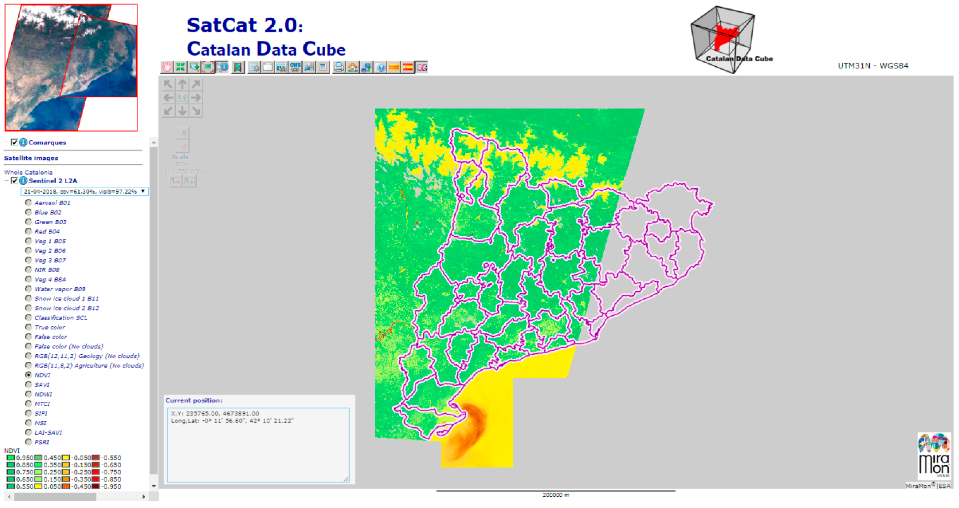
19]. Our CDC WMS client can be accessed at
http://datacube.uab.cat/cdc/ (see
Figure 1). The description of most of the functionalities implemented in the map browser is out of the scope of this paper that will only focus on the time series analysis.
4. Exploratory Analysis of Time Series on the Catalonia Data Cube
In implementing the map browser of the Catalan Data Cube we have gone even further in the use of binary arrays by exploring the potential of using an array of arrays in supporting time series visualization and analytics. A time series is a multidimensional binary array in JavaScript allowing for the extraction of data in any direction of the x,y,t space including spatial slices, but also temporal profiles and 2D images where one dimension is time.
4.1. Summarizing Scene Area and Cloud Coverage of Each Scene
The first thing we did was to generate a list of temporal scenes that could be more meaningful for the user. While downloading data from the Sentinel hub, we are only accepting granules that have less than 80% of cloud coverage. If we combine this with the fact that Catalonia is only covered partially with a single granule and that both Sentinel 2A and 2B are integrated in a single product; it is really difficult to anticipate the real coverage of each daily time slice, if the user is not proficient in the distribution of the satellite paths. For this reason, the list of scene names is a composition of the date, the percentage of the area or interest (a polygon that includes the Catalan territory) covered by scenes with less clouds than CDC limit (80% or less) and the percentage of area covered by scenes that shows the ground (not covered by clouds). In this way, we can differentiate a scene that only covers a small fraction of Catalonia, but with the available part mostly “visible” (not covered by clouds), so it can still be useful to study the small areas as a continuous extent (see
Figure 2).
4.2. Animation of the Temporal Evolution and Temporal Profiles
The main window of the map browser allows showing one scene at a time (see
Figure 1). To perform time series analysis, we have included a new window (that can be opened by pressing the video icon:

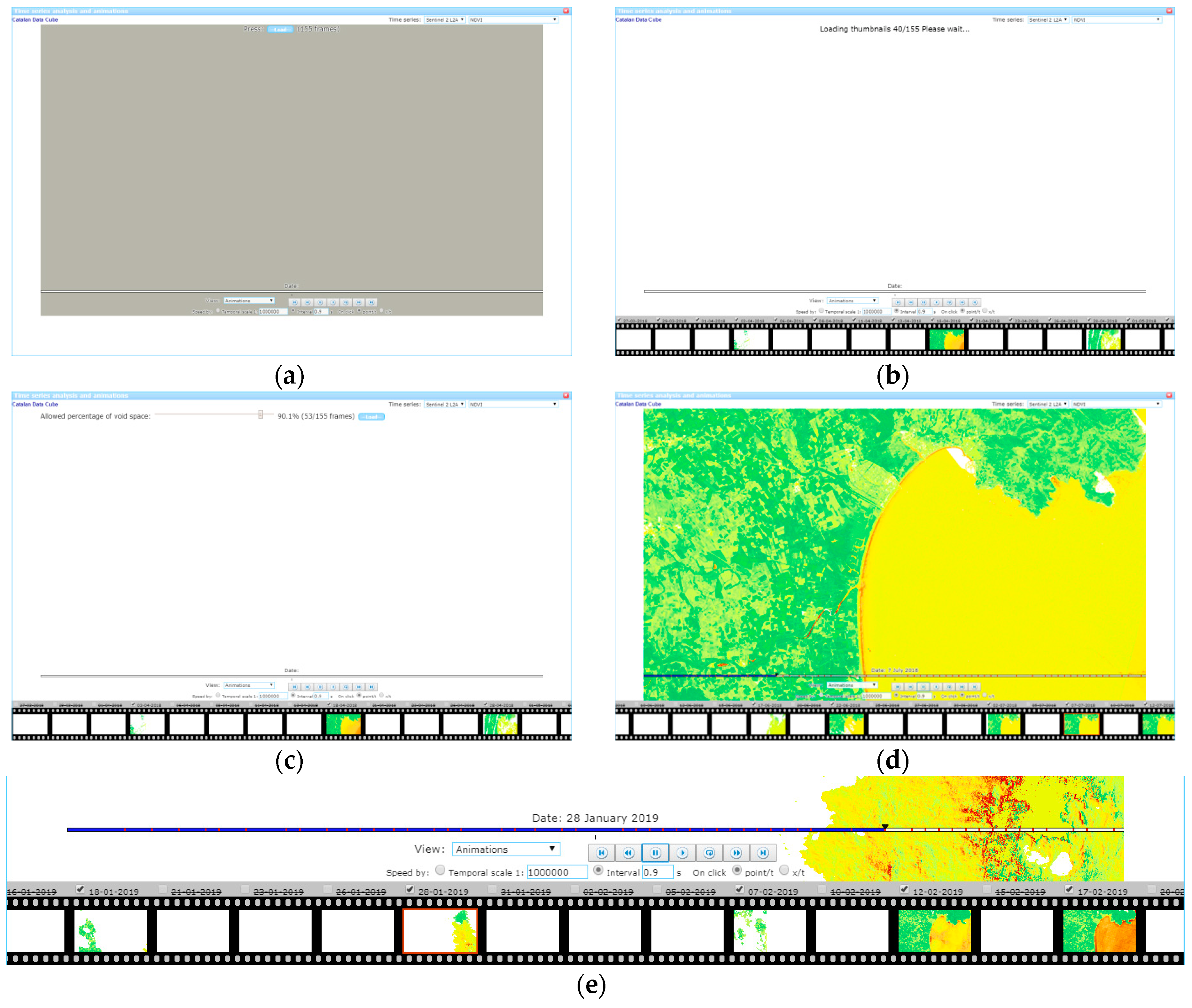
) where the set of time slices of the area defined in the main window will be requested, visualized, and analyzed. For each time slice, the components are downloaded, saved in memory and rendered in a HTML independent division (HTML DIV) that contains a canvas. Creating the animation effect is as simple as hiding all divisions and making visible one of them in sequence (see
Figure 3e). Modern browsers are fast in doing this kind of hiding operations allowing for speeds higher than 10 frames per second, thus resulting in a quite convincing video effect.
In the case of the CDC, downloading and saving the time series binary arrays is a stress test for both the web browser and the map server. Indeed, a time series from a year will involve about 140 scenes that will result in up to 140 WMS GetMap requests of individual time slices, if we are visualizing a band, or 280 WMS GetMap request if we visualize a dynamically generated NDVI. In a state of the art screen the map requires 1500 × 800 pixels or more; and considering that each pixel is represented by 2 bytes (short integer binary array), this will require transmitting a total of 310 MB of uncompressed information for a single band and 620 MB for an NDVI. The situation is partially mitigated by the use of RLE compression during the transmission, but still a considerable amount of data is transmitted from the server to the client. Another factor introduced to mitigate the situation was to consider that, due to the number of scenes having a partial coverage, requesting a time series of a local area will necessarily result in some scenes completely blank. The map browser turns this into an advantage by initially requesting only small quick looks of the scenes (see
Figure 3a,b). This is going to increase the user experience by representing a pre-visualization of the time series in the form of a film, and it is also useful for calculating an estimation of the percentage of nodata values of the area in a certain time-slice. If the quick look is containing nodata values only, it is automatically discarded. Moreover, by operating a slider, the user can then decide to download only the scenes that have a minimum percentage of information in them, reducing the need for requesting unnecessary bad images at full screen resolution (see
Figure 3c,d).
After the user has decided about the accepted percentage of coverage (and presses the
Load button), all the WMS GetMap requests at screen resolution start. Once the images have been downloaded and the multidimensional binary array has been completed, an animation begins showing the sequence of scenes (as the “Animation” option, by default, is selected in the dropdown list on the temporal analysis control, as shown in
Figure 3e).
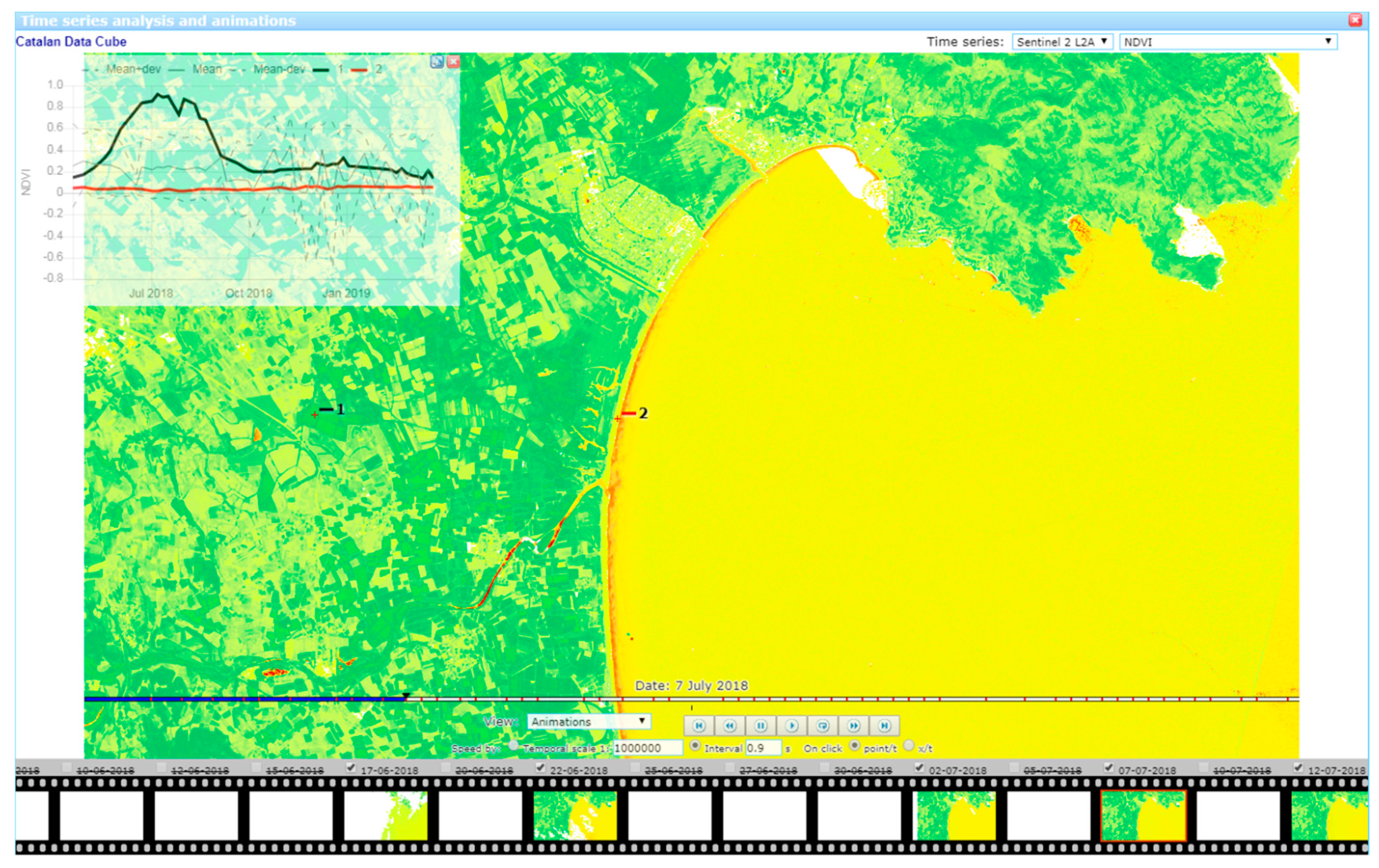
By default, the
On click option is set to point/t and thus when the user clicks on any part of the image, a temporal profile diagram of this point is shown. The profile of the point is presented with the time evolution of the spatial mean value of the pixels from each scene (grey solid line), as well as the mean ± standard deviation as a reference (grey dashed lines). The user can continue clicking in the screen to add temporal profiles of other pixels to the graphic (see
Figure 4). These profiles can be copied to the clipboard as tab separated values that can be later pasted in a spreadsheet for further analysis.
4.3. Temporal Statistics
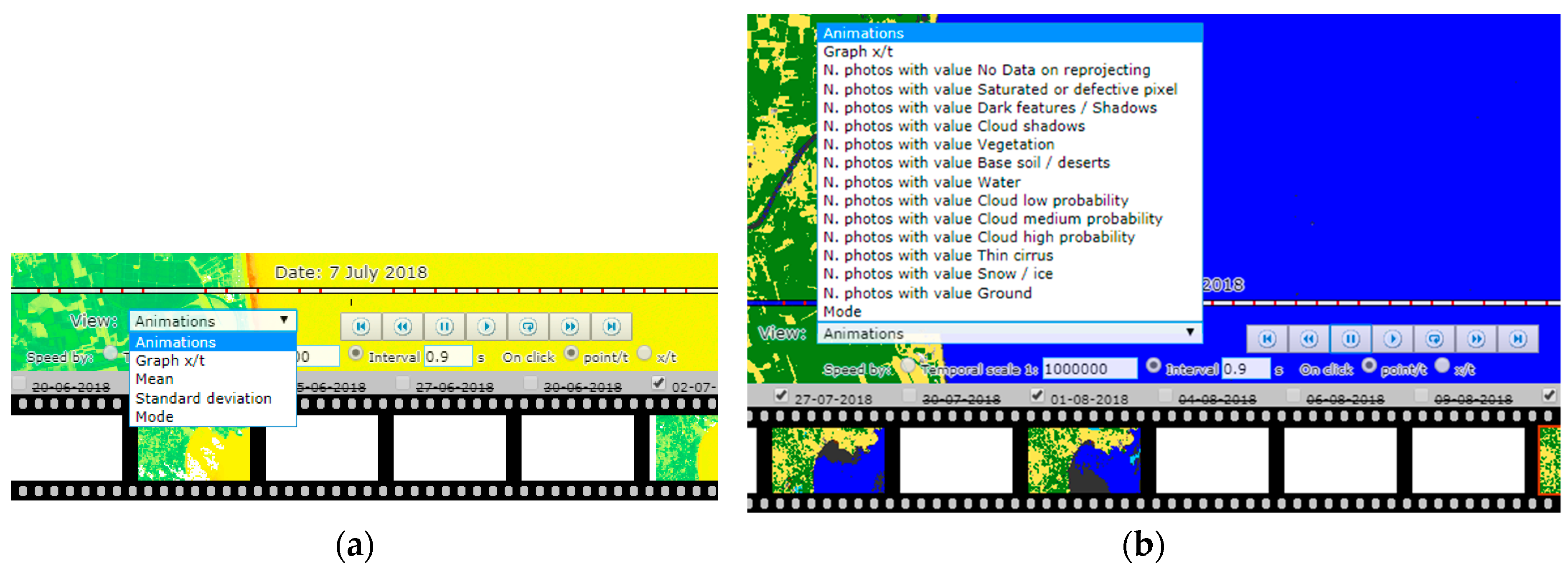
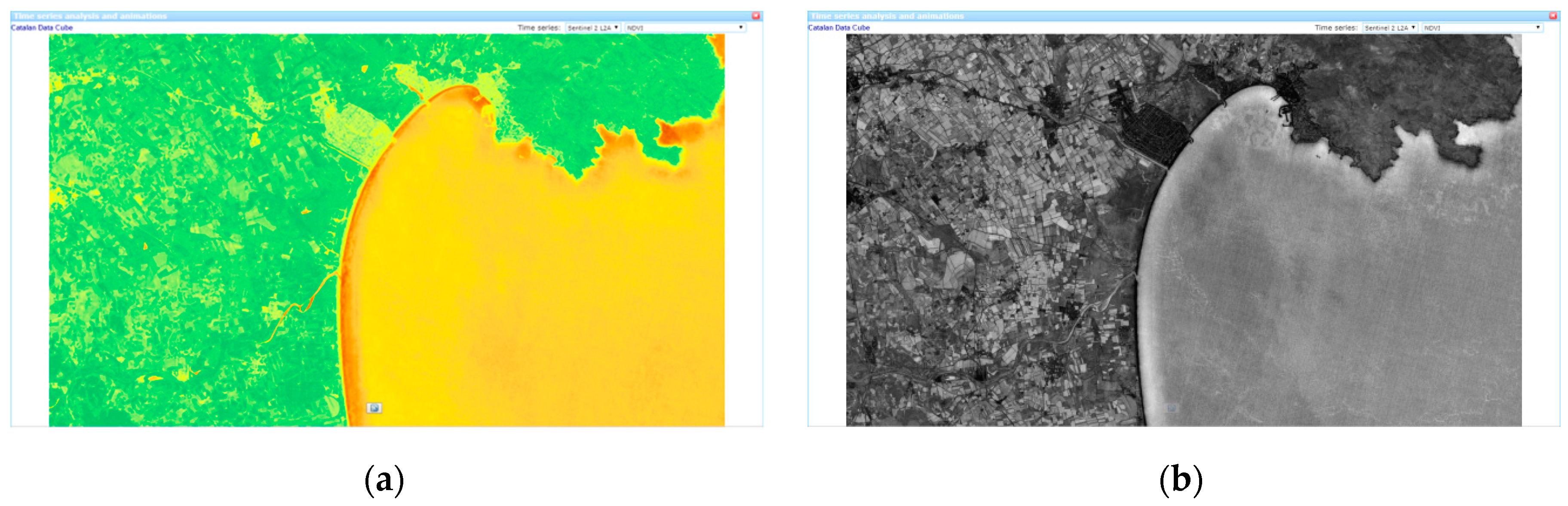
Having a multidimensional binary array in memory opens the door to expand the temporal analysis possibilities. To demonstrate some of them, we have implemented initial statistics, available through the dropdown list
View in the temporal analysis control area. For quantitative values, we can calculate the mean, the mode and the standard deviation of each pixel of the set of scenes resulting in a new image (see
Figure 5a). For categorical values, it is possible to calculate an image that represents the number of scenes, which contain a particular class or the modal value of the time series (see
Figure 5b).
As an example, mean and standard deviation for NDVI are shown in
Figure 6. The mean NDVI is useful to see the overall behaviour of a certain area, and thus being able to identify some covers. Moreover, an overall image representing the amount of variation of a variable can be created by applying the standard deviation expression to each pixel of the time series. The result is an image that has low values in pixels that remain constant over time and high values in pixels that have more variability over time. In an NDVI time series the standard deviation is represented in a grey scale, where white colours represent agricultural fields that have big dynamics in NDVI, grey values are stable forest areas, and dark values are invariant human built environments (such as cities, roads, and paths) that have a much more constant NDVI value over time.
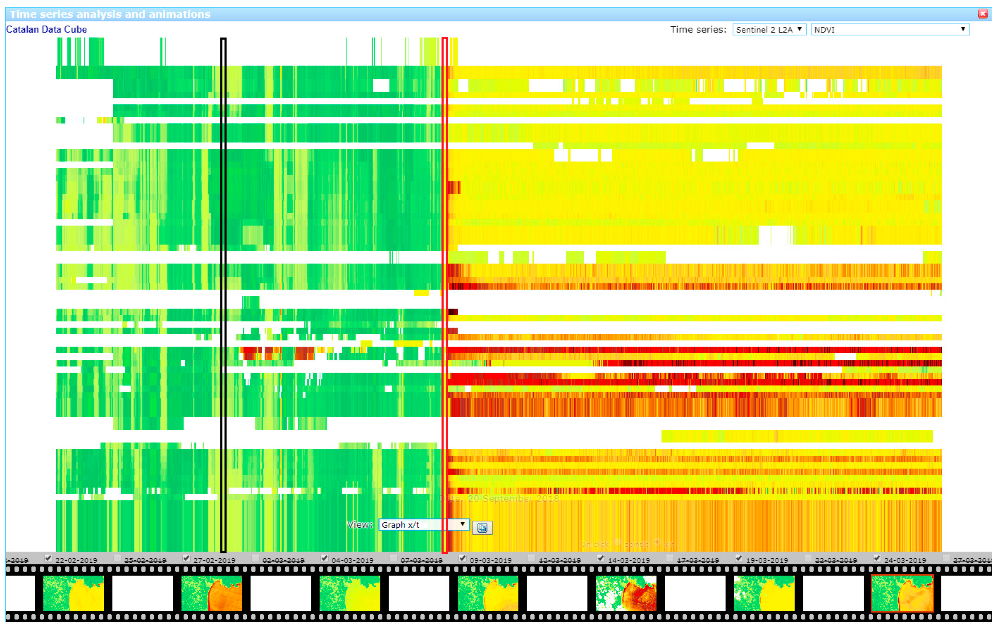
Another interesting addition is the possibility of generating an x/t graph. On this view, a 2D image is formed by selecting a horizontal line in the animation (
Y coordinate that will remain constant) and representing an image where each row is the selected
Y line in one scene. In the resulting 2D graph, time progresses down and “vertical changes” in color reflect changes over time (see
Figure 7). White patches are nodata values present in some of the images in the selected horizontal line. In the future, other time series derived statistics will be incorporated.
4.4. Coverage Evolution in Catalonia along First Year of Sentinel-2 Acquisitions
Sentinel 2 level 2A product generated and distributed by ESA incorporates a categorical band (Scene Classification map, SCL) that classifies the pixels of each image in 12 classes (using L2A_SceneClass algorithm
3). This is particularly useful to estimate if a pixel actually represents the ground or is not very meaningful because it is a missing value, a saturated pixel, or it is covered by clouds, shadows, etc. In the map browser, it is possible to generate a dynamic band that reclassifies all categories that represent a valid value for “ground” (i.e., vegetation, non-vegetated—i.e., bare ground—, water and snow or ice) as a single category. This virtual band will be dynamically computed for all time scenes when needed. Then, in the temporal analysis window, we will be able to see the temporal evolution of this category as well as to generate an image representing the number of scenes that contain the “ground” category (see
Figure 5b). Due to the swath of the Sentinel 2A and B, many scenes partially cover the Catalan territory, a situation that is modulated by the cloud presence, which is more frequent in some regions. The image gives us the actual level of Sentinel 2 imagery recurrence for each part of Catalonia (see
Figure 6).
The result visually reflects that the east part of Catalonia and the North-West part only had about 20 samples in the first year of acquisitions (less than one sample every 15 days). The South-West part presented an average of 40 samples. The central part of Catalonia had more fortune with at least 60 samples, but it is the lower left part of the center area the one that received the maximum number of samples with up to 86 samples (about a sample every 5 days). This is an interesting result that suggests that future efforts in temporal analysis of Sentinel 2 data over Catalonia should focus in the lower left part of the central area, where the temporal resolution is higher and we should expect a better accuracy. This is particularly important for phenological studies that are looking for changes in the vegetation status that can suddenly happen in only 2–3 days (for example the start of the growing season). Sample availability is highly correlated with the common area between orbits that dramatically decreases the revisiting period in certain areas according to its distribution. This is the main reason for the high values in the central part of the image in
Figure 8, as this area is the overlapping between the swaths of the 051 and 008 orbits (see
Figure 9a,b). Moreover, the sample availability is also related to cloud coverage, thus we can assume some relation to annual rainfall.
Figure 9c shows a map of the mean annual rainfall in Catalonia where we can see a certain spatial correlation with the image availability: In certain areas, it is lower (marked by a blue polygon) than in others (marked by an orange rectangle) (see
Figure 9a) as they correspond to areas with higher rainfall (in blue in
Figure 9c) and lower rainfall (in reddish in
Figure 9c), respectively.
5. Discussion & Perspectives
5.1. Can We Apply the Methodology to Other Regions?
As we have explained before, the approach described in this paper was designed with the aim to make the Sentinel 2 imagery collection automatic for Catalonia and to build the CDC. Nevertheless, the same methodology is
a priori applicable to any other region. To demonstrate this, we have deployed another data cube for the protected areas in the H2020 ECOPotential project (
www.ecopotential-project.eu). In ECOPotential, we provide 25 protected areas with the available remote sensing data and derived products that can be used by protected area managers in their maintenance tasks and their decision making processes. To make data exploration easy, we also used an integrated map browser (maps.ecopotential-project.eu) that allows selecting the protected area, and then browse to the data prepared by the different ECOPotential partners. We called it “Protected Areas from Space”.
In ECOPotential we have also experienced the difficulties in retrieving, storing and sorting the relevant information. Due to the heterogeneity of the sources and products, each addition needed to be understood in terms of format and data model, analyzed for the best representation in terms of colors and legends and integrated in the browser. Variety was the most challenging aspect of this big data problem. In the end, this resulted in the largest map browser our organization has ever prepared, with a total of 277 different layers distributed among the 25 protected areas (each layer can present more than one variable and, in many cases, several time frames). However, when trying to incorporate Sentinel 2 we faced the problem of volume of information due to the number of scenes and granules that needed to be processed. It was clear that the manual methodology applied for the rest of the products were completely impractical in this case.
After developing the CDC, we revisited the ECOPotential map browser and we adapted the methodology applied in the CDC to the extent of the protected areas. The result was another data cube that contains the data for approximately 2/3 of the protected areas (only the marine and bigger areas where left out) covering a total of 15 of the 25 protected areas.
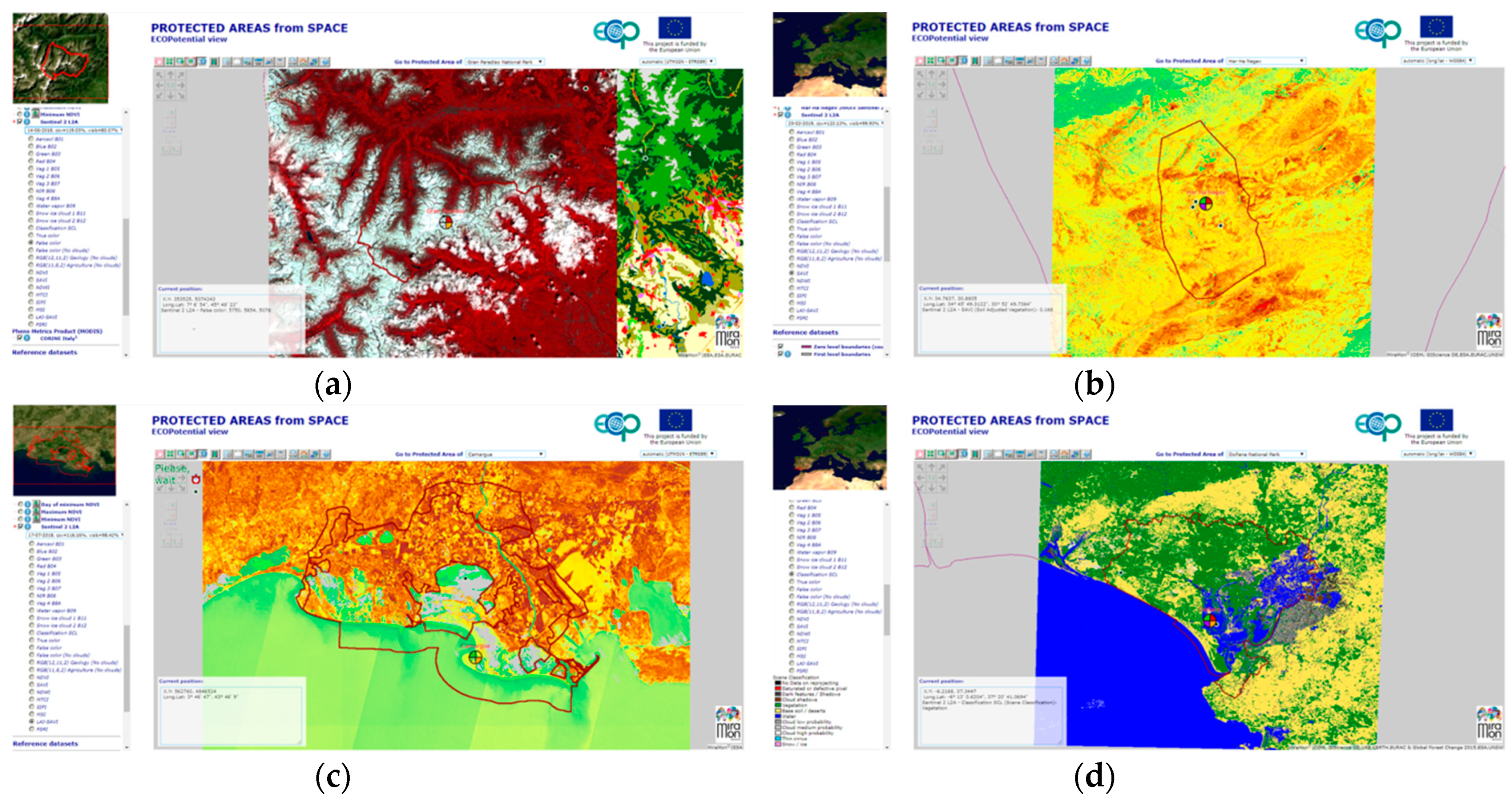
Figure 10 shows the distribution of the protected areas and the ones included in the data cube. We decided to index all granules for all protected areas in the data cube as a single product. Due to the extension of the area, the ingestion process needed to be separated in different products, one for each UTM fuses (see
Table 1). When the WMS service is created, each protected area has its own layer name. In numbers this resulted in one year of Sentinel 2 Level 2A data; 2553 granules consisting in 199360 jp2 files requiring 4.16 TB and resulting in 1693 daily scenes (considering all protected areas). The
Figure 11 shows a few examples of the use of Sentinel 2 images from the ECOPotencial Data Cube in the Protected Areas from Space map browser.
After demonstrating that the approach could be easily generalized to other regions of the world we decided to publish the Python scripts that we used in a GitHub repository (
https://github.com/joanma747/CatalanDataCube) acknowledging that they are actually deeply inspired and based on previous routines exposed by the ODC developer team.
5.2. Does the Presented Open Data Cube Approach Scale up?
The data cube approach adopted by the CDC, represents an important step towards in the simplification of the data preparation and data access of Earth Observation using inexpensive hardware. However, for the approach to be agile it requires to use local storage in the form of random access storages: Hard drives. Mass market hard drives are limited to 12 TB and dual Intel Xeon main boards support only 6 SATA drives. This type of hardware limits the capacity to a maximum of 72 TB. The use of extension boards adds a maximum of 12 SAS drives (depending on the hardware) thus extending the storage capacity to 144 + 72 = 216 TB. Assuming (a) a conservative scenario where the storage capacity is not going to increase significantly in the next years, (b) the amount of Sentinel 2 data will remain constant in the 2 TB used by the indexed and ingested data from March 2018 to March 2019 presented before (c) we might store up to five similar products (including other platforms such as Landsat and other Sentinel as well as some derived products) and (d) an annual increase of the data availability that will grow by a factor of about 1.7 every year (as shown by Reference [
20] for the last 4 years), this approach can be supported by a single similar computer for about 10 years for a region of the same size than Catalonia and in a similar latitude. For a territory 10 times bigger, the approach can only be applied for 5 years.
Of course, there are other options for digital storage but they will require a much bigger investment. This might sound discouraging but it actually means that the ODC is the right solution for today data volume and it is enough for the big data research questions that we are facing now. In the future, other solutions will be needed, such as the possibility to move the whole data cube to the cloud.
The approach to the time series analytics in the client side presented here also has its limitations. In ten years time, a time series of about 130 time frames will become 1300 frames requiring 10 times more memory space for storing the binary arrays. Fortunately, in the 64 bit systems used today, there is almost no logical direction memory limit and the amount of physical memory is regularly increasing so we do not expect to reach any ceiling in the next decade. Note that the quantity of memory needed to handle a time series in the client does not depend on the size of the territory studied or on the scale used, because the client requests only an invariable number of screen pixels to the server.
Another factor to take into account is the amount of time required to transmit a time series from the server to the client. Currently, it takes about 3 m to complete the transference. Assuming that generation and transmission times remain constant, a 10 year long time series might require an unacceptable amount of time. Time series is now being requested as a sequence of independent WMS GetMap requests, one for each time frame. The same WMS standard can be used to request a multidimensional data cube specifying a time interval. By allowing the server to generate the complete multidimensional data, a new more compact multidimensional data structure might be applied that might take advantage of the redundancy in the time series resulting in a considerable decrease in the transmission time.
For the determination of statistical images, an extrapolation of what is happening today with a single year will result in unacceptable computational times of several minutes. The solution for this is a combination of better memory structures with a code optimization. JavaScript code is interpreted by the browser during the runtime, thus becoming very sensible to inefficiencies in certain costly operations that once detected are easily avoidable. The suggested memory structures should favor the easy extraction of the time series for a single point in space keeping, the extraction of a single time frame reasonable efficient.
5.3. Can the Screen Based Analytics Be Translated into a Full Resolution Analytics?
The main difference between the original SatCat and the new web portal is the ability of the latter to work with the actual values derived from the satellite measurements instead of being limited to show pictorial representations. This allows for some data analytics and pixel-to-pixel and local neighbour processing in the client side. The processing is done at screen resolution and happens each time that the user pans or zooms, creating the illusion of a pre existing result. Some analytics (such as filtering) is propagated to the entire time series giving the impression that the process is spread to the time dimension. The browser is able to save the status of the session and when the same page is loaded again, the illusion continues. However, the user might examine the results and become convinced that the tested processing is satisfactory and that he wants to execute it at full resolution and save it as a new product. We are considering adding this functionality to the CDC and we are evaluating three options. The first option consists of adding a piece of software that transforms the JavaScript operations into Python routines, which the ODC could execute directly in the server side. This solution has the advantage that the new results could be immediately exposed as new products in the data cube, but has the disadvantage that the hardware of the CDC needs to execute the processing. We have already described that the whole idea was to demonstrate that a modest hardware could be used for the data cube so this solution will not scale up to many users. Another approach could be to implement a OGC WCS access into the data cube. In this case, users could use the WCS GetCoverage operation to download the information and execute the processing in another facility or in their own computers. This approach might require too much time and bandwidth to complete the transfer. A final solution could be to implement a WCPS in the CDC. WCPS [
21] provides a collection of operations and a query language to remotely execute analytical processes. The WCPS standard is agnostic on where the processing is done. The WCPS implementation (such as Rasdaman) could use the data coming from the CDC and redirect and distribute the processing among the available processing facilities providing a more scalable solution.
6. Conclusions
The ODC has been advertised as a platform allowing nations to organize and process remote sensing products provided by the main Earth Observation satellites. The amount of data that some of these products generate requires automatic solutions for simplifying the data download and use. This paper demonstrates that the approach is equally useful for a sub-national region such as Catalonia or for smaller natural regions that require information for their management, such as the protected area network of the ECOPotential project. Even if ODC helps in organizing the data, it still requires knowledge on the ODC API and Python programming, limiting the accessibility of the data to expert users. The paper proposes the addition of another layer of software consisting of a web map browser that combines the interoperability of the state of the art OGC WMS standard with the new possibilities offered by the HTML5 to present data in a way that everybody can explore and understand without any need of programming skills. In addition, it demonstrates a promising strategy based on multidimensional binary arrays allowing for some time series analytics that the current web browser can execute and that will be extended in the future. Currently, animations, temporal profiles, x/t images, and images representing mean values and variations can be generated by the user in the map browser without any server intervention.
The paper proposes the use of modest off-the-shelf computer hardware and concludes that the current approach can reach some limits in 10 years time but still can offer a solution to analyze the state and the evolution of the planet valid up to the next decade. The paper also analyzes the real availability of Sentinel 2 data over Catalonia showing huge variations in the area due to the distribution of the Sentinel 2 paths and swath overlaps, but also the effect of clouds, concluding that, in 2018, some South and central regions of Catalonia get more than one useful image per week, while in others situated in the Pyrenees and Eastern areas, only an average of one or two images per month were useful.
This work is inspired by the original SatCat Landsat service for the Catalonia region (with coverage starting in the 1972) and extends and complements it with a new useful service that is maintained automatically, incorporates Sentinel 2 data, and provides time series analysis.


 ) where the set of time slices of the area defined in the main window will be requested, visualized, and analyzed. For each time slice, the components are downloaded, saved in memory and rendered in a HTML independent division (HTML DIV) that contains a canvas. Creating the animation effect is as simple as hiding all divisions and making visible one of them in sequence (see Figure 3e). Modern browsers are fast in doing this kind of hiding operations allowing for speeds higher than 10 frames per second, thus resulting in a quite convincing video effect.


