Abstract
To achieve the optimal performance of an object to be heat treated, it is necessary to know the value of the Heat Transfer Coefficient (HTC) describing the amount of heat exchange between the work piece and the cooling medium. The prediction of the HTC is a typical Inverse Heat Transfer Problem (IHCP), which cannot be solved by direct numerical methods. Numerous techniques are used to solve the IHCP based on heuristic search algorithms having very high computational demand. As another approach, it would be possible to use machine-learning methods for the same purpose, which are capable of giving prompt estimations about the main characteristics of the HTC function. As known, a key requirement for all successful machine-learning projects is the availability of high quality training data. In this case, the amount of real-world measurements is far from satisfactory because of the high cost of these tests. As an alternative, it is possible to generate the necessary databases using simulations. This paper presents a novel model for random HTC function generation based on control points and additional parameters defining the shape of curve segments. As an additional step, a GPU accelerated finite-element method was used to simulate the cooling process resulting in the required temporary data records. These datasets make it possible for researchers to develop and test their IHCP solver algorithms.
Dataset: DOI:10.5281/zenodo.3237781.
Dataset License: CC-BY
1. Summary
Heat treatment operations are used to change the material properties of components. The controlled input or extraction of heat is essential during the whole process. Quenching processes are typically operated in different liquid or gaseous media to achieve the desired material properties by following the adequate heat transfer rates. A commonly used industrial hardening procedure is immersion quenching. In this process, the work pieces are heated to the desired temperature and then immersed in the liquid quenching medium.
The heat transfer phenomena occurring during the quenching process may pass three different boiling regimes [1]. In the first stage, the component is surrounded by a vapor film, which insulates the work piece. The heat transfer is moderated in this stage and takes place by radiation and conduction through the vapor film.
In the second stage, the surface partially gets in contact with the coolant when the temperature reaches the Leidenfrost point and nucleate boiling occurs with the fastest cooling rate during the whole heat transfer process. Then, the surface cools down below the boiling point (or range) and only pure convection occurs. In this stage, the heat transfer mainly is controlled by the quenchant’s specific heat and thermal conductivity, and temperature differences between the surface and the fluid combined with fluid flow.
To achieve the desired mechanical properties of the components, it is necessary to know the characteristics of the Heat Transfer Coefficient (HTC) describing the heat exchange between the work piece and the surrounding cooling medium. The prediction of the HTC is a typical ill-posed task, which cannot be solved by direct numerical methods. In recent years, this Inverse Heat Transfer Problem (IHCP) has been studied extensively [2,3,4,5,6], presenting various heuristic solutions based on Genetic Algorithms (GA) [7,8] or Particle Swarm Optimization (PSO) [7,9]. There are also promising results in the development of the sparse representation for ill-posed problems [10].
In the case of these population based methods, each instance (chromosome in GA/particle in PSO) represents a HTC function candidate, and its fitness is calculated by the squared difference between some real-world measurements and the results of the generated temperature data using the HTC values encoded in the instances. There are promising results; however, these processes usually need thousands of instances and iterations. The number of fitness function evaluations (which is the most computationally intensive part of the search) is the multiplication of the population size and the iteration count; for this reason, these methods are usually very time-consuming. A whole search takes hours or days and (as is common for heuristic methods) hundreds of executions are necessary to have stable results.
Artificial Neural Networks (ANN) were motivated by the already existing biological structures of the brain [11], having powerful capabilities for tasks such as learning, pattern matching and adaptation. As the real biological brain, the basic construction units of ANNs are artificial neurons connected by weighted edges. In the simplest architecture, the input and output neurons are connected through one or more layers of hidden ones. In the case of densely connected ANNs, all neurons of a given hidden or output layer are connected to all neurons of the previous layer. There are several advanced architectures (convolutional neural networks, etc.) and the choice between these needs a lot of research and experiments. In the case of feed-forward neural networks, the information moves in only one direction: from the input neurons to the output nodes through the hidden ones. If we know the appropriate weight values for edges, the feed-forward operation of the ANN is given by Equation (1).
where X is the vector of the input data; W is the matrix of edge weights; b is the vector of bias constant values; f is an activation function; and Y is the vector containing the prediction of the network.
X and f are known but the values of the W and b variables needs some preprocessing. There are various techniques to determine the values of these weights, one of the most widely used being the back-propagation algorithm. It is a supervised training method, which means that it learns from valid input and output data pairs, called the training data. The back-propagation algorithm starts with random W and b values, feeds the network with the input data and measures the difference between the prediction of the network (Y) and the known valid output (). After that, the error is propagated back to the previous layers recursively and the weights of edges are adjusted according to this. This process is repeated until the loss (difference between the desired and actual output) is satisfactory. After this learning process, it is possible to save the state of the ANN, and it is able to do predictions for new inputs.
ANNs have already been used by researchers of the field, and there are superior results in reducing the material parameters for selected material functions [12]. Our presented feed-forward network is applicable to do the reverse engineering task of the IHCP. Feeding the measured temperature records to the network as an input, it may be able to predict the main characteristics of the HTC. Both the temperature and the HTC series are based on time, therefore the input and the output of the network should be quite large. Nowadays, the availability of modern GPUs makes it possible to design quite large dense networks, and train them in a tolerable time.
Modern GPUs can be considered as general purpose architectures with a large number of simple processing cores. Nowadays, these devices are the key factors to solving highly computing-intensive tasks. GPU hardware has two particular strengths: high number of cores and memory bandwidth. This new programming model forces the programmer to divide the problem into a block of threads and running thousands of these. A problem is suitable for GPU acceleration only if it is able to adapt to these requirements and utilize the benefits. Focusing on the topic of this paper, there are two areas where it is possible to take advantage of these: running complex simulations with Finite-Element Method (FEM) and training ANNs.
Beyond the computational demands, the other constraint for the efficient training process is the availability of enough training data. To train a network with hundreds/thousands of hidden neurons, millions of training data pairs are required. Although there are several real-world measurements, the number of them is far from satisfactory. The only way to have enough data is through the generation of corresponding HTC/temperature series pairs. This also raises some problems:
- It is necessary to construct a model for building potential HTC series.
- The temperature history for a given HTC can be generated by a cooling simulation process, which is very time consuming in the case of millions of inputs.
2. Data Description
The dataset includes more than 1 million records of Heat Transfer Coefficient and corresponding Temperature value pairs. HTC is given by as a function of temperature; the temporal history is given by as the function of time. HTC values are stored in the file named “xxx_htc_header.bin” and “xxx_htc_data.bin”, while temperature values are stored in the file named “xxx_temp_data.bin”.
2.1. Heat Transfer Coefficient File
The format of the HTC header file is given by Table 1.

Table 1.
Description of on record in the HTC header file.
The format of the HTC data file is given by Table 2.
Table 2.
Description of one record in the HTC data file.
Additional notes concerning these files:
- All values are encoded as floats, even though some of them are integers (number of control points).
- The number of control points is always 5.
- The value of is 10 °C. Therefore, the number of HTC values is 86, according to temperatures 0 °C, 10 °C, 20 °C, …, 850 °C.
- The size of one header record is 64 bytes.
- The size of one data record is 344 bytes.
According to the common patterns of neural network training, the database contains three file pairs:
- Training set: The training database, containing 1,000,000 record pairs
- –
- “train_htc_header.bin”: The header part of the training dataset ( megabytes)
- –
- “train_htc_data.bin”: The data part of the training dataset ( megabytes)
- Validation set: The validation database, containing 100,000 record pairs
- –
- “valid_htc_header.bin”: The header part of the validation dataset ( megabytes)
- –
- “valid_htc_data.bin”: The data part of the validation dataset ( megabytes)
- Test set: The test database, containing 100,000 record pairs
- –
- “test_htc_header.bin”: The header part of the test dataset ( megabytes)
- –
- “test_htc_data.bin”: The data part of the test dataset ( megabytes)
2.2. Temperature File
The format of the Temperature file is given by Table 3. As visible, it simply contains the temperature records for a given simulation using s resolution. As it is a cooling process, it starts with 850 °C and converges to room temperature.
Table 3.
Description of one record in the temperature file.
Additional notes about these files:
- The value of is s. Therefore, the number of temperature values is 121, according to time s, 1 s, …, 60 s.
- The size of one data record is 480 bytes.
According to the common patterns of neural network training, the database contains three files:
- Training set: The training database, containing 1,000,000 records
- –
- “train_temp_data.bin”: The temperature data of the training dataset
- Validation set: The validation database, containing 100,000 records
- –
- “valid_temp_data.bin”: The temperature data of the validation dataset
- Test set: The test database, containing 100,000 records
- –
- “test_temp_data.bin”: The temperature data of the test dataset
3. Methods
3.1. Model for HTC Generation
Considering the one-dimensional IHCP, the HTC is a one-dimensional function of temperature given between 0 °C and 850 °C.
The generation of HTC series is based on control points. Each HTC function is given by N control points . In the case of one-peak functions, it is enough to use three control points (); in the case of two-peak functions, the number of required control points is 5 (). Each control point has a temperature () and a HTC () coordinate, according to the constraints given by Equations (2)–(4).
Based on 300 real world measurements, Table 4 contains the additional value constraints.
Table 4.
Limits for control points (N=5).
Figure 1 shows an example of how the control points describe the breakpoints of the function. It is not visible in the figure, but there are two (where = 0 °C and ) and (where = 850 °C and ) virtual control points to handle the first and last section of the function.
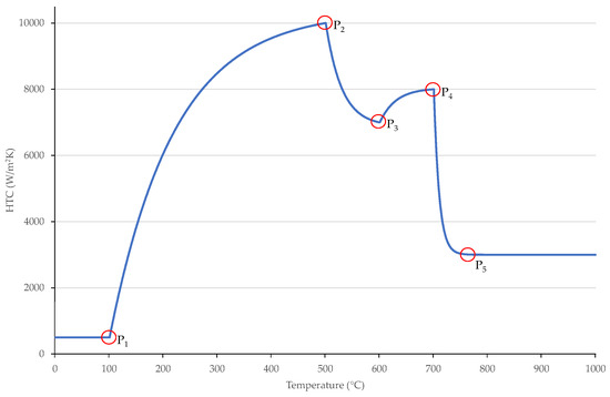
Figure 1.
control points of an example HTC function.
The shape of the curve of each segment between control points is controlled by a single floating point number (), according to Equation (5).
The HTC value for a given T temperature between control points and is given by the following equations:
where is a scaling factor (usually 7); is the control point before T; is the control point after T; is the ith curve shape attribute; T is the temperature; and is the HTC value for the given temperature.
Figure 2 shows the effect of different parameters. The selection leads to a division by zero error. In this special case, the points of the linear curve are simply calculated by Equation (10).
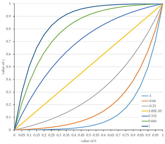
Figure 2.
Calculated values by for different parameters.
Using the presented model, it is possible to randomly generate HTC series. Using the limits of Table 4 and random values between and for all control points, the shape of the HTC function is specified by the given Equations (9) and (10). For further processing, we store the calculated values of the HTC function for given temperature values, from 0 °C to 850 °C using 10 °C steps.
3.2. Temperature History Generation
To solve the IHCP, the temperature history for given HTC series is also necessary. The presented dataset is composed of information representing the quenching process from 850 °C to room temperature of a cylindrical bar (diameter: 20 mm; and length: 60 mm) produced from Inconel 600 alloy. The physical properties of Inconel 600 alloy are summarized in Table 5 and Table 6. Its density is 8420 kg/m. The probe was equipped with one thermocouple located 30 mm from the bottom at the centerline of the cylinder. Due to the position of the thermocouple, only radial exchange was assumed, therefore a 1D axis-symmetrical Heat Transfer model was applied for the calculations [13]. The HTC was considered as a function of the surface temperature. The cooling curves at the location of the thermocouple were obtained by using HTC(T) function as input for the heat transfer model.
Table 5.
The heat conductivity of ISO 9950 alloy.
Table 6.
The specific heat of ISO 9950 alloy.
The explicit finite difference method (FDM) presented by Smith was used to simulate the heat movement. In the case of one-dimensional heat transfer simulation, it is necessary to solve the following equations:
where is the temperature of the ith node of the finite element matrix at time t; is the thermal diffusivity (Equation (14)); k is the thermal conductivity; is the specific heat capacity; is the density of the material; is the heat transfer coefficient; N is the number of points; and is the temperature of the cooling medium.
The problem domain was discretized to approximate the solution to the given problem. It was done by dividing the domain into a uniform grid, and the cross section of the object was substituted with an N-sized vector.
Using the finite difference method, the heat transfer between the given areas was calculated using one time step. To ensure accuracy, the sufficiently small time interval () selection is essential ( s was used). The simulation needed to run a cycle of the calculations mentioned above to generate the temperature values for each time step. The above-mentioned method is well-suited for several situations; however, the calculation demand is quite high. We had to calculate the given formulas for all nodes for all given time steps. In the case of and 1 min simulation time, the number of calculations was .
In normal circumstances, this is acceptable, because an average CPU can calculate the results in some seconds. In this case, the goal is to generate a database from these; therefore, it is necessary to run millions of simulations, which is very time consuming. Because it is a well parallelizable task, the authors have already developed a novel GPU based acceleration for this process.
The main idea behind GPGPU (General-Purpose Computing on Graphical Processing Units) is to use the architecture of a massive number of processing units to solve computationally intense cases. There are already several successful research projects in this field [14,15,16]. The novel parallel algorithm implemented by the authors is based on several optimization steps: launching multiple threads on all multiprocessors, storing data in fast on-chip memory, eliminating warp divergence and memory transfer latency, and using the host and device together [17,18]. It makes it possible to run all necessary simulations in a tolerable time.
Figure 3 shows some examples for these generated HTC functions and temperature records.
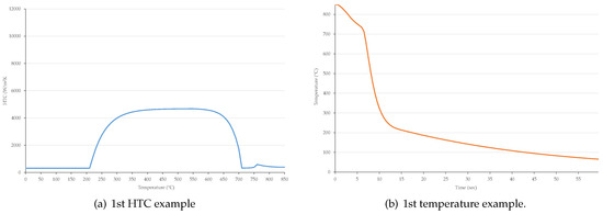
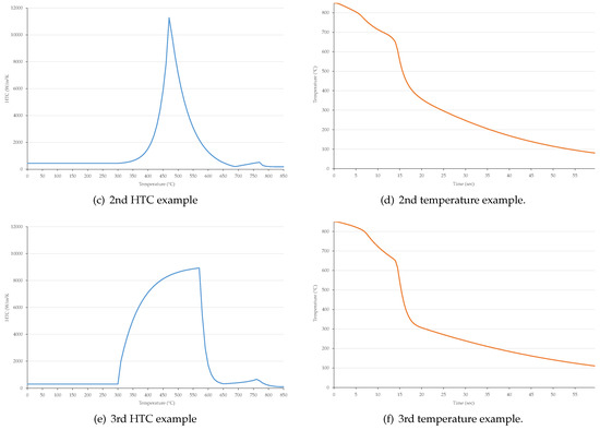
Figure 3.
Examples for generated HTC functions and the corresponding simulated temporal history.
4. Usage Notes
This paper presents a database containing HTC functions and the corresponding temperature records. The authors designed a novel method for generating valid HTC functions based on several real-world measurements. The corresponding temperature function is the result of a simulation process, which was accelerated by graphics cards, due to high computational demands. This database makes it possible to design novel methods to solve the IHCP. In the case of machine-learning-based approaches, the proposed database is directly usable for training, testing and validation of solutions.
The authors presented several methods to determine the HTC based on temperature data. These are mostly based on time consuming, heuristic searches (genetic algorithms [19,20], particle swarm optimization [21,22,23], fireworks [24], etc.). As an alternative, based on a similar generated database, it was possible to develop another approach based on Universal Function Approximator networks. The authors designed a simple feed-forward dense ANN to solve the IHCP [25]. This model contains 120 input neurons and 101 output neurons. The activation function was the sigmoid function and the loss function was designed as the mean squared error between the prediction and the training output. The network used AdamOptimizer with learning rate 0.01. The authors ran several tests with various hidden layer sizes, and the best results was given by the layer of 50 neurons. This ANN was able to estimate the HTC based on the temporal data series (Figure 4).
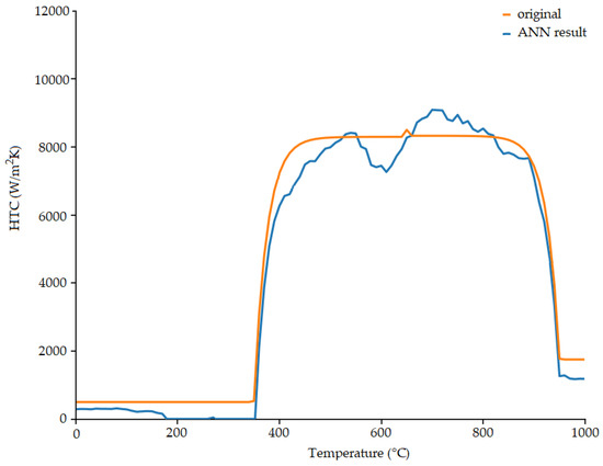
Figure 4.
Sample result given by a simple feed-forward network trained on a similar database. The orange line is the original generated HTC. The blue line is the predicted HTC given by the neural network based on the temperature curve. The network was trained by HTC-temperature function pairs [25].
However, it is evident that the accuracy of this method is not satisfactory. It needs further development to find the appropriate network architecture, the optimal number of nodes, etc. It is a time consuming process, because training a network, with such a large amount of data, would take multiple weeks, and this process is necessary to test each potential architecture. This was the reason the authors decided to open the proposed database, for all of the researchers in this field.
Author Contributions
Conceptualization, S.S. and I.F.; Methodology, S.S. and I.F.; and Writing—Review and Editing, S.S. and I.F.
Funding
This research received no external funding.
Acknowledgments
Sándor Szénási would like to thank EPAM Systems for their support.
Conflicts of Interest
The authors declare no conflict of interest. The funders had no role in the design of the study; in the collection, analyses, or interpretation of data; in the writing of the manuscript, or in the decision to publish the results.
References
- Mackenzie, D.S. Advances in Quenching A Discussion of Present and Future Technologies. In Proceedings of the 22nd Heat Treating Society Conference and the 2nd International Suface Engineering Congress, Indianapolis, Indiana, 12–17 September 2003; pp. 21–28. [Google Scholar]
- Alifanov, O.M. Inverse Heat Transfer Problems; Springer: Berlin/Heidelberg, Germany, 1994. [Google Scholar]
- Nelder, J.A.; Mead, R. A simplex method for function minimization. Comput. J. 1965, 7, 308–313. [Google Scholar] [CrossRef]
- Lagarias, J.C.; Reeds, J.A.; Wright, M.H.; Wright, P.E. Convergence Properties of the Nelder–Mead Simplex Method in Low Dimensions. SIAM J. Optim. 1998, 9, 112–147. [Google Scholar] [CrossRef]
- Das, R. A simplex search method for a conductive–convective fin with variable conductivity. Int. J. Heat Mass Transf. 2011, 54, 5001–5009. [Google Scholar] [CrossRef]
- Nelles, O. Nonlinear System Identification; Springer: Berlin/Heidelberg, Germany, 2001. [Google Scholar]
- Colaço, M.J.; Orlande, H.R.B.; Dulikravich, G.S. Inverse and optimization problems in heat transfer. J. Braz. Soc. Mech. Sci. Eng. 2006, 28, 1–24. [Google Scholar] [CrossRef]
- Özisik, M.N.; Orlande, H.R.B. Inverse Heat Transfer: Fundamentals and Applications; Taylor & Francis: Didcot, UK, 2000. [Google Scholar]
- Vakili, S.; Gadala, M.S. Effectiveness and Efficiency of Particle Swarm Optimization Technique in Inverse Heat Conduction Analysis. Numer. Heat Transf. Part B-Fundam. 2009, 56, 119–141. [Google Scholar] [CrossRef]
- Qiao, B.; Liu, J.; Liu, J.; Yang, Z.; Chen, X. An enhanced sparse regularization method for impact force identification. Mech. Syst. Signal Process. 2019, 126, 341–367. [Google Scholar] [CrossRef]
- Guan, J.S.; Lin, L.Y.; Ji, G.L.; Lin, C.M.; Le, T.L.; Rudas, I.J. Breast tumor computer-aided diagnosis using self-validating cerebellar model neural networks. Acta Polytech. Hung. 2016, 13, 39–52. [Google Scholar] [CrossRef]
- Sumelka, W.; Łodygowski, T. Reduction of the number of material parameters by ANN approximation. Comput. Mech. 2013, 52, 287–300. [Google Scholar] [CrossRef][Green Version]
- Felde, I.; Szénási, S. Estimation of temporospatial boundary conditions using a particle swarm optimisation technique. Int. J. Microstruct. Mater. Prop. 2016, 11, 288–300. [Google Scholar] [CrossRef]
- Zuo, H.; Yang, Z.B.; Sun, Y.; Xu, C.B.; Chen, X.F. Wave propagation of laminated composite plates via GPU-based wavelet finite element method. Sci. China Technol. Sci. 2017, 60, 832–843. [Google Scholar] [CrossRef]
- Aciu, R.M.; Ciocarlie, H. Runtime Translation of the Java Bytecode to OpenCL and GPU Execution of the Resulted Code. Acta Polytech. Hung. 2016, 13, 25–44. [Google Scholar]
- Cotronis, Y.; Konstantinidis, E.; Louka, M.A.; Missirlis, N.M. A comparison of CPU and GPU implementations for solving the Convection Diffusion equation using the local Modified SOR method. Parallel Comput. 2014, 40, 173–185. [Google Scholar] [CrossRef]
- Szénási, S. Solving the Inverse Heat Conduction Problem using NVLink capable Power architecture. PeerJ Comput. Sci. 2017, 3, 1–20. [Google Scholar] [CrossRef]
- Szénási, S.; Felde, I. Using Multiple Graphics Accelerators to Solve the Two-dimensional Inverse Heat Conduction Problem. Comput. Methods Appl. Mech. Eng. 2018, 336, 286–303. [Google Scholar] [CrossRef]
- Szénási, S.; Felde, I. Configuring Genetic Algorithm to Solve the Inverse Heat Conduction Problem. In Proceedings of the 5th International Symposium on Applied Machine Intelligence and Informatics (SAMI2017), Herl’any, Slovakia, 26–28 January 2017; pp. 387–391. [Google Scholar]
- Szénási, S.; Felde, I. Configuring Genetic Algorithm to Solve the Inverse Heat Conduction Problem. Acta Polytech. Hung. 2017, 14, 133–152. [Google Scholar] [CrossRef]
- Felde, I.; Fried, Z.; Szénási, S. Solution of 2-D Inverse Heat Conduction Problem with Graphic Accelerator. Mater. Perform. Charact. 2017, 6, 882–893. [Google Scholar] [CrossRef]
- Szénási, S.; Felde, I. Modified Particle Swarm Optimization Method to Solve One-dimensional IHCP. In Proceedings of the 16th IEEE International Symposium on Computational Intelligence and Informatics (CINTI2015), Budapest, Hungary, 19–21 November 2015; pp. 85–88. [Google Scholar] [CrossRef]
- Szénási, S.; Felde, I.; Kovács, I. Solving One-dimensional IHCP with Particle Swarm Optimization using Graphics Accelerators. In Proceedings of the 10th Jubilee IEEE International Symposium on Applied Computational Intelligence and Informatics (SACI2015), Timisoara, Romania, 21–23 May 2015; pp. 365–369. [Google Scholar]
- Fried, Z.; Pintér, G.; Szénási, S.; Felde, I.; Szél, K.; Sáfár, A.; Sousa, R.; Deus, A. On the Nature-Inspired Algorithms Applied to Characterize Heat Transfer Coefficients. In Proceedings of the Thermal Processing in Motion 2018, Spartanburg, SC, USA, 5–7 June 2018; pp. 47–51. [Google Scholar]
- Szénási, S.; Felde, I. Estimating the Heat Transfer Coefficient using Universal Function Approximator Neural Network. In Proceedings of the 12th International Symposium on Applied Computational Intelligence and Informatics (SACI2018), Timisoara, Romania, 17–19 May 2018; pp. 401–404. [Google Scholar] [CrossRef]


© 2019 by the authors. Licensee MDPI, Basel, Switzerland. This article is an open access article distributed under the terms and conditions of the Creative Commons Attribution (CC BY) license (http://creativecommons.org/licenses/by/4.0/).