A Novel Ensemble Neuro-Fuzzy Model for Financial Time Series Forecasting

Abstract

Neuro-fuzzy models have a proven record of successful application in finance. Forecasting future values is a crucial element of successful decision making in trading. In this paper, a novel ensemble neuro-fuzzy model is proposed to overcome limitations and improve the previously successfully applied a five-layer multidimensional Gaussian neuro-fuzzy model and its learning. The proposed solution allows skipping the error-prone hyperparameters selection process and shows better accuracy results in real life financial data.

1. Introduction

Time series forecasting is an important practical problem and a challenge for Artificial Intelligence systems. Financial time series have a particular importance, but they also show an extremely complex nonlinear dynamic behavior, which makes them hard to predict.

Classical statistical methods dominate the field of financial data and have a long history of development. Nevertheless, in many cases they have significant limitations like restrictions on datasets, require complex data preprocessing and additional statistical tests.

Artificial intelligence models and methods have been competing classical statistical approaches in many domains including financial forecasting and analysis. Neuro-fuzzy systems naturally inherit strengths of artificial neural networks and fuzzy inference systems, and have been successfully applied to a variety of problems including forecasting. Rajab and Sharma [1] made a comprehensive review of the application of neuro-fuzzy systems in business.

Historically, ANFIS—Adaptive Network Fuzzy Inference System, proposed by Jang [2], was the first successfully applied neuro-fuzzy model and most of the later works have been based on it.

Examples of successfully applied ANFIS-derived models for stock market prediction are the neuro-fuzzy model with a modification of the Levenberg–Marquardt learning algorithm for Dhaka Stock Exchange day closing price prediction [3] and an ANFIS model based on an indirect approach and tested on Tehran Stock Exchange Indexes [4].

Rajab and Sharma [5] proposed an interpretable neuro-fuzzy approach to stock price forecasting applied to various exchange series.

García et al. [6] applied a hybrid fuzzy neural network to predict price direction in the stock market index, which consists of the 30 major German companies.

In order to improve results by further hybridization, neuro-fuzzy forecasting models in finance were combined with evolutionary computing as, e.g., in Hadavandi et al [7]. Chiu and Chen [8] and Gonzalez et al. [9] described models which use support vector machines (SVM) together with fuzzy models and genetic algorithms. Another effective approach is to exploit the representative capabilities of wavelets (for instance, Bodyanskiy et al. [10], Chandar [11]) and recurrent connections as in Parida et al. [12] and Atsalakis and Valavanis [13]. Cai et al. [14] used ant colony optimization. Some optimization techniques were applied to Type-2 models [15,16,17]. All such models benefit from combining the strengths of different approaches but may suffer from the growth of parameters to be tuned.

Neuro-fuzzy models in general require many rules to cover complex nonlinear relations, which is known as the curse of dimensionality. In order to overcome this, Vlasenko et al. [18,19,20] proposed a neuro-fuzzy model for time series forecasting, which exploits multidimensional Gaussians ability to handle nontrivial data dependencies by a relatively small number of computational units. It also displays good computational performance, which is achieved through using a stochastic gradient optimization procedure for tuning consequent layer units and an iterative projective algorithm for tuning their weights.

However, this model also has its limitations, the biggest of which is the necessity to manually choose training hyperparameters and the model sensitivity for this choice. Many different approaches may be applied to hyperparameter tuning, but in general they are greedy for computational resources and may require complex stability analysis. Another issue, despite generally good computational performance, is the inability of the stochastic gradient descent learning procedure to utilize multithreading capabilities of the modern hardware.

The remainder of this paper is organized as follows: Section 2 is devoted to the proposed model architecture and learning, and Section 3 describes the data sets and contains experimental results.

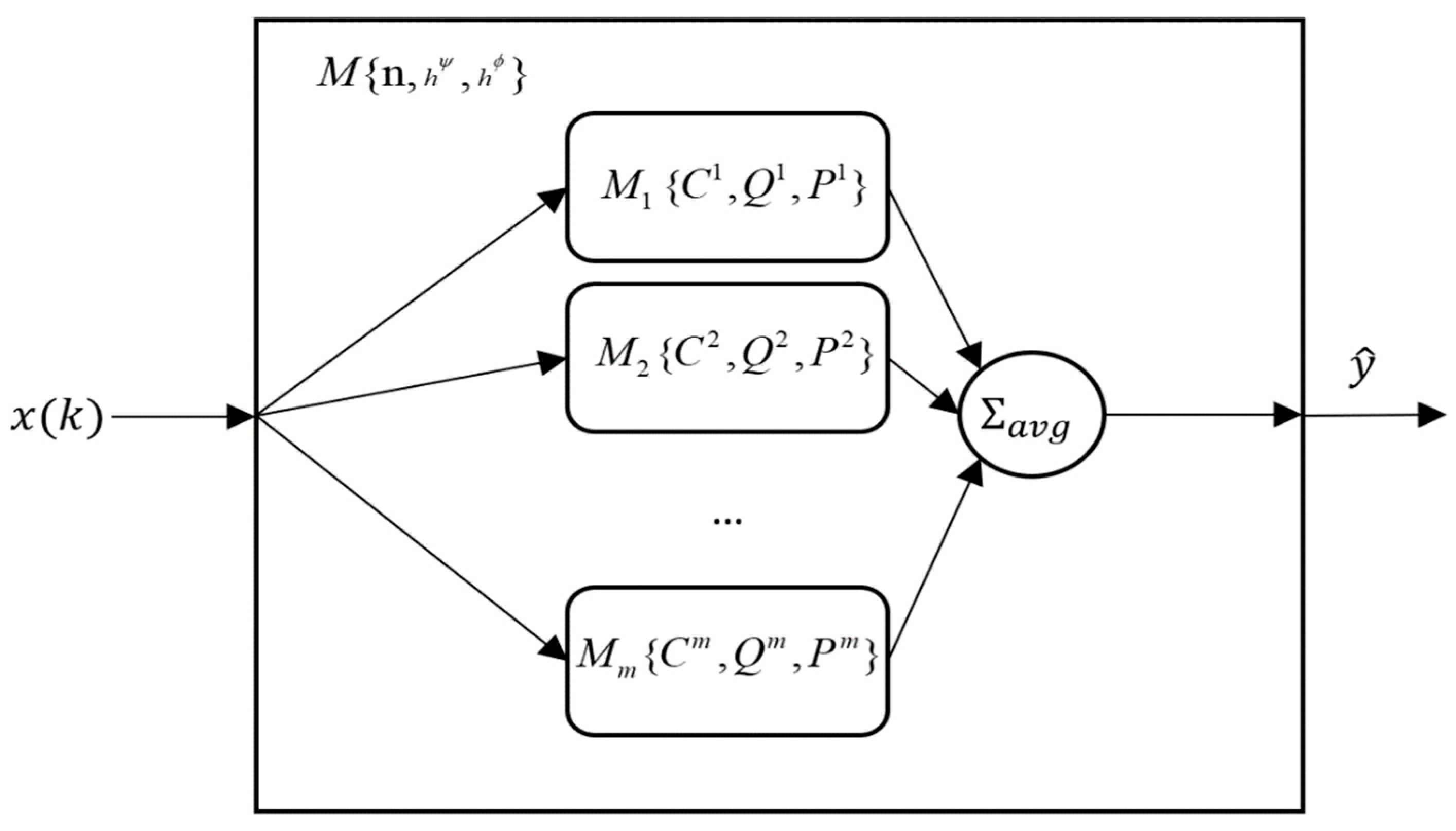
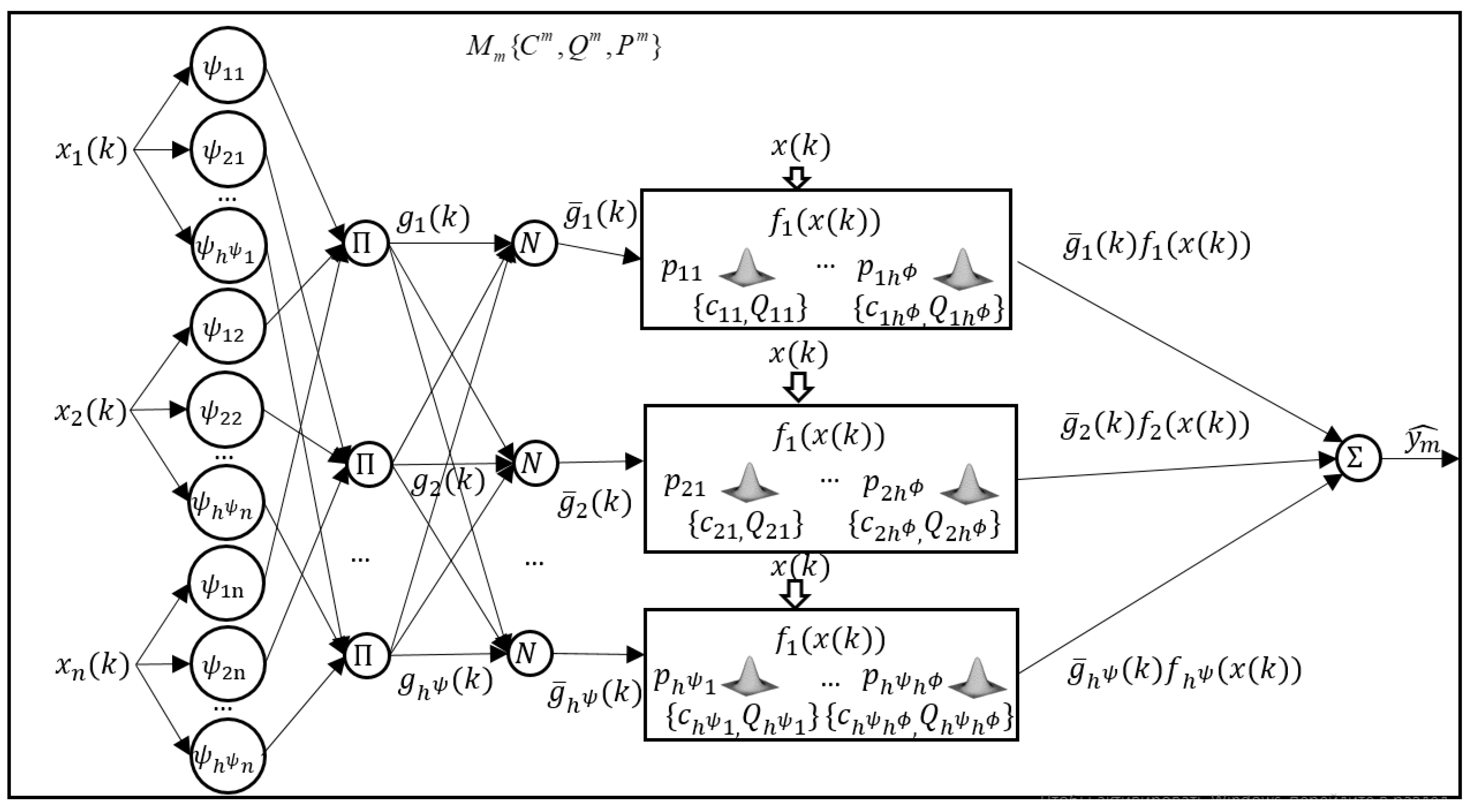
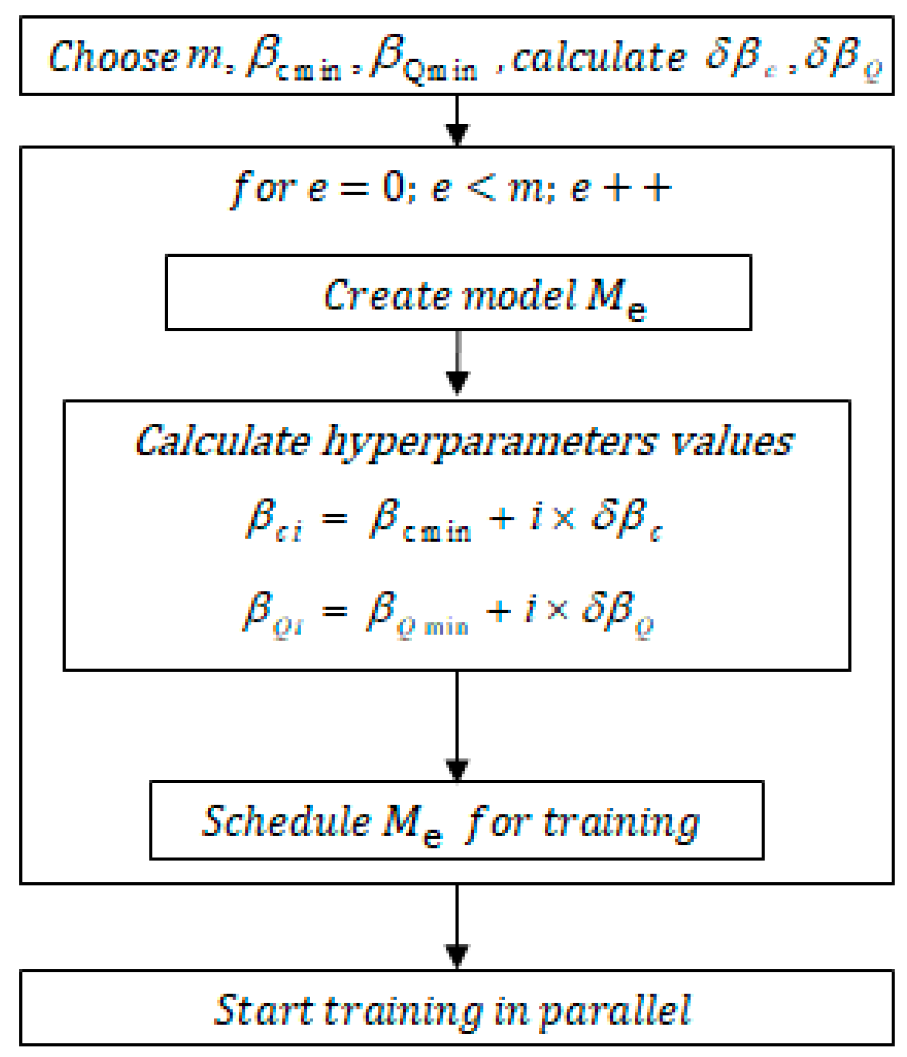
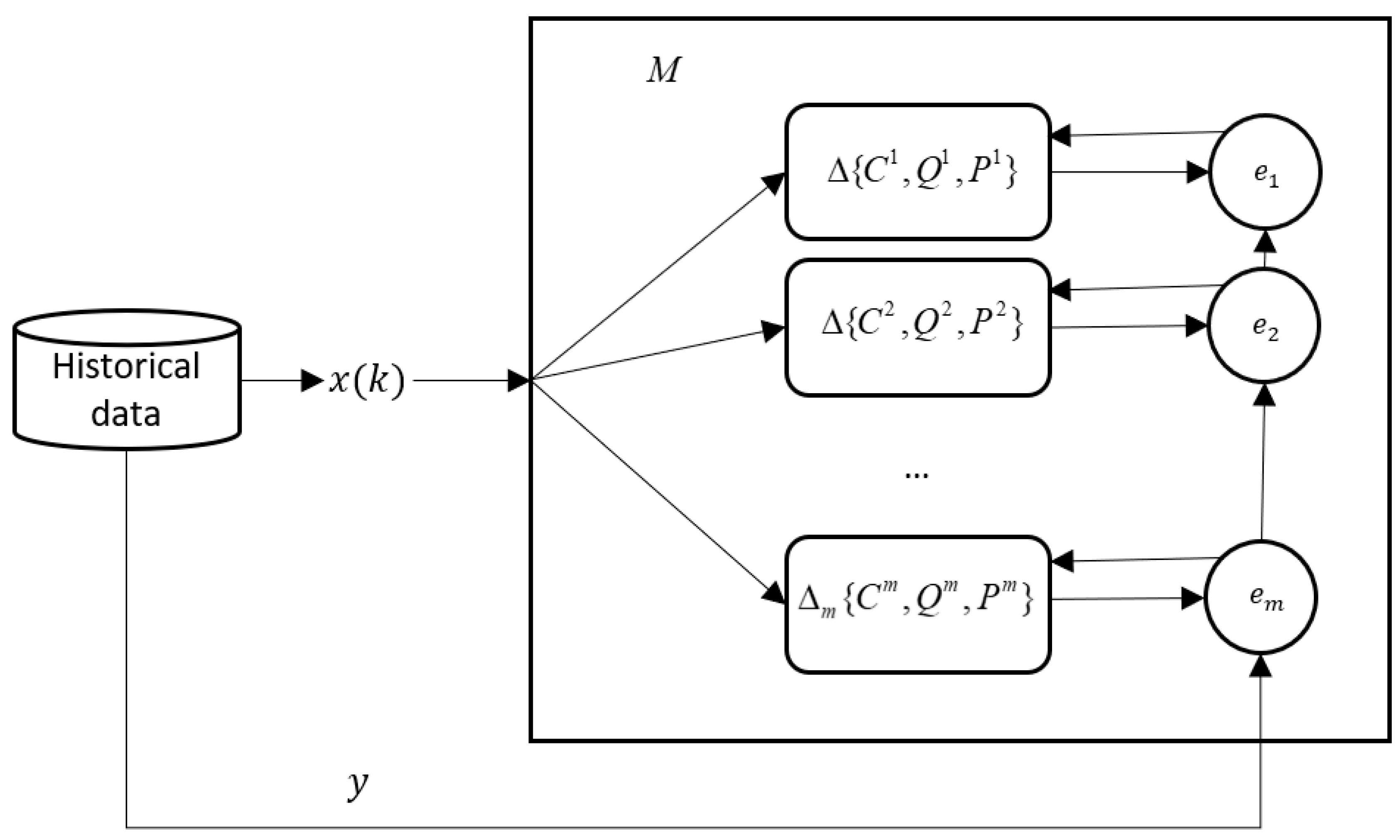
2. Proposed Model and Inference

To solve the aforementioned problems, we propose an ensemble model and an initialization procedure for it. It comprises neuro-fuzzy member models $M_e$. The general architecture presented in Figure 1.

Each input pattern $x\left(k\right)$ is propagated to all models $M_e$. All models have the same structure which is defined by three parameters—the length of input vector $n$, number of antecedent layer functions $h^{\psi }$ and number of consequent node functions $h^{\phi }$ (analogous to a number of polynomial terms in ANFIS). The difference is in the fourth layer parameters $C_{}^e,Q_{}^e,P_{}^e$ which are initialized randomly and then tuned during the learning phase. Matrix $C_{}^e$ represents all vector-centers of the consequent layer functions, matrix $Q_{}^e$—their receptive field matrices (generalization of the function width) and $P_{}^e$—weights matrix.

Then all outputs are sent to the output node ${\mathsf{\Sigma }}_{avg}$, which computes the resulting value $\widehat{y}$ as an average value:

$$\widehat{y}=\frac{{\displaystyle \sum _{e=1}^m{\widehat{y}}_e}}{m}$$

where ${\widehat{y}}_e$ is a member model output, and $m$ is the number of member models. Model averaging is the simplest way to combine different models and achieve better accuracy under the assumption that different models will show partially independent errors, which in turn may lead to better generalization capabilities.

Detailed structure of a five layer member model introduced in [18] is depicted in Figure 2.

Each member model performs an inference by the following formulae:

$${\widehat{y}}_e=p_e{}^T{f}_e\left(x\left(k\right)\right)$$

where $x\left(k\right)={(x_1(k),x_2(k),\dots ,x_n(k))}^T$ is an input vector, $p_e$ is the weights vector (a vector representation of the $P_{}^e$ matrix), and $f_e\left(x\left(k\right)\right)$ is a vector of normalized consequent function values:

$$f_e\left(x\left(k\right)\right)=({\overline{g}}_{e1}{\varphi }_{e11}\left(x\left(k\right)\right)\dots {\overline{g}}_{e{h}^{\psi }}{\varphi }_{e{h}^{\psi }{h}^{\varphi }}\left(x\left(k\right)\right))$$

where $h^{\psi }$ is the number of functions in the first layer and $h^{\phi }$ is the number of multidimensional Gaussians in the fourth layer for each normalized output ${\overline{g}}_{el}$:

$${\overline{g}}_{je}(k)=\frac{g_{je}(k)}{{\displaystyle \sum _{j=1}^{h^{\psi }}{g}_{je}(k)}}=\frac{{\displaystyle \prod _{i=1}^n{\psi }_{jl}e\left(x_i\left(k\right)\right)}}{{\displaystyle \sum _{i=1}^{h^{\psi }}{\displaystyle \prod _{i=1}^n{\psi }_{jl}e\left(x_i\left(k\right)\right)}}}$$

The initialization algorithm is shown in Figure 3. Its goal is to initialize member models before training and set training parameters. Results from [18,20] show that ${\beta }_c$ and ${\beta }_Q$ hyperparameters, which are dumping parameters for optimization of $C_{}^e$ and $Q_{}^e$, respectively, significantly influence accuracy of the model prediction. According to this we create identical member models but set different values for ${\beta }_c$ and ${\beta }_Q$. Centers are placed equidistantly and identity matrices are used as receptive before training. After models are created we can start training them in parallel.

The general training process is depicted in Figure 4. We use historical data as a training set and feed vectors of historical gap values to each model. Then reference value $y\left(k\right)$ is used to calculate error $e_e$ for each local model. Error is then propagated and used to calculate deltas ${\Delta }_m^{}\{C_{}^m,Q_{}^m,P_{}^m\}$ to adjust the model’s free parameters $C_{}^e,Q_{}^e,P_{}^e$.

The training process is focused on multidimensional Gaussian functions of the fourth layer and their weights.

Consequent Gaussians have the following form:

$${\varphi }_{aje}\left(x\left(k\right)\right)=\exp \left(-\frac{{\left(x\left(k\right)-c_{aje}^{\varphi }\right)}^T{Q}_{aje}^{-1}\left(x\left(k\right)-c_{aje}^{\varphi }\left(k\right)\right)}{2}\right),$$

where $x\left(k\right)$ represents an input values vector, $c_{aje}^{\varphi }$ is a center of the current Gaussian, and $Q_{aje}^{}$ is the receptive field matrix. Figure 5 shows an example of an initialized Gaussian in a two-dimensional case.

The first-order stochastic gradient descent, based on the standard mean square error criterion, is used for optimization of $C_{}^e$ and $Q_{}^e$. Stochastic gradient optimization methods update free model parameters after processing each input pattern, and they successfully compete batch gradient methods, which compute the full gradient over all dataset in batches, in real-life optimization problems including machine learning applications [21,22]. Their main advantage arises from the intrinsic noise in the gradient’s calculation. The significant disadvantage is that they cannot be effectively parallelized as batch methods [23], but in the case of an ensemble model we can train member models in parallel.

The center vectors $c_{ejl}^{\varphi }\in C_{}^e$ and covariance matrices $Q_{ejl}^{}\in Q_{}^e$ are tuned by the following procedure:

$$\{\begin{array}{l}\begin{array}{c}{c}_{ejl}^{\varphi }\left(k+1\right)=c_{ejl}^{\varphi }\left(k\right)+{\lambda }_c\frac{{\tau }_{ejl}^c\left(k\right)e\left(k\right)}{{\eta }_c\left(k\right)}\\ {\eta }_{ec}\left(k+1\right)={\beta }_c{\eta }_{ec}\left(k\right)+{\tau }_{ejl}^c{}^T{\tau }_{ejl}^c\end{array}\\ \begin{array}{c}{Q}_{ejl}^{}\left(k+1\right)=Q_{ejl}^{}\left(k\right)+{\lambda }_Q\frac{{\tau }_{ejl}^Q\left(k\right)e\left(k\right)}{{\eta }_{eq}\left(k\right)}\\ {\eta }_{eQ}\left(k+1\right)={\beta }_{Qe}{\eta }_{eQ}\left(k\right)+Tr\left({\tau }_{ejl}^Q{}^T{\tau }_{ejl}^Q\right)\end{array}\end{array},$$

where ${\lambda }_c$ and ${\lambda }_Q$ are learning step hyperparameters, ${\beta }_{ce}$ and ${\beta }_{Qe}$ are dumping parameters for the current member model, vector ${\tau }_{ajl}^c$ and matrix ${\tau }_{ejl}^Q$ of back propagated error gradient values with respect to $c_{ejl}^{\varphi }$ and $Q_{ejl}^{}$.Vectors ${\eta }_{ec}$ and matrices ${\eta }_{eQ}$ represent the decaying average values of previous gradients. The algorithm initializes with ${\eta }_{ec}={\eta }_{eQ}=10,000$.

Figure 6 shows examples of multidimensional Gaussians from different local models after learning is finished—they were initialized identically and trained on the same dataset, the only difference is in random weights initialization and hyperparameters, which defined learning dynamics.

Weights learning $P_{}^e$ has the following form:

$$p_e\left(k+1\right)=p_e\left(k\right)+\frac{e_a}{f_e{}^T\left(x\left(k\right)\right)f_e\left(x\left(k\right)\right)}{f}_e\left(x\left(k\right)\right),$$

where $p_a\left(k\right)$ is a weight in a vector form for simplicity of computation.

Figure 7 displays an error decay process during the model training. The average model output shows both faster error decay and better stability—individual models are tending to a bigger dispersion.

3. Experimental Results

We used the following datasets in order to verify our model accuracy and computational performance:

-

Cisco stock with 6329 records.

-

Alcoa stock with 2528 records.

-

American Express stock with 2528 records.

-

Disney stock with 2528 records.

Disney stock with 2528 records. The dataset has one column with numerical values. We selected this dataset as a basis framework due to its well-studied properties and real-life nature. The original datasets can be found in Tsay [24,25] and

Table 1. Records example of the Cisco stock daily returns dataset.

Cisco	Normalized
−0.05382	0.50755
0.01827	0.63085
−0.00909	0.58405
0.00909	0.61515
−0.02752	0.55253
−0.01878	0.56748
0.01878	0.63172
0.08895	0.75173
−0.00855	0.58498
0.01702	0.62871

contains a randomly chosen block of 10 lines from the first one — both original raw values and normalized, which were used in order to properly compare different models.

We divided each dataset into a validation set of 800 records and a training set with the rest.

In addition to the proposed model, we performed tests with single neuro-fuzzy models and competing models:

-

Bipolar sigmoid neural network. To train the neural network, we used the well-known Levenberg–Marquardt algorithm [26] and parallel implementation of the resilient backpropagation learning algorithm (RPROP) [27] as the popular batch optimization methods.

-

Support vector machines with sequential minimal optimization.

-

Restricted Boltzmann machines as an example of a stochastic neural network. We also used a resilient backpropagation learning algorithm for their learning.

We created custom software for the neuro-fuzzy model written on Microsoft. Net Framework with the Math.NET Numerics package [28] as a linear algebra library. The Accord.NET package [29] was used for the competing models’ implementations.

The experiments were performed on a computer with 32 GB of memory and with Intel^® Core (TM) Core i5-8400 processor (Intel, Santa Clara, CA, USA), which has six physical cores, a base speed of 2.81 GHz and 9 mb of cache memory.

Root Mean Square Error (RMSE) and Symmetric Mean Absolute Percent Error (SMAPE) criteria were used to estimate prediction accuracy:

$$RMSE=\sqrt{\frac{{\displaystyle \sum _{k=1}^N{(y(k)-\widehat{y}(k))}^2}}{N}},$$

$$SMAPE=\frac{2}{N}{\displaystyle \sum _{k=1}^N\frac{\left|\widehat{y}(k)-y(k)\right|}{\widehat{y}(k)+y(k)}},$$

where $y\left(k\right)$ is a real value, $\widehat{y}(k)$ is a predicted value, and $N$ is the training set length.

Visualization of the learning process is presented in Figure 8 and Figure 9. Figure 8 shows the improvement in the forecasting plot obtained by averaging.

The proposed model, as can be seen from

Table 2. Experimental results.

Model	Cisco Stock Daily Log Returns
	Execution Time (ms)	RMSE (%)	SMAPE (%)
Proposed model $m=4$, $h^{\varphi }=2$	196	4.007	5.08246
$m=6$, $h^{\varphi }=2$	279	4.007	5.09458
$m=8$, $h^{\varphi }=2$	361	4.104	5.16344
$m=12$, $h^{\varphi }=2$	417	4.058	5.14296
Single model $h^{\varphi }=2,{\beta }_c=0.65,{\beta }_Q=0.91$	92	4.012	5.14493
Bipolar Sigmoid Network Resilient BackProp	307	4.022	5.14132
Bipolar Sigmoid Network Levenberg-Marquart	1377	4.054	5.16275
Support Vector Machine	10800	4.021	5.13844
Restricted Boltzmann Machine	210	4.018	5.14531
	Alcoa Stock Daily Log Returns
	Execution time (ms)	RMSE (%)	SMAPE (%)
Proposed model $m=4$, $h^{\varphi }=2$	60	9.017	15.299
$m=6$, $h^{\varphi }=2$	77	9.032	15.385
$m=8$, $h^{\varphi }=2$	102	9.452	16.025
$m=12$, $h^{\varphi }=2$	145	9.578	16.245
Single model $h^{\varphi }=2,{\beta }_c=0.65,{\beta }_Q=0.91$	27	9.111	15.377
Bipolar Sigmoid Network Resilient BackProp	192	9.894	16.667
Bipolar Sigmoid Network Levenberg-Marquart	472	9.896	16.711
Support Vector Machine	1136	9.910	16.634
Restricted Boltzmann Machine	72	9.889	16.663
	American Express Stock Daily Log Returns
	Execution time (ms)	RMSE (%)	SMAPE (%)
Proposed model $m=4$, $h^{\varphi }=2$	102	10.028	16.880
$m=6$, $h^{\varphi }=2$	154	10.001	16.998
$m=8$, $h^{\varphi }=2$	189	10.044	17.022
$m=12$, $h^{\varphi }=2$	211	10.045	17.025
Single model $h^{\varphi }=2,{\beta }_c=0.65,{\beta }_Q=0.91$	58	10.022	16.917
Bipolar Sigmoid Network Resilient BackProp	188	10.06	17.043
Bipolar Sigmoid Network Levenberg-Marquart	458	0.999	16.885
Support Vector Machine	1584	10.141	17.858
Restricted Boltzmann Machine	87	10.054	17.038
	Disney Stock Daily Log Returns
	Execution time (ms)	RMSE (%)	SMAPE (%)
Proposed model $m=4$, $h^{\varphi }=2$	41	8.90	12.908
$m=6$, $h^{\varphi }=2$	52	8.902	12.952
$m=8$, $h^{\varphi }=2$	102	8.997	12.984
$m=12$, $h^{\varphi }=2$	145	9.009	12.989
Single model $h^{\varphi }=2,{\beta }_c=0.65,{\beta }_Q=0.91$	27	8.960	12.983
Bipolar Sigmoid Network Resilient BackProp	166	8.991	12.953
Bipolar Sigmoid Network Levenberg-Marquart	468	9.024	12.985
Support Vector Machine	825	8.997	12.949
Restricted Boltzmann Machine	65	8.989	12.939

, allows better accuracy to be achieved by small amount of member models and with a tolerable cost in computational resources.

4. Conclusions

In this paper, we introduced a novel ensemble neuro-fuzzy model for prediction tasks and a procedure for its initialization. The model output is an averaging of the outputs of its members, which are multiple input single output (MISO) models with multidimensional Gaussian functions in the consequent layer. Such combination leads not only to better accuracy, but also significantly improves the hyperparameter selection phase.

Software numerical simulations of real life financial data have demonstrated the good computational performance due to lightweight member models and ability to train them in parallel. Prediction accuracy of our model has been compared to single neuro-fuzzy models and well-established artificial neural networks.

References

1. Rajab, S.; Sharma, V. A review on the applications of neuro-fuzzy systems in business. Artif. Intell. Rev. 2018, 49, 481–510. [Google Scholar] [CrossRef]
2. Jang, J.S. ANFIS: Adaptive-network-based fuzzy inference system. IEEE Trans. Syst. Man Cybern. 1993, 23, 665–685. [Google Scholar] [CrossRef]
3. Billah, M.; Waheed, S.; Hanifa, A. Stock market prediction using an improved training algorithm of neural network. In Proceedings of the 2nd International Conference on Electrical, Computer & Telecommunication Engineering (ICECTE), Rajshahi, Bangladesh, 8–10 December 2016. [Google Scholar] [CrossRef]
4. Esfahanipour, A.; Aghamiri, W. Adapted Neuro-Fuzzy Inference System on indirect approach TSK fuzzy rule base for stock market analysis. Expert Syst. Appl. 2010, 37, 4742–4748. [Google Scholar] [CrossRef]
5. Rajab, S.; Sharma, V. An interpretable neuro-fuzzy approach to stock price forecasting. Soft Comput. 2017. [Google Scholar] [CrossRef]
6. García, F.; Guijarro, F.; Oliver, J.; Tamošiūnienė, R. Hybrid fuzzy neural network to predict price direction in the German DAX-30 index. Technol. Econ. Dev. Econ. 2018, 24, 2161–2178. [Google Scholar] [CrossRef]
7. Hadavandi, E.; Shavandi, H.; Ghanbari, A. Integration of genetic fuzzy systems and artificial neural networks for stock price forecasting. Knowl.-Based Syst. 2010, 23, 800–808. [Google Scholar] [CrossRef]
8. Chiu, D.-Y.; Chen, P.-J. Dynamically exploring internal mechanism of stock market by fuzzy-based support vector machines with high dimension input space and genetic algorithm. Expert Syst. Appl. 2009, 36, 1240–1248. [Google Scholar] [CrossRef]
9. González, J.A.; Solís, J.F.; Huacuja, H.J.; Barbosa, J.J.; Rangel, R.A. Fuzzy GA-SVR for Mexican Stock Exchange’s Financial Time Series Forecast with Online Parameter Tuning. Int. J. Combin. Optim. Probl. Inform. 2019, 10, 40–50. [Google Scholar] [CrossRef]
10. Bodyanskiy, Y.; Pliss, I.; Vynokurova, O. Adaptive wavelet-neuro-fuzzy network in the forecasting and emulation tasks. Int. J. Inf. Theory Appl. 2008, 15, 47–55. [Google Scholar]
11. Chandar, S.K. Fusion model of wavelet transform and adaptive neuro fuzzy inference system for stock market prediction. J. Ambient Intell. Humaniz. Comput. 2019, 1–9. [Google Scholar] [CrossRef]
12. Parida, A.K.; Bisoi, R.; Dash, P.K.; Mishra, S. Times Series Forecasting using Chebyshev Functions based Locally Recurrent neuro-Fuzzy Information System. Int. J. Comput. Intell. Syst. 2017, 10, 375. [Google Scholar] [CrossRef]
13. Atsalakis, G.S.; Valavanis, K.P. Forecasting stock market short-term trends using a neuro-fuzzy based methodology. Expert Syst. Appl. 2009, 36, 10696–10707. [Google Scholar] [CrossRef]
14. Cai, Q.; Zhang, D.; Zheng, W.; Leung, S.C. A new fuzzy time series forecasting model combined with ant colony optimization and auto-regression. Knowledge-Based Syst. 2015, 74, 61–68. [Google Scholar] [CrossRef]
15. Lee, R.S. Chaotic Type-2 Transient-Fuzzy Deep Neuro-Oscillatory Network (CT2TFDNN) for Worldwide Financial Prediction. IEEE Trans. Fuzzy Syst. 2019. [Google Scholar] [CrossRef]
16. Pulido, M.; Melin, P. Optimization of Ensemble Neural Networks with Type-1 and Type-2 Fuzzy Integration for Prediction of the Taiwan Stock Exchange. In Recent Developments and the New Direction in Soft-Computing Foundations and Applications; Springer: Cham, Switzerland, 2018; pp. 151–164. [Google Scholar]
17. Bhattacharya, D.; Konar, A. Self-adaptive type-1/type-2 hybrid fuzzy reasoning techniques for two-factored stock index time-series prediction. Soft Comput. 2017, 22, 6229–6246. [Google Scholar] [CrossRef]
18. Vlasenko, A.; Vynokurova, O.; Vlasenko, N.; Peleshko, M. A Hybrid Neuro-Fuzzy Model for Stock Market Time-Series Prediction. In Proceedings of the IEEE Second International Conference on Data Stream Mining & Processing (DSMP), Lviv, Ukraine, 21–25 August 2018. [Google Scholar] [CrossRef]
19. Vlasenko, A.; Vlasenko, N.; Vynokurova, O.; Bodyanskiy, Y. An Enhancement of a Learning Procedure in Neuro-Fuzzy Model. In Proceedings of the IEEE First International Conference on System Analysis & Intelligent Computing (SAIC), Kyiv, Ukraine, 8–12 October 2018. [Google Scholar] [CrossRef]
20. Vlasenko, A.; Vlasenko, N.; Vynokurova, O.; Peleshko, D. A Novel Neuro-Fuzzy Model for Multivariate Time-Series Prediction. Data 2018, 3, 62. [Google Scholar] [CrossRef]
21. LeCun, Y.A.; Bottou, L.; Orr, G.B.; Müller, K.-R. Efficient BackProp. Neural Netw. Tricks Trade 2012, 9–48. [Google Scholar] [CrossRef]
22. Bottou, L.; Curtis, F.E.; Nocedal, J. Optimization Methods for Large-Scale Machine Learning. SIAM Rev. 2018, 60, 223–311. [Google Scholar] [CrossRef]
23. Wiesler, S.; Richard, A.; Schluter, R.; Ney, H. A critical evaluation of stochastic algorithms for convex optimization. In Proceedings of the IEEE International Conference on Acoustics, Speech and Signal Processing, Vancouver, BC, Canada, 26–30 May 2013. [Google Scholar] [CrossRef]
24. Tsay, R.S. Analysis of Financial Time Series; Wiley Series in Probability and Statistics; John Wiley & Sons: Hoboken, NJ, USA, 2005. [Google Scholar]
25. Monthly Log Returns of IBM Stock and the S&P 500 Index Dataset. Available online: https://faculty.chicagobooth.edu/ruey.tsay/teaching/fts/m-ibmspln.dat (accessed on 1 September 2018).
26. Kanzow, C.; Yamashita, N.; Fukushima, M. Erratum to “Levenberg–Marquardt methods with strong local convergence properties for solving nonlinear equations with convex constraints. J. Comput. Appl. Math. 2005, 177, 241. [Google Scholar] [CrossRef]
27. Riedmiller, M.; Braun, H. A direct adaptive method for faster backpropagation learning: The RPROP algorithm. In Proceedings of the IEEE International Conference on Neural Networks, Rio, Brazil, 8–13 July 2018. [Google Scholar] [CrossRef]
28. Math.NET Numerics. Available online: https://numerics.mathdotnet.com (accessed on 1 July 2019).
29. Souza, C.R. The Accord.NET Framework. Available online: http://accord-framework.net (accessed on 1 July 2019).
Figure 1. General architecture of the proposed model.
Data 04 00126 g001
Figure 2. Architecture of the member model.
Data 04 00126 g002
Figure 3. General algorithm of ensemble initialization.
Data 04 00126 g003
Figure 4. Visualization of ensemble learning.
Data 04 00126 g004
Figure 5. An example of a multidimensional Gaussian with an identity receptive field matrix.
Data 04 00126 g005
Figure 6. Examples of Gaussian units that were identically initialized, but tuned with different hyperparameters.
Data 04 00126 g006
Figure 7. Error decay.
Data 04 00126 g007
Figure 8. Ensemble model prediction plot.
Data 04 00126 g008
Figure 9. The best performing single neuro-fuzzy model.
Data 04 00126 g009