Aspect Extraction from Bangla Reviews Through Stacked Auto-Encoders

Abstract

Interactions between online users are growing more and more in recent years, due to the latest developments of the web. People share online comments, opinions, and reviews about many topics. Aspect extraction is the automatic process of understanding the topic (the aspect) of such comments, which has obtained huge interest from commercial and academic points of view. For instance, reviews available in webshops (like eBay, Amazon, Aliexpress, etc.) can help the customers in purchasing products and automatic analysis of reviews would be useful, as sometimes it is almost impossible to read all the available ones. In recent years, aspect extraction in the Bangla language has been regarded more and more as a task of growing importance. In the previous literature, a few methods have been introduced to classify Bangla texts according to the aspect they were focused on. This kind of research is limited mainly due to the lack of publicly available datasets for aspect extraction in the Bangla language. We take into account the only two publicly available datasets, recently published, collected for the task of aspect extraction in the Bangla language. Then, we introduce several classification methods based on stacked auto-encoders, as far as we know never exploited in the task of aspect extraction in Bangla, and we achieve better aspect classification performance with respect to the state-of-the-art: the experiments show an average improvement of $0.17$, $0.31$ and $0.30$ (across the two datasets), respectively in precision, recall and F1-score, reported in the state-of-the-art works that tackled the problem.

1. Introduction

Everyone knows that people trust more to opinions from relatives, friends, and colleagues than commercial advertisements. Potential customers usually look for recommendations and advice from other people before buying products or services. From companies’ point of view, such opinions have a huge impact on the purchasing of their services and products. Indeed, they usually want to limit the sharing of these reviews, to avoid people to understand their main weakness. This represents an important point in the market strategy of many big companies, in a more and more competitive world [1].

Sentiment analysis (SA) is a research field in which it is studied how to determine ideas, thoughts, or better, the viewpoint of people, on some topics [2,3,4]. The main task in SA involves the classification of the polarity of documents, where with documents we mean news, social network posts, comments, etc. By polarity, we mean the valence of the document, which is usually regarded as negative, neutral or positive. Polarity is analyzed at three main levels: document, sentence and aspect levels. At the document level, it is assumed that the whole document expresses an idea only about a particular subject. Then, here the task consists of classifying if the document presents a negative, neutral or positive polarity on such idea. At the sentence level, the task consists of analyzing if a sentence expresses a negative, neutral or positive polarity. Both SA at document and sentence level do not classify the topic on which people expressed negative, neutral or positive ideas: they are only focused on polarity classification. At the aspect level SA, which is commonly named as aspect-based sentiment analysis (ABSA), the aspects on which the document or sentence are focused, and the expressed polarity for each of these aspects, are both classified. Hence, the complete task of ABSA is regarded as the most advanced level of analysis and it is carried out in two steps:

• Classification of aspects present in sentences or documents. This subtask is usually named as aspect extraction.
• Classification of the polarity of the detected aspects.

To clarify the above concepts, consider for instance the following sentence (which is a hugely simplified example of a review):

“The service was amazing and the food was tasty.”

This simplified example contains two aspects: service and food. The polarity of such aspects is positive. Further, notice that in this simple example the aspects can be explicitly found, as the words “service” and “food” are written in the text. Usually, sentences are focused on implicit aspects. For instance, consider the following sentence:

“The waiters were so kind and pasta was amazing.”

We can find again the aspects “service” and “food”, even if they are not clearly written in the text.

The task of ABSA has been recently tackled in the most important conferences on natural language processing (NLP), information retrieval and text mining. In the community of NLP, International Workshop on Semantic Evaluation (SemEval) is regarded as one of the most important conferences: it is a series of workshops that focus on evaluating computer systems that interpret the meaning of human language (usually named as a computational semantic systems). In SemEval-2014, it was introduced one of the most important and widely used datasets for ABSA in English language [5]. In the next years, the latter work was improved by adding more languages and many annotations: eight languages and eight domains were included [6].

Despite ABSA being widely tackled in English and other languages, few works have been proposed on polarities and aspects classification in Bangla, due to the lack of dataset in the Bangla language. This aspect entails the major challenges of the task of ABSA in the Bangla language: (1) the need for building datasets where both aspects and polarities are annotated. Few datasets are available and the most are annotated only with polarities and they are composed of a few thousand samples. (2) The need for building datasets where sentences are written in the original Bangla language, as sometimes the available datasets are even built through a translation from original English datasets or other languages. (3) Proposing multi-label datasets where sentences, or even documents, are annotated with multiple aspects, as usually texts are not focused only on a unique aspect. Finally, the lack of huge datasets leads to the impossibility of exploiting algorithms that involve a high number of parameters (for instance, huge Neural Network architectures with lots of parameters).

ASBA in the Bangla language is becoming an important problem, as online shopping and the use of the Web is more and more popular today in Bangladesh. Analyzing reviews, comments and opinions in the Bangla language is becoming fundamental, as people would like to purchase products online after considering the ideas of other customers. Due to the rapid spreading of technology, people are using the Web in every aspect of their lives: consider that a section named “Digital Bangladesh” is an important part of the Bangladesh government’s Vision 2021. The latter is the political manifesto of the Bangladesh Awami League party before winning the national elections of 2008. It stands as a political vision of Bangladesh for the year 2021, the golden jubilee of the nation.

The need for performing accurate ABSA in the Bangla language encouraged researchers to construct datasets to analyze people’s opinions in the Bangla language and to classify their sentiments, across several aspects. As far as we know, in Rahman et al. [7] the authors proposed the only two datasets that can be used for benchmarking methods that address the ABSA task in the Bangla language. The authors introduced two datasets named “cricket” and “restaurant”. The first dataset is composed of 2900 opinions and comments on cricket and the second dataset is composed of 2600 restaurant reviews. The sentences contained in both the datasets are labeled with five categories (food, price, service, ambiance and miscellaneous for the restaurant dataset; betting, bowling, team, team management and other for the cricket dataset). Each sentence is further annotated with its polarity, i.e., negative, neutral or positive polarity. We remark that each sentence is annotated with a unique aspect and a unique polarity, despite several datasets, collected for other languages, adopt a multi-label approach [5,6]. The authors reported baseline results on the task of aspect extraction, relying on several standard machine learning algorithms, such as k-NN, support vector machine (SVM), and random forest. Then, in another article presented by the same authors, a model to extract aspects based on a convolutional neural network (CNN) is presented [8]. The model shows better performance, in terms of recall and F1-score, with respect to the above mentioned conventional classifiers, considering the same dataset.

In this work, we focus on the task of aspect extraction in the Bangla language. The main novelties and contributions of our work are the following:

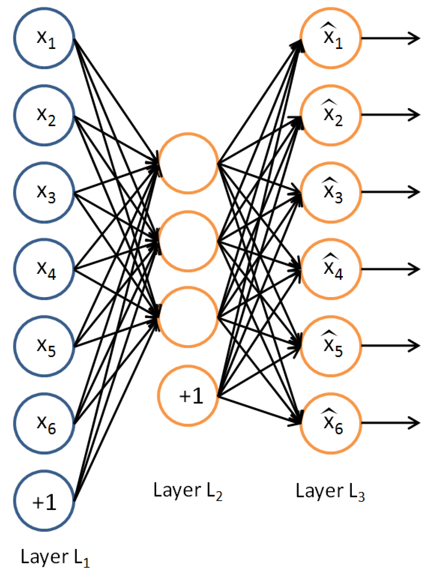
• We introduce three models based on stacked auto-encoders (AEs) to classify aspect categories in the Bangla language. In stacked learning, each layer of the network is trained separately to learn the encoding of the previous layer.
• As far as we know, stacked AEs have never been exploited in the task of aspect extraction in the Bangla language. In particular, in [7] the authors relies on standard machine learning algorithms, such as k-NN, SVM and random forest, while in [8] the authors propose a CNN with a single convolutional layer, max pooling, and a final standard classification layer, composed by a fully connected neural network and a softmax.
• We exploited AEs, contractive AEs, and sparse AEs, trained in the stacked fashion. All the proposed models show better precision, recall, and F1-score, with respect to the state-of-the-art works of Rahman et al. [7,8].
• Looking at the obtained results, it turns out that the stacked contractive AE, is the best model for aspect classification in the Bangla language.

Regarding the above points, we must specify the reasons behind the choice of AEs for aspect extraction. In the last years, researchers studied techniques that could both reduce the dimensionality in text classification and also improve the step of feature extraction, even called preprocessing. Vincent et al. [9], introduced denoising AEs: in their work, the authors add Gaussian noise to the original input and through the learning phase, the DAE can reconstruct the original input better than standard AEs. Bengio et al. [10] introduced the sparse AE. In such a model, only a few hidden units are allowed to be activated once. Sparsity is obtained considering additional terms in the reconstruction error function, in the training phase, or also by manually setting to zero k hidden units (indeed, we usually refer to k-sparse AE in the literature). Such work has hugely improved the feature extraction step and greatly improved classification performance.

As we said in the previous paragraphs, today, with the latest developments of the Web, a lot of data is available. The number of comments, opinions, and reviews of internet users has hugely increased and the most remarkable problem in SA is the classification of a huge amount of texts using feature spaces of high dimensionality [11,12,13]. In previous works related to ABSA in the Bangla language, researchers exploited many machine learning algorithms, such as k-NN, SVM, random forest and CNNs to classify sentences. Except for CNNs, researchers used handcrafted features widely used in the field of SA. For instance, they used Bag of Words representation [14], which can result in high dimensional representations, as the number of different involved words increase [15,16]. With CNNs, they built huge feature representations, sometimes difficult to handle from a training and a representative point of view. Since with ABSA we are dealing with huge dimensionality, reducing the feature space is a desirable choice. Further, an important point that has not been tackled in ABSA in the Bangla language is trying to use different feature representations, not common in the literature. We perform this step using AEs, which are powerful techniques for extracting features from spaces that present a high dimensionality.

The following work makes use of three AEs methods for the task of ABSA in the Bangla language to improve aspect classification performance with respect to [7,8]. As the authors did in such articles, we had to preprocess the sentences to remove some noise in the text (i.e., information not useful in performing the classification task), for instance, numbers, stop words and punctuation. Removing such elements reduces the feature space. Then, we represent the text using a Vector Space Model (VSM), proposed in Salton et al. [17]. The VSM is a model for representing documents (i.e., text documents and sentences) as a vector of identifiers. We will compute the identifiers according to several methods, that we are going to explain in the details in Section 3.

After choosing the representation, we have to carry the feature selection step. For such step, researchers used for instance mutual information [18], ${\chi }_2$ statistics [19] and many other metrics [20,21,22,23]. The problem with these criteria is that their parameters and thresholds are manually set. Most of the times it is difficult to set the right values and wrong settings may cause the deletion of useful features from feature space. A wrong feature selection can result in worse classification performance. To address the feature selection problem, we adopted AE models. Within the tested models, final experiments show that the stacked contractive AE gets the best performance in terms of precision, recall, and F1-score. The experiments show an average improvement of $0.17$, $0.31$ and $0.30$, across the restaurant and cricket datasets, respectively in precision, recall and F1-score.

The structure of the paper is as follows: in the next section, we present many related works that focus on ABSA both in Bangla and in other languages; in Section 3, we explain in the details which preprocessing we applied to the data, i.e., mainly which feature representation we used; in Section 4 we introduce the three models of AEs we employed; in Section 5 describe the experimental settings; in Section 6 we analyze and discuss the experimental results we obtained and finally, in the last section, we sum up the conclusions and we draw many future directions that can arise from the following work.

2. Related Works

In this section, we analyze the most remarkable works that address the problem of SA and ABSA both in Bangla and other languages. First, we consider many works in English language to see the current major trends, as English language is the language for which SA and ABSA are more tackled. Then, we also consider other languages for which relevant works and datasets are available. In the last paragraph, we finally take into account the most important works that focus on SA and ABSA in the Bangla language. More information can be found in wide survey papers such as [24,25].

Among the first works that are focused on ABSA in English language, there is the one from Ganu et al. [26]. The authors exploit the use of SVM for extracting the most relevant topics of sentences. In their work, they propose a manually labeled dataset of restaurant reviews that covers four domain-related topics and two miscellaneous topics. For each of such topics, the authors train a separate, and binary SVM classifier. As features, stemmed tokens are used. Results are evaluated through precision and recall values for each topic. For the four domain-related topics they achieve an averaged F-measure of $73.4$. Considering all the topics, the averaged F-measure decreases to $67.1$.

In the SemEval-2016 conference, the dataset by Ganu et al. is extended by adding three more aspects by Nakov et al. [5]: the authors added tweets, SMS messages and LiveJournal sentences with sentiment expressions annotated with contextual phrase-level and message-level polarity. On such dataset, given a message containing a marked instance of a word or a sentence, the task again consists of determining if that instance is negative, neutral or positive in such context. Even more languages are added in SemEval 2016 [6]. These languages are French, Arabic, Russian, Dutch, Turkish, Chinese and Spanish. Also, further aspects are added, such as “museum”, “mobile phone”, “laptop”, “hotel”, “digital camera”, and “telecommunication”.

For the Arabic language, we can find one of the most advanced datasets for ABSA. Such dataset is published in Al-Smadi et al. [27]: it consists of 2838 book reviews in Arabic language which have been annotated by humans with aspects and polarities. The authors, classified book reviews in 14 different aspects (For instance, time, author, feelings, context, rating, etc.) and they provided four different polarities (positive, negative, neutral, and conflict). Nevertheless, in the article baseline results are reported, and a common evaluation technique is proposed to facilitate the future evaluation of research and methods based on the dataset.

In Tamchyna et al. [28], a remarkable IT (Information Technology) product review dataset is proposed in Czech, for the task of ABSA. The dataset contained 2000 reviews in the form of short segments, with an average length of 30 characters, and long reviews, with an average length of 1000 characters. All the documents were manually tagged for both aspects and polarities by a single annotator. It one of the few datasets for which we have high variability in the length of the documents. This is an important aspect, as pointed out by the authors: the long reviews are more difficult to classify, for both aspects and polarities, than short segments. The best F1-score measure achieved on the short segments is $65.79$ while for long segments it is only $30.27$. The authors explain this point by underlying the lower density of aspect terms in long reviews, compared to the short segments.

On the mentioned datasets, many classification techniques were exploited in the context of ABSA. For instance, latent dirichlet allocation (LDA) [29] is one of the most used techniques in the classification of the aspects [24,25]. Many works use variations of LDA to discover latent topics in a collection of sentences or documents, with the hope that these topics will correspond to rateable aspects for the considered entity [30,31,32]. In Lu et al. [33], the authors investigated many unsupervised topic modeling approaches, LDA based, for the SA tasks of (1) multi-aspect sentence labeling, where each sentence in a document is labeled according to the aspects it is focused on, and (2) multi-aspect rating prediction, where the goal is to predict implicit aspect-specific star ratings for each sentence contained in a document. The authors obtained remarkable performance in both the tasks and suggest that, in combination, they can also support interesting applications for aspect-based review summarization. A probabilistic generative model named Sentence-LDA was introduced in Jo et al. [34]. The authors tackle the problem of automatically extracting which aspects are considered in reviews and how sentiments are conveyed for different aspects. The results show that the aspects discovered by sentence-LDA match evaluative details provided by the reviews and the method comes close to the performance of the state-of-the-art supervised classification methods. However, it is assumed that all the terms in a sentence are generated considering from a single aspect, which is a strong limitation. Recently, in Poria et al. [35], Sentic-LDA was proposed to improve the aspect and polarity classification performance in the task of ABSA: the authors, developed an LDA algorithm considering the semantic similarity between pairs of words, instead of only exploiting word frequency measures, thus, capable of extracting opinions and sentiments that are only implicitly expressed in a text and, overall, contributing to improved clustering.

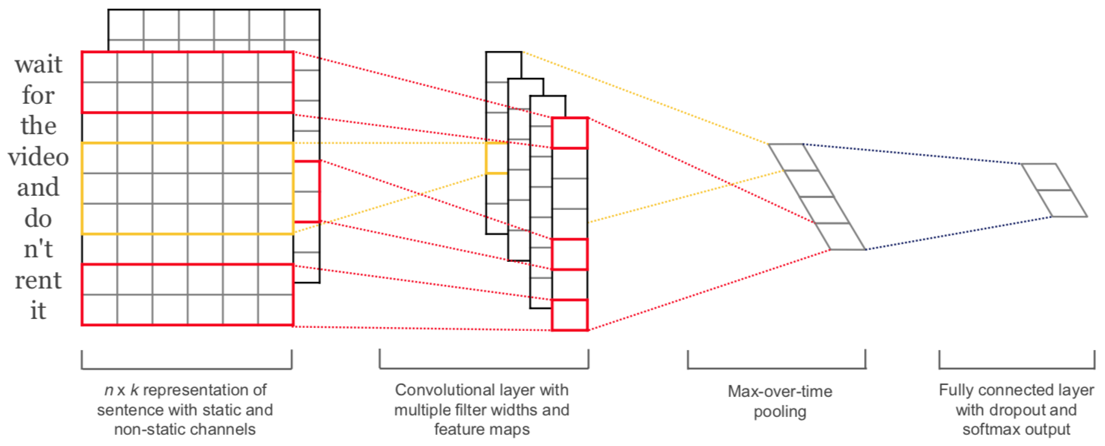
As in other research fields, deep learning and in particular CNNs were widely used in the field of ABSA [36]. For instance, a foundational article is one of Kim et al. [37]. The authors designed a CNN architecture and benchmarked it on several well-known ABSA datasets. The proposed CNN architecture achieves good performance despite it is surprisingly simple: the input layer is a sentence comprised of concatenated word2vec word embeddings [38]. This layer is followed by a convolutional layer with many filters, then a max-pooling layer, and finally a classification layer, composed by a fully connected neural network and a softmax. The architecture is reported in Figure 1 for clear visualization. Further, the authors exploit different channels with static and dynamic word embeddings, where only one channel is tuned during the training step and the other are fixed. A similar, but more complex architecture was previously proposed by Kalchbrenner et al. [39].

Differently from Kim et al., Johnson et al. [40] train a CNN from scratch, without exploiting pre-trained word vectors, like word2vec. The authors design an architecture in which convolutions are directly applied to one-hot encoding vectors. Further, a bag-of-words-like representation is proposed for the input data, both efficient in terms of space and capable of reducing the number of parameters of the network. In another work, the same authors extend the architecture with an additional unsupervised region embedding, learned using a CNN that predict the context of text regions [41]. If we analyze the results proposed by [40,41] we notice that the presented approaches obtain good performance for long texts (for instance, like book or movie reviews). However, their performance on short texts (like Facebook posts or tweets) is worse than the ones reported in Kim et al. [37]. It has been observed that using pre-trained word embeddings for short texts yields better performance than using the same for long texts [24,25].

Most of the architectures and approaches for ABSA rely on a unique classifier, which authors train on annotated data to recognize the aspect and the polarity of a document. We point out a few works that tackle ABSA through ensemble classifiers. In this view, Perikos et al. [42] propose a classifier ensemble approach: LDA is exploited for topic modeling and natural language processing techniques are used to catch the texts dependencies and determine interactions between texts and aspects. Then, an ensemble classifier schema based on Naive Bayes, maximum entropy and SVM base classifiers is designed to extract the polarities and then to classify the polarity of users’ opinions, with respect to the aspects they address. The evaluation results show that considering text dependencies help in the accurate classification of users’ opinions and also that the ensemble classifier schema performs robustly better than the individual base classifiers. Another work based on ensemble methods is one of [43]. The authors present a system is composed of two independent sub-systems: the sentiment polarity identification part and the aspect category detection part. The novelty of their approach consists of the architecture of the system: an ensemble of neural networks, and the usage of ConceptNet pre-trained word vectors (they are pre-trained word vectors like GloVe, word2vec or fastText). The method presented by the authors outperforms many state-of-the-art works that use a single base learner, or even complex neural network architectures.

Considering Bangla language, most of the works are focused only on SA. In Chowdhury et al. [44], the authors aim to automatically extract the sentiments conveyed by users from Bangla microblog posts and then identify their polarity as either negative or positive. An important point of the work is that it is used a semi-supervised bootstrapping approach for building the training dataset, which avoids the need for manual annotation. For classification, the authors use SVM and Maximum Entropy and provide a comparative analysis of the performance of such algorithms by experimenting with several combinations of various sets of well-known features. In Hasan et al. [45], the polarity of sentences (negative, neutral or positive) is classified using contextual variance analysis: In linguistics, the valence of a verb is the number of near nouns with which a verb combines. The proposed system first performs a parsing step to identify the parts of speech and then applies rules to assign contextual valence (the polarity) to the linguistic components. The main limitation of the work is that the scope of the paper is only limited to SA.

Regarding datasets for SA and ABSA in the Bangla language, few of them are publicly available online and the most are private. A remarkable dataset for SA is published in Hassan et al. [46]. The dataset is called “Bangla and Romanized Bangla Texts” (BRBT) dataset. The dataset consists of 9337 post samples and it is of high importance because it is the largest available one in Bangla, and also encompasses the till-now-ignored Romanized Bangla. Romanized Bangla is simply the Bangla language written using the English alphabet. However, the dataset is currently kept private (despite it may be made available by personally contacting the owner/authors, and signing a consent form). The authors employed an LSTM deep network obtaining high performance, but it is difficult to compare with their results because the dataset is private and the sharing is limited. The same dataset is used in Alam et al. [47] where a CNN is employed for classifying the polarity of the sentences (only negative or positive). The proposed model obtains a classification accuracy of $99.87\%$, which is $6.87\%$ better than the work of Hassan et al. [46]. Notice that all these works are focused only on the classification of polarity, as the employed datasets don’t come with information regarding the aspects.

As far as we know, the only two datasets in the Bangla language that come with aspect and polarity information are the ones published in Rahman et al. [7]. As we said in the Introduction section, the authors introduced two datasets named “cricket” and “restaurant”.

Regarding the cricket dataset, the authors collected manually 2900 comments from two online sources: BBC Bangla and the Daily Prothom Alo. They are very popular news websites in the Bangla language that publish trustworthy and authentic news. People from Bangladesh frequently read the posts and the news from these sources and often leave comments to share their opinion. Both the Facebook pages of BBC Bangla and Daily Prothom Alo have over 10 million followers and they provide a huge number of comments. Cricket has been chosen by the authors, as it is one of the most popular games in Bangladesh and they report that people are more interested in making comments on such sport, than on other topics. Here, we report some cricket-related sentences taken from Prothom Alo and BBC Bangla Facebook pages. We report the English translation of the sentences for better readability and understanding of everyone. For instance, this is a neutral polarity sentence for the aspect “team”, taken from Prothom Alo:

“Razzaq is recently playing well, but the mister is not giving a chance to him.”

Another sentence, taken BBC Bangla, for the aspect “batting” and with negative polarity is

“I don’t want to see Vijay in the national team anymore.”

The Bangla text on cricket is annotated jointly by the authors and many other people including a group of Bachelor students, and two employees from the Institute of Information Technology, University of Dhaka, Bangladesh. All participants agreed to categorize the whole dataset into five different aspects categories: betting, bowling, team, team management and other. Given a comment, the task of the annotators was to recommend the aspect category and polarity labels for each. Three types of polarities were considered, that is, positive, negative, and neutral. Each participant categorized every comment of the dataset. Finally, the authors applied a majority voting technique to make the final decision about the aspect category and the polarity of a sentence.

Regarding the Restaurant dataset, the authors took help directly from the English benchmark’s Restaurant dataset presented in SemEval-2014 by Pontiki et al. [6]: all the 2800 original sentences were translated into Bangla with their exact annotation. As in the original English dataset, five types of aspect categories are present, that are, food, price, service, ambiance, and miscellaneous. In terms of the polarity, the authors considered only three polarity labels, that is, positive, negative and neutral. The original dataset consisted of four different polarity labels: positive, negative, neutral, and conflict. In the translated Bangla dataset, the conflict category was omitted and it is assumed to be the same as the neutral category. Again, we show two examples of sentences that we can find in the dataset. The first one is representing the aspect “ambiance” with negative polarity:

“There are a very limited number of seats.”

The second one is representing the aspect “food” with negative polarity:

“The food was good, but not enough.”

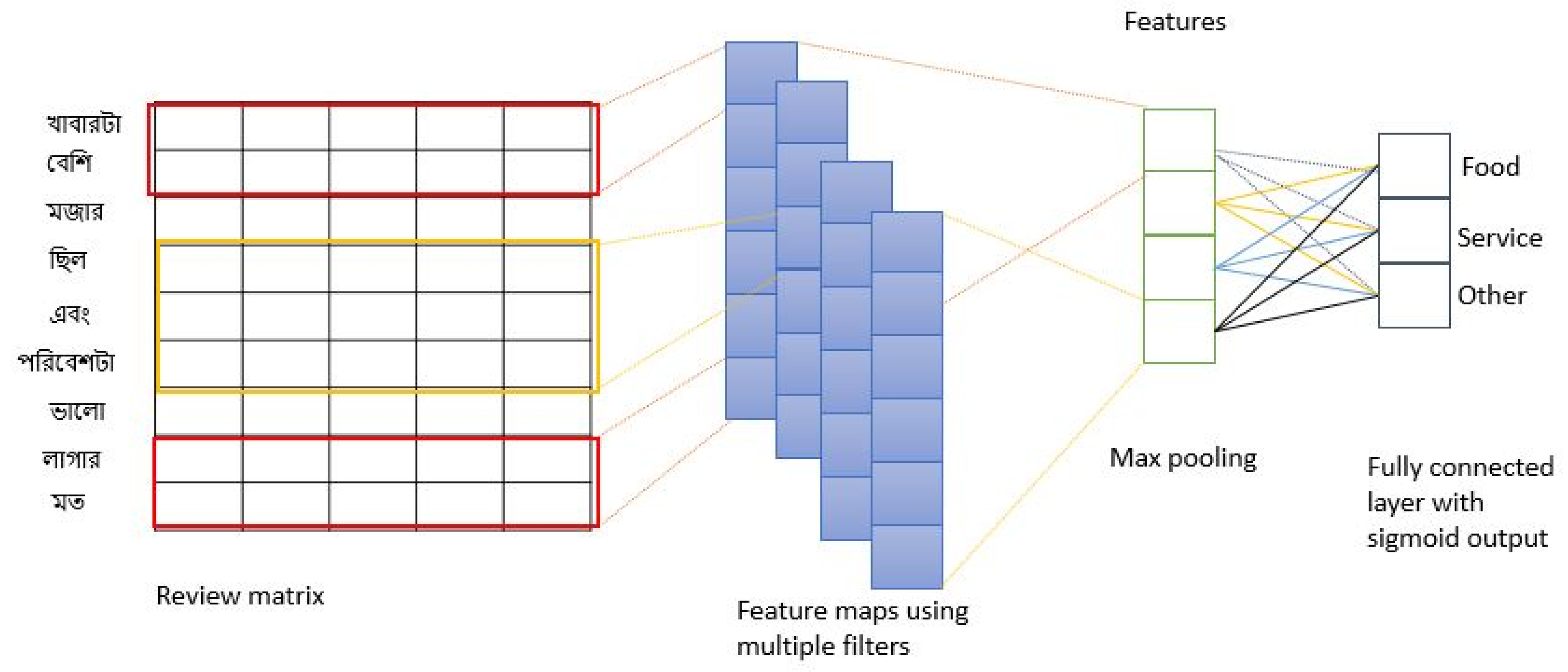
Baseline results exploiting k-NN, SVM, and random forests are provided by the authors for both the datasets [7]. The latter work is followed by the work [8] of the same authors. They classified aspects using a CNN and obtained better performance with respect to their previous article [7] in terms of recall and F1-score. The input layer is a sentence comprised of concatenated word2vec word embeddings [38] and the network consists of a unique convolutional layer followed by a max-pooling and finally a classification layer, composed by a fully connected neural network and a sigmoid. The architecture of the proposed CNN shown in Figure 2.

3. Preprocessing

In this section, we describe which preprocessing and which features we extracted from the sentences contained in the two datasets provided by Rahman et al. [7]. We specify that we performed the same preprocessing steps and we extracted the same features from the sentences for both the cricket and the restaurant datasets. As the authors did in such articles, we had to preprocess the sentences to remove noise in the text (i.e., information not useful in performing the classification task), for instance, numbers, stop words and punctuation. We remark that this step was performed in the majority of the works we analyzed and it has been experimentally tested that it doesn’t reduce classification performance: it has been experimentally tested that elements such as numbers, stop words and punctuation are not useful in the classification of the aspects, as intuitively one can imagine [24,25]. Further, the removal of such elements implies a reduction of the dimensionality of the feature space.

After the preprocessing step where noise is removed, we represent the text using a vector space model (VSM), proposed in Salton et al. [17]. The VSM is a model for representing text documents and sentences as a vector of identifiers. It is one of the most used models for representing texts and it is simple to implement and to understand. A document d (i.e., a sentence or a longer text) is represented as the vector

$$d=(w_1,w_2,\cdots ,w_t),$$

where $w_t$ corresponds to the weight w that is given to the t-th term contained in the document d. Many ways have been studied to compute the weights. One of the most used is the Term frequency-inverse document frequency (TFIDF) [48] representation: it was introduced by Salton et al. [49] and it leads good performance when used as feature representation in the fields of ABSA, but also in many tasks across the fields of Information Retrieval and Text Mining. The TFIDF representation is based on two concepts:

• If the frequency of a term in a specific document is higher than other terms, such term better distinguish the document, with respect to the other categories (the aspects in ABSA).
• If a term appears with high frequency in all the documents, it means that is not able to distinguish between the categories which the documents belong to (this is the case of articles, for instance, the articles “the”, “a”, and “an”, that are common in almost all the sentences).

According to the first point, the weight of a term is proportional to the term frequency (TF), while according to the second point the specificity of a term can be computed as the inverse function of the number of documents in which the term is contained, i.e., the inverse document frequency (IDF). Hence, TFIDF is the product of the two mentioned statistics and is defined as:

$$TFIDF(t,d,D)=TF(t,d)\times IDF(t,D),$$

where t is a term contained in a document d and D is the set of all the documents. Considering a document $d\in D$, for every term t contained in it we compute $w_t$ as

$$w_t=TFIDF(t,d,D).$$

The most simple and the most common definitions of TF and IDF are:

$$\begin{array}{cc}\hfill TF(t,d)& =f_{t,d},\hfill \end{array}$$

(1)

$$\begin{array}{cc}\hfill IDF(t,D)& =log\frac{N}{n_t},\hfill \end{array}$$

(2)

where $f_{t,d}$ is the row count of the term t in the document d, i.e., the number of times that the term t occurs in the document d, $N=\left|D\right|$ and $n_t=\left|\{d\in D:t\in d\}\right|$, i.e., the number of documents in which the term t appears. To understand better the concept of TFIDF, consider a document d containing 100 words, in which the term t is contained 5 times. Hence, $TF(t,d)=\frac{5}{100}=0,05$. Now, let’s assume we have 1000 documents in our set D and the term t appears in 10 of them. It turns out that $IDF(t,D)=log\frac{1000}{10}=2$. We can compute the TFIDF value for the term t in the document d contained in the set D as $TFIDF(t,d,D)=0.05\times 2=0.1$.

We exploited several TFIDF definitions, according to the ones that are most used in the literature [50]. We considered the classical one where TF and IDF are defined respectively as (1) and (2), and further the following ones:

$$\begin{array}{cc}\hfill TFID{F}^{\prime }(t,d,D)& =(1+log\left(f_{t,d}\right))\times log\frac{N}{n_t},\hfill \\ \hfill TFID{F}^{″}(t,d,D)& =\left(0.5+0.5\frac{f_{t,d}}{{max}_{\{t^{\prime }\in d\}}{f}_{t^{\prime },d}}\right)\times log\frac{N}{n_t},\hfill \end{array}$$

where the first therm of the above products stands for TF and the second term for IDF respectively.

We computed features according to a VSM model, where weights are computed exploiting three different TFIDF definitions. We could consider many other feature representations, for instance one of the most used as an alternative to TFIDF is bag of words (BoW) [14]: it first computes a vocabulary extracting unique words from the documents and returns a vector representation with term frequencies (absolute or relative frequency) for each term contained in the corresponding document. BoW carries several drawbacks. In particular, we avoided its use for the following reasons:

• The ordering of the terms was not considered in BoW representation.
• The specificity of a term is not considered. Only the absolute or relative frequency was considered.
• The dictionaries resulting from the two considered datasets were huge.
• The dimension of the computed dictionaries could result in a network of too high dimensionality for the sizes of the given datasets, that are around a few thousands of sentences.

4. Auto-Encoder Based Models

We employed three different models of AEs in the present work. We made use of standard AEs, contractive AEs (CAEs) and sparse AEs (SAEs). As far as we know, AEs have never been exploited in the task of aspect extraction in the Bangla language. In particular, as we have seen, in [7] the authors rely on standard machine learning algorithms, such as k-NN, SVM, and random forest, while in [8] the authors propose a CNN architecture, presented in Figure 2.

In this section, we describe in the details the three AEs based architectures we propose, in particular, the standard AE, as the other architectures are strictly related to it.

4.1. Standard Auto Encoders

AEs are neural networks introduced by Rumelhart et al. [51,52]. While conceptually simple, they play an important role in machine learning. AEs were first introduced in the 80 s by Hinton and the PDP group. The authors showed how to use backpropagation to learn features with lower dimensionality than the input ones in an unsupervised manner, and then how to use them to reconstruct the original high dimensional input. Hence, AEs learn a sort of identity function, where the output must be as similar as possible as the input, according to an error measure. We can think AEs as simple learning circuits whose goal is to transform inputs into outputs with the least possible amount of distortion, i.e., the reconstruction error.

Recently, AEs are highly considered among the deep learning approaches where AEs, in particular restricted Boltzmann machines (RBMS), are first stacked and then trained bottom-up in an unsupervised fashion, followed by a supervised learning phase to train the top layer and fine-tune the entire architecture. This bottom-up phase is completely agnostic with respect to the final task (for instance a multi-class classification). Thus, it can be used in transfer learning approaches. Several times, these deep architectures lead the state-of-the-art results on a wide number of challenging classification and regression problems [53,54,55,56,57].

An example of standard AE is shown in Figure 3. It is composed by an input layer ($L_1$), a hidden layer ($L_2$), and an output layer ($L_3$).

Considering the example of Figure 3, the input is represented by the vector $\mathit{x}=[x_1,x_2,\cdots ,x_6]$. The elements of the vector can represent the input data or even the features extracted from the data. The output is represented by the estimate $\widehat{\mathit{x}}=[{\widehat{x}}_1,{\widehat{x}}_2,\cdots ,{\widehat{x}}_6]$. The AE network learns an approximation function $\mathit{x}\approx \widehat{\mathit{x}}$, i.e., the AE learns a function that is capable of reconstructing the output as much as similar to the input, according to a dissimilarity or a distortion function (e.g., $L_p$ norm, Hamming distance) defined over the input and output space, which is commonly named as reconstruction error. The AE is composed by an encoding step and a decoding step:

• Encoding step: it is performed by the input layer and the hidden layer. In the encoding step we considered a training set $\mathit{X}=\{{\mathit{x}}_1,{\mathit{x}}_2,\cdots ,{\mathit{x}}_m\}$, where assume that ${\mathit{x}}_i\in R^{D_x}$, for $1\le i\le m$, and $D_x$ is the dimension of the samples contained in the training set $\mathit{X}$. The hidden layer activation function is usually set as the sigmoid function, defined as

  $$\sigma \left(z\right)=\frac{1}{1+e^{-z}},$$

  but many other functions can be used. The output $\mathit{h}$ of the neurons in the hidden layer is computed as

  $$\mathit{h}=f\left(\mathit{x}\right)=\sigma (\mathit{W}\mathit{x}+\mathit{b}),$$

  where $h\in R^{D_h}$, $\mathit{W}\in R^{D_h\times D_x}$ is the weight matrix between the input and the hidden layers (it contains the weights associated to each arch), and $\mathit{b}\in R^{D_h}$ is the bias vector. Hence, the input data has been encoded as $\mathit{h}$. The following step is the decoding one, i.e., decode such representation and reconstruct the original input, minimizing the reconstruction error.
• Decoding: the decoding process is performed by the hidden layer and the output layer. The reconstructed output $\mathit{r}\in R^{D_x}$ is computed as

  $$\mathit{r}=g\left(\mathit{x}\right)=\sigma ({\mathit{W}}^{\prime }\mathit{h}+{\mathit{b}}^{\prime }),$$

  where $\mathit{r}$ is reconstructed for approximate the input $\mathit{x}$, ${\mathit{W}}^{\prime }\in R^{D_x\times D_h}$ is the weight matrix and ${\mathit{b}}^{\prime }\in R^{D_x}$ is the bias vector.

During the training step, the AE updates the weight matrices $\mathit{W},{\mathit{W}}^{\prime }$ and the bias vectors $\mathit{b},{\mathit{b}}^{\prime }$ to get the minimum reconstruction error. Considering any definition of reconstruction error we take into account, it is clear that the minimum reconstruction error is reached when the output is identical to the input. Usually, the reconstruction error function is defined as:

$$J_{AE}(\Theta )=\sum _{\mathit{x}\in {\mathit{X}}^{\prime }}L(\mathit{x},g\left(f\left(\mathit{x}\right)\right)),$$

(3)

where $\Theta =\{\mathit{W},\mathit{b},{\mathit{W}}^{\prime },{\mathit{b}}^{\prime }\}$ is the set of parameters, ${\mathit{X}}^{\prime }=\{{\mathit{x}}_1^{\prime },{\mathit{x}}_2^{\prime },\cdots ,{\mathit{x}}_{m^{\prime }}^{\prime }\}$ is the test set, and L is the reconstruction error function. Such function is usually expressed as an $L_p$ norm. For instance, if we set $p=2$, the reconstruction error function L is defined as

$$L(\mathit{x},\mathit{r})=\left|\right|\mathit{x}-{\mathit{r}\left|\right|}^2=\left|\right|\mathit{x}-{g\left(f\left(\mathit{x}\right)\right)\left|\right|}^2,$$

which is the usual Euclidean norm.

4.2. Contractive Auto Encoders

In the last years, many AEs were introduced, where advancements have been proposed both in the architecture and in the use of different reconstruction error functions. One of these is the CAE, introduced by Bengio et al. [58]. The authors proposed a new reconstruction error function where a penalty term is added to the traditional reconstruction error (3): they summed to it the Frobenius norm of the Jacobian matrix of the input sample $\mathit{x}$. The Frobenius norm of the Jacobian matrix of the hidden layer is computed with respect to the input sample $\mathit{x}$ and is the sum of the square of all elements. It is computed as

$$\begin{array}{c}\hfill \left|\right|J_f\left(\mathit{x}\right){\left|\right|}_F^2=\sum _{ij}{\left(\frac{\partial {\mathit{h}}_j\left(\mathit{x}\right)}{\partial {\mathit{x}}_i}\right)}^2.\end{array}$$

(4)

With this trick, the CAE makes the encoding less sensitive to small variations in the training set. This is simply to exploit and implement, as it is simply achieved by adding the regularizer, or penalty term, of (4) to the reconstruction error function the network is minimizing. The final result is that the CAE can reduce the learned representation’s sensitivity, towards the training input. Further, such penalty force the mapping of the feature space to not increase in dimension. Keeping the feature space of low dimension allow CAEs to be more robust when the input data are corrupted by noise. This also allow to build more robust feature representations. The CAE reconstruction error function is defined as follow:

$$\begin{array}{cc}\hfill J_{CAE}(\Theta )& =\sum _{\mathit{x}\in {\mathit{X}}^{\prime }}(L(\mathit{x},g\left(f\left(\mathit{x}\right)\right))+\lambda ||J_f{\left(\mathit{x}\right)\left|\right|}_F^2),\hfill \end{array}$$

where $\Theta$ and ${\mathit{X}}^{\prime }$ are respectively the set of parameters and the test set, defined as above. The CAE surpasses the results obtained by other AE architectures regularized with weight decay or by denoising [9]. The CAE sometimes is a better option than denoising autoencoder to learn useful feature extraction [58].

4.3. Sparse Auto-Encoders

Neural networks, also any kind of AE, are initialized with random weights usually sampled from a standard Normal distribution. Computing back-propagation on a randomly initialized network can result in slow learning and it is easy to get stuck in local minima with low performance. Many works tackled such problem, in particular, G. Hinton showed that an unsupervised pre-training of the layers for learning a sparse representation, before the classification task, reduces the mentioned issue [50].

A SAE considers an input vector and learns a dictionary that transforms the input to another representation. In such model, a layer of the network learns a dictionary that minimizes the reconstruction error and tries to employ the less number of elements in the code for reconstruction.

The most simple SAE is composed by a unique hidden layer, $\mathit{h}$, where the input $\mathit{x}$ is transformed in a sparse representation and then reconstructed as $\widehat{\mathit{x}}$. The learning phase is carried as the standard AEs, through the minimization of the reconstruction error. Sparse autoencoders have usually a number of hidden nodes greater than input nodes. In the literature, we refer to these models as k-SAEs, where are considered only the k highest activations in $\mathit{h}$ and the others are set to zero. This prevents the model to make use of all of the hidden units at a time and forcing only a reduced number of hidden nodes to be used. The error is then only back-propagated through the k considered nodes in $\mathit{h}$. This constraint is represented as a sparsity penalty function, $\Omega \left(\mathit{h}\right)$, which is applied on the hidden layer $\mathit{h}$ and summed to the reconstruction error. Hence, the reconstruction error function is the following:

$$\begin{array}{cc}\hfill J_{k-SAE}(\Theta )& =\sum _{\mathit{x}\in {\mathit{X}}^{\prime }}\left(L(\mathit{x},g\left(f\left(\mathit{x}\right)\right))\right)+\Omega \left(\mathit{h}\right),\hfill \end{array}$$

where, again, $\Theta$ and ${\mathit{X}}^{\prime }$ are respectively the set of parameters and the test set, defined as above. A complete explanation of the model can be found in [59].

5. Experimental Settings

In this section, we describe the experimental settings we set for evaluating the proposed models. In the next section, we focus on analyzing the results we obtained and we will critical discuss them with respect to the state of the art works that tackled the problem on the same dataset [7,8].

For the feature selection step, we used a VSM model, where each sentence d contained in the two datasets (cricket and restaurant) is encoded as

$$d=(w_1,w_2,\cdots ,w_t),$$

where $w_t$ corresponds to the weight that is given to the t-th term contained in the sentence d. We exploited three different TF-IDF criteria we presented in the previous sections:

$$\begin{array}{cc}\hfill TFIDF(t,d,D)& =f_{t,d}\times log\frac{N}{n_t},\hfill \end{array}$$

(5)

$$\begin{array}{cc}\hfill TFID{F}^{\prime }(t,d,D)& =(1+log\left(f_{t,d}\right))\times log\frac{N}{n_t},\hfill \end{array}$$

(6)

$$\begin{array}{cc}\hfill TFID{F}^{″}(t,d,D)& =\left(0.5+0.5\frac{f_{t,d}}{{max}_{\{t^{\prime }\in d\}}{f}_{t^{\prime },d}}\right)\times log\frac{N}{n_t},\hfill \end{array}$$

(7)

where the first part of the above products is TF and the second part is IDF respectively. The length of the VSM representation for each sentence is variable, as usually different sentences contain a different number of terms. Hence, we zero-padded every VSM representation to the length of the two maximum length sentences contained in the two datasets. Respectively, the VSM representations of the sentences contained in the restaurant dataset are zero-padded to a length of 51 and the VSM representations of the sentences contained in the cricket dataset are zero-padded to a length of 34.

As after the zero-padding the length of the VSM representations of the sentences contained in the two datasets turns out to be different, we built two different AEs architectures with 51 and 34 neurons in the input layers, respectively for the Restaurant and cricket dataset. We used two hidden layers where the dimension is respectively set to 20 and 10 neurons after several experiments, for both the architectures. In the end, a Softmax layer is set in both the networks for classifying among five classes (food, price, service, ambiance and miscellaneous for the restaurant dataset; betting, bowling, team, team management and other for the cricket dataset). We remark that, apart from the size of the input and output layer, the proposed architecture for the Restaurant and the cricket dataset are the same. This was required because of the different lengths of the VSM representations for the two datasets.

We exploited three different AE models for the two used datasets, i.e., standard AEs, CAEs, and k-SAEs. We remark that the architecture of the six tested models, i.e., the number of levels and neurons, is the same, but the error function changes with respect to the adopted model. For all the models, we employed sigmoid activation functions for all the neurons, Adam as adaptive learning rate optimization and we trained for 1000 epochs. We set the k-SAE k values in the range from 1 to 10, with a step of 1. We trained the networks in a stacked fashion, i.e., we trained each layer separately to learn the encoding of the previous layer and according to a 10 fold stratified cross-validation. This is one of the effective ways to train a neural network, introduced in Vincent et al. [9]. The authors showed that training stacked layers allow learning suitable representations in a better incremental way, instead of training the entire network, where all the weights are initialized randomly. For instance, consider the networks we built for the restaurant dataset. We remark that we train in the same way the networks we proposed for the cricket dataset. In the details we:

• Trained the first hidden layer: we trained an AE with one hidden layer of size 20 and with input and output layers of size 51.
• Trained the second hidden layer: we trained an AE with one hidden layer of size 10 and with input and output layers of size 20. With this second learning phase, we are learning the weights of the second hidden layer for reproducing the representation previously learned with the first hidden layer.
• Trained the Softmax classifier: we trained a neural network classifier with an input layer that is the second hidden layer of the entire architecture and a Softmax classifier.
• Fine-tuning: we put together all the elements we trained separately and we performed a fine-tuning, i.e., we performed an entire learning phase starting from the weights we learned in the previous separate learning phases. This turns out to be better than train the whole architecture from completely random weights [9].

The models were created and trained using TensorFlow 1.14 under Python 3.7. The preprocessing was carried out using Pandas library, version 0.25 and standard Python 3.7 libraries. Since we didn’t have the necessary computational power to train the 6 different architectures in a 10 fold cross-validation setting, we relied on Amazon Web Services: we made use of an Amazon EC2 P3 instance. In particular, we used a p3.8xlarge instance with 4 Nvidia Tesla V100 GPUs, 64 GB of Ram memory, and 32 Intel Xeon Skylake vCPUs.

6. Experimental Results

In this section, we analyze the results we obtained and we critically compare them with respect to the state-of-the art works of Rahman et al. [7,8]. We compare our results in terms of precision, recall and F1-score as the considered datasets are highly unbalanced. We could also consider accuracy as an evaluation metric, but it can be misleading in cases such as the one we are analyzing, where the datasets are unbalanced. Also Rahman et al. compute accuracy measures in their works, but they do not take into account them for the same reasons we explained. We briefly mention that precision, recall, and F1-score are computed as follows:

$$\begin{array}{cccccc}\hfill \mathrm{Precision}& =\frac{\mathrm{TP}}{\mathrm{TP}+\mathrm{FP}}\hfill & \hfill \mathrm{Recall}& =\frac{\mathrm{TP}}{\mathrm{TP}+\mathrm{FN}}\hfill & \hfill \mathrm{F}1-\mathrm{Score}& =\frac{2\ast \mathrm{Precision}\ast \mathrm{Recall}}{\mathrm{Precision}+\mathrm{Recall}}.\hfill \end{array}$$

We report in

Table 1. Comparison between the performance reported in Rahman et al. [7,8] with the ones we obtained. We obtain better performance in terms of precision, recall and F1-score. The contractive auto-encoder (CAE) model is the model that achieved the best performance under every considered metric.

Dataset	Model	Precision	Recall	F1-Score
Cricket	CNN [8]	0.54	0.48	0.51
	SVM [7]	0.71	0.22	0.34
	RF [7]	0.60	0.27	0.37
	KNN [7]	0.45	0.21	0.35
	AE	0.79	0.70	0.74
	CAE	0.93	0.85	0.88
	SAE	0.88	0.82	0.84
Restaurant	CNN [8]	0.67	0.61	0.64
	SVM [7]	0.77	0.30	0.38
	RF [7]	0.69	0.31	0.38
	KNN [7]	0.54	0.34	0.42
	AE	0.82	0.74	0.77
	CAE	0.90	0.85	0.87
	SAE	0.85	0.82	0.83

the precision, recall and F1-score measures obtained by us and by the works [7,8]. The metrics were computed after a 10 fold stratified cross-validation. A 10 fold stratified cross-validation was a fair estimate that ensures the robustness of the introduced models, as we exploit many training and test sets and we do not rely only on a unique training/test split. Further, we make use of the stratification process that consists of rearranging the data to ensure that each fold is a good representative sample of the whole dataset. This approach ensures that one class of data is not overrepresented especially when the target variable is unbalanced. The value of 10, selected for the number of the folds, is a quite common value in the literature of machine learning: several relevant works found, from an experimental point of view, that 10 folds provide fair estimates with respect to bias and variance. An important paper that addresses this topic is Kohavi et al. [60]. Regard this point, we report that both in the articles of Rahman et al. it is not written which percentage and which data were used for training and test sets. With a 10 fold stratified cross-validation we ensure the reliability of our results.

Analyzing the work [7], we can see that SVM obtained the highest precision rate of $0.71$ and $0.77$ respectively for the cricket and the restaurant datasets. We further see that every baseline method the authors propose achieve low recall and then low F1-score. Analyzing the work [8], we notice that the CNN the authors proposed obtain different performance with respect to the baseline classifiers. Despite the precision being higher for SVM, the proposed CNN shows the highest recall and F1-score rates with a huge margin for both datasets. From the result, we can say that the CNN model identifies better aspect categories than the baseline machine learning approaches. It is clear from Table 1 that for most of the cases precision and recall shows different results. For this reason, we may check the F1-score, computed as the harmonic mean of precision and recall. The proposed CNN achieved the highest F1-score in both the datasets: on the cricket dataset it showed $0.51$ F1-score, whereas on the Restaurant dataset it showed $0.64$ F1-score.

Analyzing our work, we notice that all the three AE models we propose show better precision, recall, and F1-score than with respect to the methods proposed in the works of Rahman et al. [7,8], where standard machine learning approaches and a CNN were used. Despite we considered three different $TFIDF$ functions for computing weights for the VSM model, we report the performance only according to the $TFID{F}^{‴}$, reported in Equation (7), since it resulted as the best TF-IDF feature extraction method, which leads to the best performance. This turned out to be a flexible and compact representation, with respect to BoW used in [8]. Results for k-SAE are reported with k set to 7, as it was found to be the best value among the values from 1 to 10, with a step of 1. Despite precision is high for the SVM model, the proposed AEs provide better performance on both the datasets. The same holds for recall and F1-score: with the proposed architectures we outperform the CNN proposed by Rahman et al.. From the obtained results, we notice that the proposed models can classify aspect categories better than the previous approaches of [7,8], under every performance metric.

The experimental results show that CAE is the best model in accordance with the selected metrics. It is a robust approach for feature extraction and it improves classification performance. We report a $0.91$ and a $0.87$ F1-score on cricket and restaurant datasets respectively. Finally, we must notice in

Table 2. Comparison between the three proposed models when we train them in the standard way and with the stacked fashion. We notice that the architectures trained in the stacked way get the best performance.

Dataset	Model	Precision	Recall	F1-Score
Cricket	AE	0.71	0.64	0.67
	CAE	0.89	0.77	0.82
	SAE	0.80	0.75	0.77
	AE—stacked trained	0.79	0.70	0.74
	CAE—stacked trained	0.93	0.85	0.88
	SAE—stacked trained	0.88	0.82	0.84
Restaurant	AE	0.73	0.67	0.69
	CAE	0.84	0.81	0.82
	SAE	0.79	0.72	0.75
	AE—stacked trained	0.82	0.74	0.77
	CAE—stacked trained	0.90	0.85	0.87
	SAE—stacked trained	0.85	0.82	0.83

the improvement in performance when we train the models with the stacked fashion: from Table 2, it is clear that we have an improvement in performance when we train the methods with the stacked fashion. As remarked in the previous sections, the stacked training is a valid training framework that many times it achieves better performance than the standard one. It learns more suitable representations by training the architectures level by level, avoiding to train the network from completely random weights.

7. Conclusions

ASBA in the Bangla language is becoming an important problem, as online shopping and the use of the Web is more and more popular today in Bangladesh. Due to the rapid spreading of technology, people are using the Web in every aspect of their lives. Analyzing reviews, comments and opinions in the Bangla language is becoming fundamental, as people would like to purchase products online after considering the ideas of other customers.

As far as we know, only two datasets are released in the Bangla language for the task of ABSA. The first dataset is composed of restaurant reviews, while the second one is composed of comments and posts related to the sport of cricket. Such datasets are made available to benchmark both the tasks of aspect and polarity classification in ABSA. Basing on these datasets, we introduced three models based on AEs to tackle the task of aspect classification. We trained these architectures in a stacked fashion and we compared them with the previous approaches proposed in the literature. The experiments show that the proposed architectures obtain better performance with respect to the previous models. In particular, the CAE model obtains the best performance with $0.91$ and a $0.87$ F1-score on cricket and restaurant datasets respectively and it turns out to be the best model for aspect classification in Bangla.

In the next works, we plan to perform both aspect and polarity classification and to compare also with many other works and other datasets in the Bangla language, as polarity classification has been faced many times in the Bangla language. This is fundamental to tackle the complete task required from ABSA. Further, we want to experiment with several machine learning models and architectures. For instance, given the special characteristics of the task of ABSA, ensemble classifiers can be a quite suitable approach to be exploited to increase the performance of individual base classifiers we have used. Ensemble classifiers combine many base learners and can yield better generalization performance on unseen data, and report better performance compared to base learners.

We also want to investigate the explainability point of view. Most of the CNNs architectures, like the one proposed by Rahman et al., learn embeddings (low-dimensional representations) for words and sentences during the training phase. The majority of such articles don’t focus on investigating how meaningful the learned embeddings are. In [61] it is presented a CNN architecture that predicts hashtags for Facebook posts and at the same time, it is able to generate meaningful embeddings for words and sentences. These learned embeddings are proven to be meaningful and have been then successfully applied to other tasks. We want to rely on this article in the following works, to provide architectures that are also explainable and which aim is not only to provide good performance.

Finally, the last point we want to address is the data collection, from a qualitative and quantitative point of view. One of the datasets named cricket is collected from user comments on Facebook pages. In cricket related posts, the users share comments also not related to the cricket domain, i.e., they comment about politics or about the private life of cricket players. These kinds of comments are not categorized properly within the selected five aspect categories. Hence, these comments are included in the dataset as “other”, which may reduce the quality of the dataset. We want to develop more the dataset proposing more aspect classes, and further enlarge it taking the help of the automatic tools for web crawling. This can allow us to collect in a simply way thousand of sentences to improve the available datasets in the Bangla language.