A High Resolution Dataset of Drought Indices for Spain

Abstract

Drought indices are essential metrics for quantifying drought severity and identifying possible changes in the frequency and duration of drought hazards. In this study, we developed a new high spatial resolution dataset of drought indices covering all of Spain. The dataset includes seven drought indices, spans the period 1961–2014, and has a spatial resolution of 1.1 km and a weekly temporal resolution. A web portal has been created to enable download and visualization of the data. The data can be downloaded as single gridded points for each drought index, but the entire drought index dataset can also be downloaded in netCDF4 format. The dataset will be updated for complete years as the raw meteorological data become available.

Data Set: http://monitordesequia.csic.es/

Data Set License: ODbL 1.0

1. Introduction

Land degradation can be triggered by both natural and human factors, with the latter usually attributed to several processes including overexploitation and poor land management [1]. However, climate variability can also be an important factor triggering land degradation, either directly or coupled with other perturbation factors including overgrazing. Among the climate factors, drought is usually considered to be one of the most important [2,3].

Drought is one of the main natural hazards impacting on economic sectors and natural systems [4]. Although droughts have important socioeconomic and environmental components, they usually have a climate origin. For this reason drought analysis and monitoring is usually based on meteorological information as the main (or only) input, as it is widely available worldwide. Increasing drought severity associated with reduced precipitation and/or greater atmospheric evaporative demand (AED) is thought to be one of the most important drivers of land degradation in vulnerable regions (e.g., [5,6]).

Quantifying the effects of droughts is less direct than for other natural hazards, primarily because of difficulties in establishing the beginning, end, and duration of droughts, and the area affected [7]. For this reason, various indices have been developed to measure drought. These indices are essential for quantifying drought severity and assessing drought impacts, but also for developing drought monitoring systems that enable better preparedness and mitigation of drought risks [8].

The various drought indices differ in their characteristics and calculation procedures [9,10,11]. They vary from the simplest, which are based only on precipitation data [12], to the most elaborate, refined, and accurate, such as those that take into account AED [13].

Spain is highly affected by droughts [14,15], and various major drought episodes occurred during the 20th century, some of which affected the country for several years [16,17]. Droughts in Spain have severe economic impacts [18], including affecting the availability of water resources [19], causing forest decline and mortality [20,21], reducing vegetation activity [22], and causing failures in crop yields [23]. For these reasons the availability of accurate drought information is essential to better quantify drought impacts and to enable the assessment of drought risks in various economic sectors and natural systems.

The objective of this study was to describe a newly developed high spatial resolution drought dataset for Spain, based on various drought indices and covering the period 1961–2014.

2. Dataset Description

Seven drought indices are included in the dataset. Four of these are based on different versions of the self-calibrated Palmer drought indices: the self-calibrated Palmer Drought Severity Index (scPDSI), the Palmer Hydrological Drought Index (PHDI), the modified Palmer Drought Severity Index (WPLM), and the Palmer Z index. The other three drought indices are the Standardized Precipitation Index (SPI), the Standardized Precipitation Evapotranspiration Index (SPEI), and the Standardized Palmer Drought Index (sPDSI). The latter three indices are provided at 1-, 3-, 6-, 9-, 12-, 24-, 36- and 48-month time scales for visualization, but all time scales from 1 to 48 months are available for download. The data was generated at a spatial resolution of 1.1 km and at four time steps each month (Days 1–8, 9–15, 16–22, and from Day 23 to the end of the month), and is separated in two datasets. The first dataset covers Peninsular Spain and the Balearic Islands (PSBI) (35.75°N, 10.24°W to 43.99°N, 4.13°E), and the second covers the Canary Islands (CI) (27.86°N, 16.42°W to 29.00°N, 13.19°W). Both datasets are projected in the zone 30 North Universal Transversal Mercator coordinate system using the ellipsoid ED50. There are independent files for each dataset, and for each drought index and time scale. The files are available in Network Common Data Form 4 (NetCDF4) format. Currently, the data are available from 1961 to 2014, but the datasets will be updated by complete years as the raw meteorological data become available.

3. Material and Methods

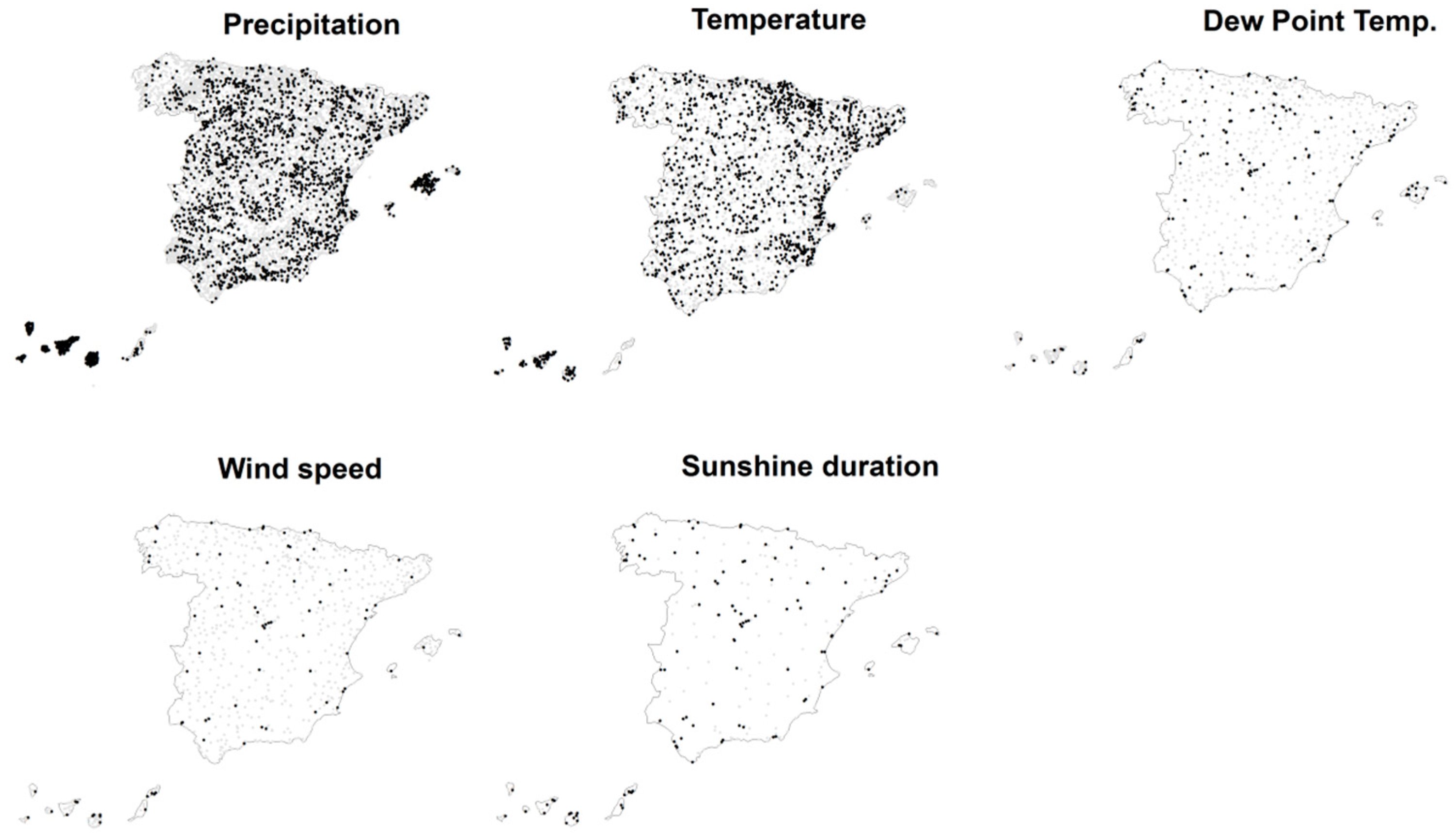
3.1. Data Acquisition and Processing

Daily meteorological data on precipitation, maximum and minimum temperature, relative humidity, wind speed, and sunshine duration (as a surrogate variable for incoming solar radiation) were obtained from the National Spanish Meteorological Services (AEMET) archives for the 1961–2014 period. Precipitation is the key meteorological variable that determines drought severity, but the other variables are needed to quantify AED, which is used in most of the drought indices. The initial dataset included information from 10,718 stations for precipitation, 5110 for temperature, 1131 for relative humidity, 353 for sunshine duration, and 979 for wind speed. The extent of temporal coverage varied amongst the variables: there were limited data available on relative humidity, sunshine duration, and wind speed prior to the 1990s.

Daily data were subject to careful quality control, which included identification of spurious data, repeated records, and coding errors (see details in [24]). Daily series were converted to weekly series. The sum of daily values was used for precipitation, while for the other variables the weekly mean was estimated with an allowance for only one day of missing data. Relative humidity and temperature data were combined to calculate the dew point temperature, which was used in the following steps of the process. As drought indices are relative metrics and their calculation requires homogeneous time periods, it was not possible to use “week” as the reference time step for calculations because the first day of each year can fall on different days, and this propagates through the entire year. The occurrence of leap years also potentially increased the inhomogeneity of the periods to be compared. For this reason, each month was divided into four artificial “weekly” periods, the first from the 1st to the 8th day, the second from the 9th to the 15th day, the third from the 16th to the 22nd day, and the fourth from the 23rd day to the end of the month. This approach enabled interannual comparisons amongst the various periods, which is essential for the calculation of drought indices.

Fragmented weekly data series were reconstructed using a gap-filling process. Missing data in each objective series were filled using weighted averages of measurements made at nearby stations (candidate series). A correlation weighting scheme was used, in which the weights were computed as the fourth power of the Pearson’s correlation between the series calculated using the common periods among them. Data series located at distances higher than 100 km were discarded as gap-filling candidates, as well as series with a Pearson’s correlation coefficient with the candidate series lower than 0.6, and series with an overlapping period of less than seven months with the candidate series (for wind speed, sunshine duration and relative humidity the distance was set to 300 km). All the stations matching these criteria were considered candidates for the filling process. In order to avoid biases in the filling due to differences in the distribution parameters (mean and variance) between the candidate and the objective data series, a bias correction was performed on the candidate data before computing the weighted average. Thus, normal distribution mapping was used for bias correction in the cases of temperature, dew point temperature, wind, and sunshine duration, while the gamma distribution was used for precipitation. The data of the candidate series were re-scaled to match the statistical distribution of the series to be filled, based on the overlapping period between them. Once the weighted average was computed, a posterior bias correction was again performed using the same procedure in order to correct for bias in the variance of the filling data caused by the averaging of many candidate series. The Canary Islands were analyzed independently but the stations located in the Peninsular Spain and the Balearic Islands were considered together.

Reconstructed series that had at least 25 years of original data were used. Following quality control and reconstruction, the homogeneity of the data series was checked using the Standard Normal Homogeneity Test (SNHT) [25], and any inhomogeneities identified were corrected using the mean ratio or difference between the series before and after the inhomogeneity. The final climate series used to create the gridded maps for the various climate variables included 2269 series for precipitation, 1304 for temperature, 179 for dew point temperature, 112 for sunshine duration, and 82 for wind speed. Figure 1 provides an overview of the spatial distribution of these series, and shows that there was good spatial coverage and distribution for the variables involved. Data on soil water field capacity, which is necessary for calculation of the drought indices, was obtained from the European Soil Database & soil properties (http://esdac.jrc.ec.europa.eu/resource-type/european-soil-database-soil-properties).

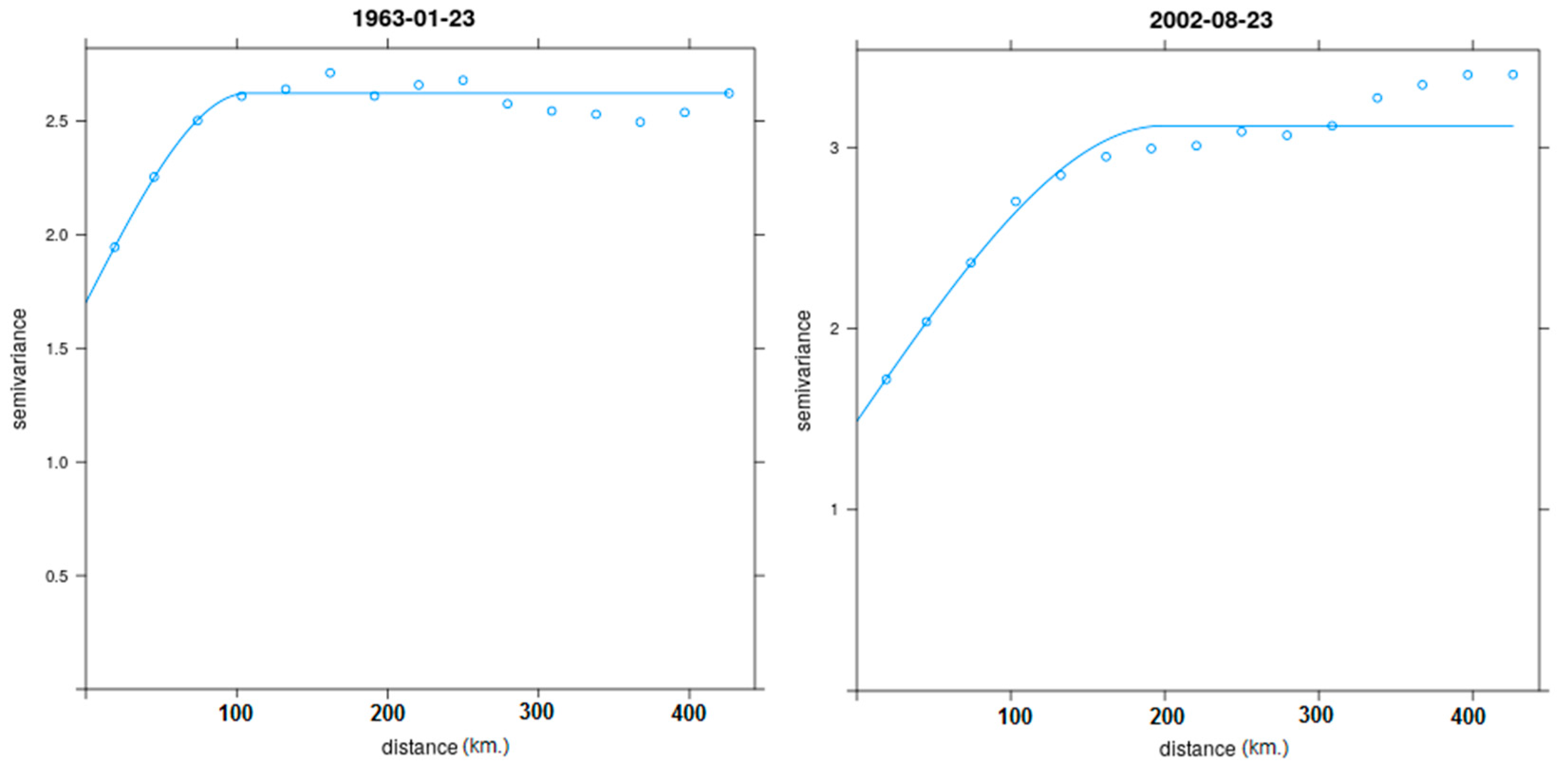
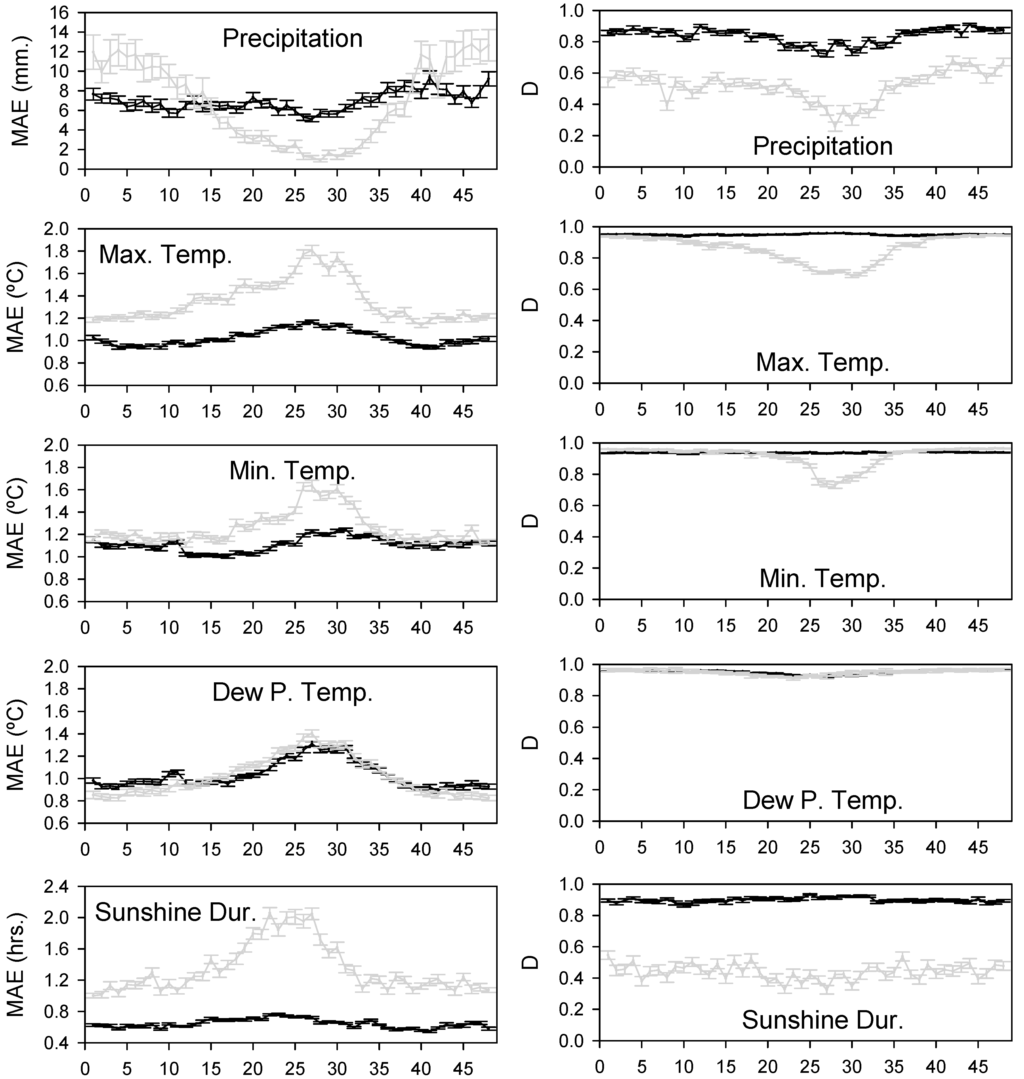
3.2. Climate Gridding and Evaluation

Using the available meteorological series, a weekly gridded dataset of the five variables was created at a spatial resolution of 1.1 × 1.1 km to match with other satellite products such as those derived from the NOAA-AVHRR satellites. These grids were used as inputs to calculate the drought indices. For this purpose, a universal kriging method was applied [26,27], with the geographic latitude, longitude, and elevation of each grid cell being considered auxiliary variables. Two zones were considered for the interpolation: (i) the Spanish Peninsular area and the Balearic Islands (PSBI); and (ii) the Canary Islands (CI). A maximum of 50 neighboring observatories and a range of 250 km were considered in obtaining weights for the interpolations and spherical semivariograms with nugget effect. Figure 2 shows the example of spherical semivariograms used to interpolate two maximum temperature layers.

The grid layers were validated using a jackknife resampling procedure. This was based on withholding single observatories in turn from the network, making estimates based on interpolation from the remaining observatories, and calculating the difference between the predicted and observed values for each observatory that was withheld [28]. This approach was repeated each week as many times as available observatories of each climate variable so thousands of interpolations were applied for the validation of each variable. For each gridded layer for the six variables analyzed, the mean absolute error (MAE) and the agreement Index D were calculated. Index D [29] is a relative and bounded measure of model validity, and it scales with the magnitude of the variables, retaining mean information and not amplifying outliers. A D value = 1 corresponds to a perfect match between estimates and the observed data. Figure 3 shows the mean and standard error of the mean for MAE and D statistics from the weekly gridded data for the six meteorological variables. Statistics are provided independently for the PSBI and CI zones. As expected, given the availability of data and relief complexity, the statistics were much better for the PSBI zone than for the CI zone. For the PSBI zone, with the exception of wind speed the D values were very high and ranged from 0.9 to 1. In addition, no seasonal patterns were evident in the D statistic, indicating that the quality of the gridded data was independent of the season of the year. For the CI zone, the agreement between the observed and predicted data was lower, and some seasonal patterns were evident, mainly for precipitation and temperature data.

3.3. Calculation of the Reference Evapotranspiration

The reference evapotranspiration (ETo) was obtained using the FAO-56 Penman-Monteith (PM) equation [30]. The PM method can be used globally, and has been widely verified based on lysimeter data from diverse climate regions [31,32]. The reference surface for calculations is a hypothetical crop (assumed height: 0.12 m; surface resistance: 70 s m⁻¹; albedo: 0.23) that has evaporation similar to that of an extended surface of green grass of uniform height that is actively growing and adequately watered. ETo can be calculated from measurements of the weekly averages for five meteorological parameters: maximum temperature, minimum temperature, dew point temperature (which determines the vapor pressure deficit), wind speed at a height of 2 m, and daily sunshine duration (following [30]). The ETo weekly gridded data were obtained from the grids of the various meteorological variables described above.

3.4. Drought Index Calculation

Using the gridded data for precipitation and ETo, the seven drought indices were calculated. The four self-calibrated Palmer drought indices were calculated according to [33]. For this purpose, we used the available code at http://greenleaf.unl.edu/, which was modified to include the ETo calculated using the PM equation, and to be run directly in R. The SPI was calculated following the recommendations of the World Meteorological Organization [34], using a two-parameter gamma distribution. The SPEI was calculated using a three-parameter log-logistic distribution using non-biased Probabilistic Weighted Moments (PWMs) to calculate the parameters (see details in [13,35]. The SPDI was obtained following [36], but we used the three-parameter log-logistic distribution instead of the recommended General Extreme Value distribution to avoid problems with extreme values, and, in some cases, inability to perform the calculation (see [37]). To calculate the SPEI, SPI, and SPDI, we used the SPEI R library [35].

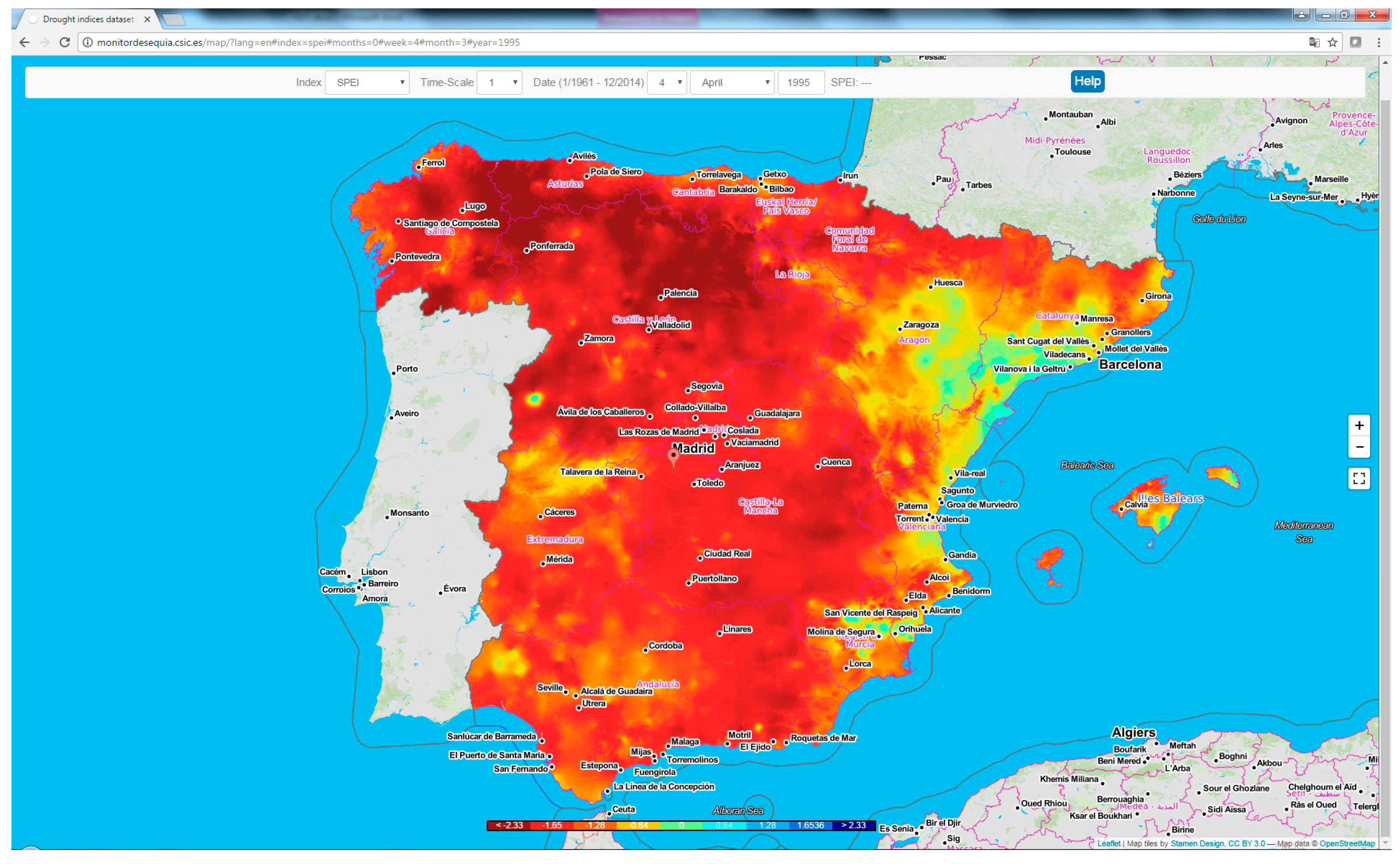
4. Data Use and Application

Gridded drought indices are widely used for climatological analyses of droughts. In particular, several recent studies have used gridded drought indices at the global scale to determine the recent evolution of climate droughts and the impacts of climate change on drought severity [38,39]. The availability of a comprehensive drought dataset for Spain will be useful in investigations of several climate issues related to the spatial and temporal variability of droughts, and also to develop drought catalogues that consider the severity, duration, and spatial extent of drought events (http://droughtatlas.unl.edu/). Drought indices have also been widely used to determine the magnitude of droughts [40], and to create probability maps of drought duration and severity [41,42], which are useful resources for drought management. These analyses could be applied in Spain using the drought index dataset described in this study.

Gridded drought indices have been widely used in a variety of systems to identify drought impacts, including tree morbidity and mortality at various spatial scales [43,44], crop yield reductions and crop failures [45], forest fires [46,47], and decreased vegetation activity [48,49]. The developed dataset will also be widely useful for the assessment of land degradation. Although a number of studies have addressed land degradation in Spain [50,51,52], and the connection between land degradation and drought variability [53], they have all been based on low resolution data. The current drought index dataset has been created at a very high spatial resolution (1.1 km), which matches with current vegetation products available from earth observation satellites including MODIS and NOAA-AVHRR, and this will facilitate spatial and temporal assessment of the climate drivers of land degradation in Spain, and improvement of the surveillance systems to prevent land degradation [54].

5. Dataset Availability

The drought indices dataset is available in a map visualization tool (http://monitordesequia.csic.es) in which the spatial drought conditions from 1961 to 2014 can be visualized. The web visualization tool uses standard tools: HTML, CSS, Javascript and PHP. It uses jQuery, a Javascript library, to simplify the use of AJAX and the DOM management; Leaflet, a library for map visualization; and Dygraphs, a library for graph visualization. This tool enables zooming and identification of single grid points in the map. Once a grid point is selected, a time series for the selected drought index can be visualized. It is possible to move throughout the time series to identify the drought index values for each weekly time step. The time series can be modified for each point, enabling selection of other drought indices and time scales. Time series of drought indices for the selected grid points can be downloaded as plain text in *.csv format. Moreover, the entire dataset for each drought index and time scale (from 1 to 48 months) can be independently downloaded in netCDF4 format for each spatial domain (PSBI and CI). All the information available at the website is provided in Spanish and English. Figure 4 shows a general overview of the web spatial tool, and where the dataset can be visualized and downloaded.

References

1. Lal, R. Soil degradation by erosion. Land Degrad. Dev. 2001, 12, 519–539. [Google Scholar] [CrossRef]
2. Nicholson, S.E.; Tucker, C.J.; Ba, M.B. Desertification, drought and surface vegetation: An example from the west African Sahel. Bull. Am. Meteorol. Soc. 1998, 79, 815–829. [Google Scholar] [CrossRef]
3. Pickup, G. Desertification and climate change—The Australian perspective. Clim. Res. 1998, 11, 51–63. [Google Scholar] [CrossRef]
4. Wilhite, D.A. Drought as a natural hazard: Concepts and definitions. In Drought: A Global Assessment; Routledge: Abingdon, UK, 2000; Volume 1, pp. 3–18. [Google Scholar]
5. Cook, B.I.; Miller, R.L.; Seager, R. Amplification of the North American "Dust Bowl" drought through human-induced land degradation. Proc. Natl. Acad. Sci. USA 2009, 106, 4997–5001. [Google Scholar] [CrossRef] [PubMed]
6. Vicente-Serrano, S.M.; Zouber, A.; Lasanta, T.; Pueyo, Y. Dryness is accelerating degradation of vulnerable shrublands in semiarid Mediterranean environments. Ecol. Monogr. 2012, 82, 407–428. [Google Scholar] [CrossRef]
7. Wilhite, D.A. Drought Assessment, Management and Planning: Theory and Case Studies; Kluwer Academic Publishers: Boston, MA, USA, 1993. [Google Scholar]
8. Svoboda, M.; LeCompte, D.; Hayes, M.; Heim, R.; Gleason, K.; Angel, J.; Rippey, B.; Tinker, R.; Palecki, M.; Stooksbury, D.; et al. The drought monitor. Bull. Am. Meteorol. Soc. 2002, 83, 1181–1190. [Google Scholar]
9. Heim, R.R., Jr. A review of twentieth-century drought indices used in the United States. Bull. Am. Meteorol. Soc. 2002, 83, 1149–1165. [Google Scholar]
10. Mishra, A.K.; Singh, V.P. A review of drought concepts. J. Hydrol. 2010, 391, 202–216. [Google Scholar] [CrossRef]
11. Zargar, A.; Sadiq, R.; Naser, B.; Khan, F.I. A review of drought indices. Environ. Rev. 2011, 19, 333–349. [Google Scholar] [CrossRef]
12. McKee, T.B.N.; Doesken, J.; Kleist, J. The relationship of drought frequency and duration to time scales. In Proceedings of the 8th Conference on Applied Climatology, Anaheim, CA, USA, 17–22 January 1993; pp. 179–183. [Google Scholar]
13. Vicente-Serrano, S.M.; Beguería, S.; López-Moreno, J.I. A Multi-scalar drought index sensitive to global warming: The Standardized Precipitation Evapotranspiration Index—SPEI. J. Clim. 2010, 23, 1696–1718. [Google Scholar] [CrossRef]
14. Vicente-Serrano, S.M.; Cuadrat, J.M. North Atlantic Oscillation control of droughts in Northeast of Spain: Evaluation since A.D. 1600. Clim. Change 2007, 85, 357–379. [Google Scholar] [CrossRef]
15. Domínguez-Castro, F.; Ribera, P.; García-Herrera, R.; Cuadrat, J.M.; Moreno, J.M. Assessing extreme droughts in Spain during 1750–1850 from rogation ceremonies. Clim. Past 2012, 8, 705–722. [Google Scholar] [CrossRef]
16. Vicente-Serrano, S.M. Spatial and temporal analysis of droughts in the Iberian Peninsula (1910–2000). Hydrol. Sci. J. 2006, 51, 83–97. [Google Scholar] [CrossRef]
17. Vicente-Serrano, S.M. Spatial and temporal evolution of precipitation droughts in Spain in the last century. In Adverse Weather in Spain; Martínez, C.C.-L., Rodríguez, F.V., Eds.; WCRP Spanish Committee: Madrid, Spain, 2013; pp. 283–296. [Google Scholar]
18. Maia, R.; Vicente-Serrano, S.M. Drought Planning and Management in the Iberian Peninsula. In Drought and Water Crises: Science, Technology and Management Issues; Wilhite, D., Pulwarty, R.S., Eds.; CRC: Boca Raton, FL, USA, 2017. [Google Scholar]
19. Lorenzo-Lacruz, J.; Vicente-Serrano, S.M.; González-Hidalgo, J.C.; López-Moreno, J.I.; Cortesi, N. Hydrological drought response to meteorological drought at various time scales in the Iberian Peninsula. Clim. Res. 2013, 58, 117–131. [Google Scholar] [CrossRef]
20. Carnicer, J.; Coll, M.; Ninyerola, M.; Pons, X.; Sánchez, G.; Peñuelas, J. Widespread crown condition decline, food web disruption, and amplified tree mortality with increased climate change type drought. Proc. Natl. Acad. Sci. USA 2011, 108, 1474–1478. [Google Scholar] [CrossRef] [PubMed]
21. Camarero, J.J.; Gazol, A.; Sangüesa-Barreda, G.; Oliva, J.; Vicente-Serrano, S.M. To die or not to die: Early warnings of tree dieback in response to a severe drought. J. Ecol. 2015, 103, 44–57. [Google Scholar] [CrossRef]
22. Vicente-Serrano, S.M. Evaluating the Impact of Drought Using Remote Sensing In a Mediterranean, Semi-Arid Region. Nat. Hazard. 2007, 40, 173–208. [Google Scholar] [CrossRef]
23. Páscoa, P.; Gouveia, C.M.; Russo, A.; Trigo, R.M. The role of drought on wheat yield interannual variability in the Iberian Peninsula from 1929 to 2012. Int. J. Biometeorol. 2017, 61, 439–451. [Google Scholar] [CrossRef] [PubMed]
24. Tomas-Burguera, M.; Jimenez, A.; Luna, M.Y.; Morata, A.; Vicente-Serrano, S.M.; González-Hidalgo, J.C.; Beguería, S. Control de Calidad de Siete Variables del Banco Nacional de Datos de AEMET; Olcina Cantos, J., Rico Amorós, A.M., Moltó Mantero, E., Eds.; Universidad de Alicante: Alicante, Spain, 2016; pp. 407–415. [Google Scholar]
25. Alexandersson, H. A homogeneity test applied to precipitation data. J. Climatol. 1986, 6, 661–675. [Google Scholar] [CrossRef]
26. Borrough, P.A.; McDonnell, R.A. Principles of Geographical Information Systems; Oxford University Press: Oxford, UK, 1998. [Google Scholar]
27. Pebesma, E.J. Multivariable geostatistics in S: The gstat package. Comput. Geosci. 2004, 30, 683–691. [Google Scholar] [CrossRef]
28. Phillips, D.L.; Dolph, J.; Marks, D. A comparison of geostatistical procedures for spatial analysis of precipitation in mountainous terrain. Agric. Meteorol. 1992, 58, 119–141. [Google Scholar] [CrossRef]
29. Willmott, C.J. Some comments on the evaluation of model performance. Bull. Am. Meteorol. Soc. 1982, 63, 1309–1313. [Google Scholar] [CrossRef]
30. Allen, R.G.; Pereira, L.S.; Raes, D.; Smith, M. Crop evapotranspiration: Guidelines for computing crop water requirements. FAO 1998, 300, D05109. [Google Scholar]
31. Itenfisu, D.; Elliott, R. L.; Allen, R.G.; Walter, I.A. Comparison of Reference Evapotranspiration Calculations across a Range of Climates. In Proceedings of the 4th National Irrigation Symposium, Phoenix, AZ, USA, 14–16 November 2000; pp. 216–227. [Google Scholar]
32. López-Urrea, R.; Martín de Santa Olalla, F.; Fabeiro, C.; Moratalla, A. Testing evapotranspiration equations using lysimeter observations in a semiarid climate. Agric. Water Manag. 2006, 85, 15–26. [Google Scholar] [CrossRef]
33. Wells, N.; Goddard, S.; Hayes, M.J. A self-calibrating Palmer drought severity index. J. Clim. 2004, 17, 2335–2351. [Google Scholar] [CrossRef]
34. World Meteorological Organization. Standardized Precipitation Index User Guide. Available online: http://www.wamis.org/agm/pubs/SPI/WMO_1090_EN.pdf (accessed on 27 June 2017).
35. Beguería, S.; Vicente-Serrano, S.M.; Reig, F.; Latorre, B. Standardized Precipitation Evapotranspiration Index (SPEI) revisited: Parameter fitting, evapotranspiration models, kernel weighting, tools, datasets and drought monitoring. Int. J. Climatol. 2014, 34, 3001–3023. [Google Scholar] [CrossRef]
36. Ma, M.; Ren, L.; Yuan, F.; Jiang, S.; Liu, Y.; Kong, H.; Gong, L. A new standardized Palmer drought index for hydro-meteorological use. Hydrol. Process. 2014, 28, 5645–5661. [Google Scholar] [CrossRef]
37. Vicente-Serrano, S.M.; Beguería, S. Comment on “Candidate Distributions for Climatological Drought Indices (SPI and SPEI)” by James H. Stagge et al. Int. J. Clim. 2016, 36, 2120–2131. [Google Scholar] [CrossRef]
38. Sheffield, J.; Wood, E.J.; Roderick, M.L. Little change in global drought over the past 60 years. Nature 2012, 491, 435–438. [Google Scholar] [CrossRef] [PubMed]
39. Dai, A. Increasing drought under global warming in observations and models. Nat. Clim. Change 2013, 3, 52–58. [Google Scholar] [CrossRef]
40. Dracup, J.A.; Lee, K.S.; Paulson, E.G. On the Statistical Characteristics of Drought Events. Water Resour. Res. 1980, 16, 289–296. [Google Scholar] [CrossRef]
41. Santos, J.F.; Portela, M.M.; Pulido-Calvo, I. Regional Frequency Analysis of Droughts in Portugal. Water Resour. Manag. 2011, 25, 3537–3558. [Google Scholar] [CrossRef]
42. Vicente-Serrano, S.M.; Beguería, S.; Gimeno, L.; Eklundh, L.; Giuliani, G.; Weston, D.; El Kenawy, A.; López-Moreno, J.I.; Nieto, R.; Ayenew, T.; et al. Challenges for drought mitigation in Africa: The potential use of geospatial data and drought information systems. Appl. Geogr. 2012, 34, 471–486. [Google Scholar] [CrossRef]
43. Merlin, M.; Perot, T.; Perret, S.; Korboulewsky, N.; Vallet, P. Effects of stand composition and tree size on resistance and resilience to drought in sessile oak and Scots pine. For. Ecol. Manag. 2015, 339, 22–33. [Google Scholar] [CrossRef]
44. Greenwood, S.; Ruiz-Benito, P.; Martínez-Vilalta, J.; Lloret, F.; Kitzberger, T.; Allen, C.D.; Fensham, R.; Laughlin, D.C.; Kattge, J.; Bönisch, G.; et al. Tree mortality across biomes is promoted by drought intensity, lower wood density and higher specific leaf area. Ecol. Lett. 2017, 20, 539–553. [Google Scholar] [CrossRef] [PubMed]
45. Zipper, S.C.; Qiu, J.; Kucharik, C.J. Drought effects on US maize and soybean production: Spatiotemporal patterns and historical changes. Environ. Res. Lett. 2016, 11, 094021. [Google Scholar] [CrossRef]
46. Turco, M.; Levin, N.; Tessler, N.; Saaroni, H. Recent changes and relations among drought, vegetation and wildfires in the Eastern Mediterranean: The case of Israel. Glob. Planet. Change 2017, 151, 28–35. [Google Scholar] [CrossRef]
47. Russo, A.; Gouveia, C.M.; Páscoa, P.; DaCamara, C.C.; Sousa, P.M.; Trigo, R.M. Assessing the role of drought events on wildfires in the Iberian Peninsula. Agric. For. Meteorol. 2017, 237, 50–59. [Google Scholar] [CrossRef]
48. Ivits, E.; Horion, S.; Fensholt, R.; Cherlet, M. Drought footprint on European ecosystems between 1999 and 2010 assessed by remotely sensed vegetation phenology and productivity. Glob. Change Biol. 2014, 20, 581–593. [Google Scholar] [CrossRef] [PubMed]
49. Vicente-Serrano, S.M.; Cabello, D.; Tomás-Burguera, M.; Martín-Hernández, N.; Beguería, S.; Azorin-Molina, C.; Kenawy, K.E. Drought variability and land degradation in semiarid regions: Assessment using remote sensing data and drought indices (1982–2011). Remote Sens. 2015, 7, 4391–4423. [Google Scholar] [CrossRef]
50. Symeonakis, E.; Calvo-Cases, A.; Arnau-Rosalen, E. Land use change and land degradation in southeastern Mediterranean Spain. Environ. Manag. 2007, 40, 80–94. [Google Scholar] [CrossRef] [PubMed]
51. Contador, J.F.L.; Schnabel, S.; Gómez Gutiérrez, A.; Pulido Fernández, M. Mapping sensitivity to land degradation in Extremadura, SW Spain. Land Degrad. Dev. 2009, 20, 129–144. [Google Scholar] [CrossRef]
52. Del Barrio, G.; Puigdefabregas, J.; Sanjuan, M.E.; Stellmes, M.; Ruiz, A. Assessment and monitoring of land condition in the Iberian Peninsula, 1989–2000. Remote Sens. Environ. 2010, 114, 1817–1832. [Google Scholar] [CrossRef]
53. Gouveia, C.M.; Páscoa, P.; Russo, A.; Trigo, R.M. Land degradation trend assessment over Iberia during 1982–2012. Cuad. Investig. Geogr. 2016, 42, 89–112. [Google Scholar] [CrossRef]
54. Martínez-Valderrama, J.; Ibáñez, J.; Del Barrio, G.; Sanjuán, M.E.; Alcalá, F.J.; Martínez-Vicente, S.; Ruiz, A.; Puigdefábregas, J. Present and future of desertification in Spain: Implementation of a surveillance system to prevent land degradation. Sci. Total Environ. 2016, 563, 169–178. [Google Scholar] [CrossRef] [PubMed]
Figure 1. Spatial distribution of the meteorological stations for the dataset variables. Gray: original stations. Black: definitive complete and homogeneous observatories.
Data 02 00022 g001
Figure 2. Examples of spherical semivariograms used to develop the weekly maximum temperature gridded layers.
Data 02 00022 g002
Figure 3. Mean and standard error of the mean for MAE and D for the six meteorological variables. Black: Peninsular Spain and the Balearic Islands. Gray: Canary Islands. All the variables are calculated in the original units per week.
Data 02 00022 g003aData 02 00022 g003b
Figure 4. Web spatial tool showing the data to be visualized and downloaded.
Data 02 00022 g004