Abstract
Robust credit risk prediction in emerging economies increasingly demands the integration of external factors (EFs) beyond borrowers’ control. This study introduces a scenario-based methodology to incorporate EF—namely COVID-19 severity (mortality and confirmed cases), climate anomalies (temperature deviations, weather-induced road blockages), and social unrest—into machine learning (ML) models for credit delinquency prediction. The approach is grounded in a CRISP-DM framework, combining stationarity testing (Dickey–Fuller), causality analysis (Granger), and post hoc explainability (SHAP, LIME), along with performance evaluation via AUC, ACC, KS, and F1 metrics. The empirical analysis uses nearly 8.2 million records compiled from multiple sources, including 367,000 credit operations granted to individuals and microbusiness owners by a regulated Peruvian financial institution (FMOD) between January 2020 and September 2023. These data also include time series of delinquency by economic activity, external factor indicators (e.g., mortality, climate disruptions, and protest events), and their dynamic interactions assessed through Granger causality to evaluate both the intensity and propagation of external shocks. The results confirm that EF inclusion significantly enhances model performance and robustness. Time-lagged mortality (COVID MOV) emerges as the most powerful single predictor of delinquency, while compound crises (climate and unrest) further intensify default risk—particularly in portfolios without public support. Among the evaluated models, CNN and XGB consistently demonstrate superior adaptability, defined as their ability to maintain strong predictive performance across diverse stress scenarios—including pandemic, climate, and unrest contexts—and to dynamically adjust to varying input distributions and portfolio conditions. Post hoc analyses reveal that EF effects dynamically interact with borrower income, indebtedness, and behavioral traits. This study provides a scalable, explainable framework for integrating systemic shocks into credit risk modeling. The findings contribute to more informed, adaptive, and transparent lending decisions in volatile economic contexts, relevant to financial institutions, regulators, and risk practitioners in emerging markets.
1. Introduction
Currently, artificial intelligence (AI), machine learning (ML), and process digitization are fundamental elements of daily life. This trend began in the 1990s with the global expansion of the Internet [1] and notably intensified during the COVID-19 pandemic [2]. Simultaneously, the increase in the use of online credit has generated large volumes of data [3], leading the financial industry to the imperative need to develop advanced technological tools for risk prediction and effective uncertainty management [4] that include exogenous variables in the process [5]. Presently, scoring models and machine learning techniques are common for risk prediction, applying innovations based on exhaustive data analysis, data-driven innovation (DDI) [6], and the big data paradigm—characterized by the use of massive, high-dimensional, and heterogeneous datasets for predictive modeling and decision-making [7].
In the context of rising demand, credit risk levels show a significant increase [8,9]. Despite the growing integration of DDI and ML in the financial sector, substantial challenges persist, leaving numerous applications unexplored. The application of ML techniques during unpredictable events, such as the 2008 housing crisis [2,10], the COVID-19 pandemic [11], and the impacts of climate change [12], has exposed critical limitations in risk assessment methodologies and revealed considerable uncertainties in their outputs [2,13,14,15]. These challenges underscore the need to examine the influence of external factors (EF) on the accuracy and robustness of ML models in credit risk evaluation [6,16], particularly concerning the inclusion of sequential or time-series data, which are commonly encountered in credit risk scenarios [17]. Moreover, these issues emphasize the need to ensure explainability in ML-driven predictions [18], both to facilitate informed decision-making by stakeholders and to maintain transparency for all parties involved [19].
The main objective of this article is to address the integration of variables sensitive to external risk factors into machine learning models for credit risk assessment, a critical yet insufficiently explored topic in the academic context. Peru, as a case study, represents a particularly relevant scenario: it was the country with the highest COVID-19 death rate per 100,000 inhabitants during the pandemic [20]; it faced the periodic and devastating effects of the El Niño phenomenon [12]; and it experienced intense social unrest following the attempted coup in December 2022 [21]. These events have directly impacted the microcredit market by targeting small businesses, a sector highly vulnerable to risk volatility [12].
While the influence of external factors—such as macroeconomic variables and pandemic-related disruptions—on credit risk has been the subject of substantial academic research, few studies have explored the simultaneous integration of multiple external shocks (pandemics, climate anomalies, and social unrest) into ML-based credit risk models, especially in emerging economies such as Peru. This study addresses that gap, offering valuable insights into the applicability and extrapolation of multifactor risk models in vulnerable financial systems [12]. To this end, EF-related variables are integrated into credit risk models through causality and stationarity tests [22]. These variables are derived from public time-series data and combined with proprietary credit data provided by a regulated Peruvian financial institution—hereafter referred to as FMOD—used under a confidentiality agreement. This strategy not only enhances the predictive power of ML models but also establishes a replicable methodology for integrating diverse EF indicators into future risk prediction studies.
The FMOD dataset plays a pivotal role in this study. It incorporates a unique variable that identifies loans supported by government intervention during periods influenced by EF, such as climate change, social unrest, and the COVID-19 pandemic. This variable allows for the detection and detailed analysis of the potential biases introduced by mitigation programs designed to address economic disruptions. By explicitly accounting for these interventions, the FMOD dataset provides a nuanced understanding of how state-led programs shape credit risk dynamics and borrower behavior under varying external conditions.
Moreover, the FMOD dataset includes monthly updated records of delinquency days, enabling granular analysis across distinct periods. This temporal precision facilitates an in-depth exploration of the interplay between EF and default patterns, thus enhancing the methodological rigor of credit risk assessment. By integrating time-series data with real-world financial indicators, the FMOD dataset offers a robust and replicable framework for evaluating the influence of EF and government programs on financial stability and credit behavior in emerging markets.
Finally, this study evaluates the impact of EF on the predictive accuracy and explainability of ML models. Particular attention is paid to identifying the most influential factors when incorporating external variables into predictive frameworks. By addressing these challenges, this research not only fills a critical gap in the existing literature but also advances the understanding of the effects of EF on credit risk in emerging economies. This contributes actionable insights for policymakers and financial institutions aiming to enhance resilience in volatile economic environments.
2. Related Work
Credit risk, an inherent component of financial activities, arises when borrowers fail to meet their credit obligations, typically due to inability rather than unwillingness to pay [23]. This form of credit deterioration is strongly associated with demographic and macroeconomic variables—such as household income and employment—which are, in turn, sensitive to external systemic shocks [9,23]. Enhancing the explainability of these complex relationships is essential to support data-driven decision-making for policymakers, financial institutions, and affected communities.
The recent literature has increasingly focused on the role of exogenous compound shocks—namely, pandemics, climate change, and social unrest—as emerging sources of credit instability. These phenomena often co-occur and interact in nonlinear ways, producing cascading effects on borrower behavior, portfolio quality, and systemic financial resilience.
- COVID-19 and Credit Risk: The COVID-19 pandemic exposed critical limitations in traditional credit risk models. Government interventions—such as moratoriums, liquidity injections, and public credit guarantees—generated structural breaks in borrower behavior, which challenged the assumptions of pre-pandemic models and led to inaccurate estimations of default risk [11]. These disruptions particularly affected financially vulnerable groups as noted in recent empirical analyses [24].Several studies have highlighted the necessity of using adaptive, data-driven approaches—such as deep learning and regularized regression models—to handle the nonlinearity and volatility introduced by systemic shocks [25,26,27]. In the Peruvian context, unemployment shocks and loan restructuring policies were found to be key drivers of delinquency in consumer and microfinance credit portfolios during the pandemic period [28,29]. Evidence also suggests that regularized machine learning models, including Lasso and Ridge regression, offer robust predictive performance under uncertainty, particularly in large-scale government programs such as “Reactiva Perú” [27].
- Climate-Related Risks: Climate change poses both physical risks (e.g., floods and droughts) and transition risks (e.g., carbon pricing and regulatory shifts), each with distinct implications for credit stability. Physical hazards can disrupt supply chains, damage infrastructure, and reduce household and firm-level repayment capacity [30], while transition risks expose high-emission sectors to market penalties and regulatory uncertainty [31,32].Empirical evidence shows that extreme climate events elevate loan impairment rates and increase provisioning requirements, particularly for microfinance institutions operating in vulnerable regions [12]. These dynamics underscore the urgency of integrating climate stress testing, early-warning systems, and network-aware modeling into credit risk frameworks [33,34].This study [35] analyzes the interaction between macroeconomic shocks and climate-driven economic pressures within the Peruvian context, using a vector autoregression (VAR) model with national time-series data. Their findings suggest that expansionary monetary policies during periods of climate-related stress may inadvertently elevate the credit risk of microfinance portfolios. This reinforces the need to develop predictive frameworks that account for both environmental and policy-related drivers of credit instability in emerging economies.
- Social Unrest and Political Instability: Social unrest—often triggered by inequality, political crises, or economic shocks—can significantly amplify credit risk by disrupting income flows, consumption patterns, and investor confidence. Empirical evidence from Chile shows that the 2019 protests led to a measurable increase in household default probability, with partial mitigation through pandemic-era relief programs [36]. Similarly, civil unrest has been shown to induce volatility in financial markets, exemplified by reverse herding behaviors among investors [37], and to influence regulatory responses such as foreclosure bans, which may inadvertently elevate long-term credit risk [38]. In the Middle East and North Africa (MENA) region, waves of political instability have prompted structural reforms such as bank privatization, producing mixed outcomes in terms of credit risk and financial system resilience [39].While regional and global analyses are increasingly available, country-level studies for Peru remain scarce. However, recent academic research suggests that social and health crises in Peru prompted a behavioral shift among microentrepreneurs, particularly those in lower-poverty districts, who increasingly substituted personal loans with government-backed business credit during times of elevated uncertainty. This substitution pattern reflects a form of borrower adaptation and highlights the indirect impact of public policy interventions—such as state guarantee programs—on the structure and resilience of credit portfolios in emerging markets [29].
- Compound External Shocks: An emerging body of research highlights that the simultaneous occurrence of exogenous stressors—such as pandemics, climate anomalies, and social unrest—can generate nonlinear, systemic risks that conventional credit risk models are ill-equipped to anticipate [40]. These compound shocks interact across temporal and spatial dimensions, producing cascading effects on borrower behavior, institutional solvency, and portfolio stability. Moreover, societal vulnerabilities such as institutional fragility, inequality, and economic informality intensify the transmission channels and feedback loops of these risks, particularly in emerging economies.To address this complexity, researchers have proposed integrated modeling frameworks that incorporate early-warning signals, tipping points, and network-aware propagation mechanisms spanning environmental, economic, and political domains [40]. These multidimensional approaches are considered essential for the development of next-generation credit risk systems capable of operating under deep systemic uncertainty.In the Peruvian context, recent analyses emphasize the need for credit scoring systems to account for borrower heterogeneity under compound volatility conditions [41]. Empirical studies support the use of hybrid models that integrate Explainable Artificial Intelligence (XAI) techniques—such as SHapley Additive Explanations (SHAP) and Local Interpretable Model-Agnostic Explanations (LIME)—into traditional risk evaluation processes, thereby enhancing model transparency and predictive performance in highly unstable environments [23]. These insights reinforce the urgency of designing robust, adaptive credit assessment tools tailored to complex and evolving risk landscapes.
Despite the growing body of work on machine learning applications for credit scoring in Peru, most studies focus on conventional financial variables without incorporating external systemic stressors. Prior research has evaluated multiple machine learning algorithms for microcredit assessment in rural areas but typically omits exogenous factors such as pandemic shocks or climate anomalies [42]. This reveals a gap in studies that simultaneously integrate multiple external variables into ML-based credit risk models, particularly within the Peruvian financial system.
The present study addresses this limitation by incorporating time-series-based exogenous indicators—including COVID-19 deaths, temperature anomalies, and climate-induced road blockades—into a wide range of ML models. We assess their influence on both predictive accuracy and model interpretability.
3. Materials and Methods
3.1. Research Questions and Data Description
Based on this assessment, this article poses the research questions outlined in Table 1, centering on the interplay between external factors and credit risk assessment. Particular emphasis is placed on the importance of explainability in ML-driven models, as understanding how EF impacts credit risk is critical for decision-making and actionable insights.

Table 1.
Research questions.
To explore these relationships, a study focusing on Peru from January 2020 to September 2023 was conducted. The analysis was based on a comprehensive dataset comprising nearly 8.2 million records, as summarized in Table 2. This dataset integrates diverse EF, such as COVID-19 positive cases and deaths, road blockages, and temperature anomalies, along with financial delinquency (see Table 3) and credit activity data (see Table 4), ensuring a multifaceted approach to understanding credit risk dynamics under external influences.
Table 2.
Datasets.
Table 3.
Description of variables in the time-series dataset on credit delinquency by economic activity.
Table 4.
Summary of variables used in the modeling experiments.
Figure 1 illustrates the trends of various external factors, including COVID-19 cases (positive and dead), social unrest, road blockages due to social unrest and weather, and temperature anomalies. Peaks in certain factors, such as COVID-19 cases and social unrest, were visible during specific periods, indicating their significant occurrence and potential impact on other events or systems.
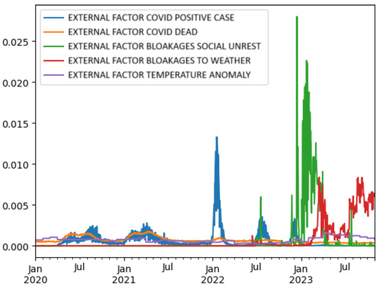
Figure 1.
Time series visualization of external factors from January 2020 to September 2023. The plot includes normalized series (min–max scaled) for external factors such as COVID-19 confirmed cases, COVID-19 deaths, protest-related road blockages, weather-induced road blockages, and temperature anomalies. The y-axis ranges from 0 to 1, representing relative intensity over time for each factor. This normalization facilitates the comparison of dynamic patterns across factors with different units and magnitudes.
The main features of the credit dataset provided by FMOD are summarized in Table 5. This summary complements the structural descriptions in Table 3 and Table 4.
Table 5.
Descriptive statistics of the credit dataset used for modeling (FMOD).
Table 3 presents the structure of the time-series dataset used to analyze credit delinquency patterns across economic activities. Each row corresponds to an aggregated daily observation, capturing both the average and maximum number of overdue days among loans, grouped by income source, loan purpose, and economic sector. These variables are essential for modeling how different segments of the economy responded to external shocks over time.
By combining these features, the study constructed temporal indicators of financial stress, which were then aligned with a time series of external factors (e.g., COVID-19 indicators and climate anomalies). This temporal alignment enabled the application of causality analyses—such as Granger causality tests—and enhanced the interpretability of the model’s behavior under compound external disruptions.
This approach not only evaluates the predictive accuracy of machine learning models but also examines their capacity to provide transparent explanations for the relationships uncovered, ensuring their practical relevance for decision-making in volatile and complex environments.
Additionally, Table 4 summarizes the set of features used in the individual-level credit risk modeling. These include socio-demographic variables, financial indicators, and normalized business metrics. Each row corresponds to a credit evaluated during the study period, enriched with external factor indicators to support scenario-based experimentation.
Among the set of features, two representative variables were constructed with monthly frequency for this study: ‘DelinquencyDays_MMYYYY’, which captures the number of overdue days per month, and ‘ExternalFactorImpact_MMYYYY’, which flags the presence of external stressors—such as COVID-19, climate anomalies, or social unrest—during the same period. This temporal alignment enabled a dynamic analysis of credit behavior under external disruptions, strengthening both the predictive modeling and the interpretability of the results.
3.2. Cross-Industry Standard Process for Data Mining
To evaluate the influence of EF on credit risk, we adopt the Cross-Industry Standard Process for Data Mining (CRISP-DM), a widely used framework that structures data mining projects into six iterative stages: Business Understanding, Data Understanding, Data Preparation, Modeling, Evaluation, and Deployment [43]. This methodological foundation provides a robust and flexible structure for guiding machine learning workflows across domains, and has also been successfully applied in prior studies analyzing external factors during crisis scenarios [44,45].
In the context of this study, the application of CRISP-DM allowed us to address two specific challenges associated with modeling credit risk under compound external shocks. First, during the Data Understanding and Preparation phases, the incorporation of exogenous time-series variables—such as pandemic indicators, climate anomalies, and social unrest—required additional preprocessing steps, including stationarity testing, temporal alignment, and Granger causality analysis. Second, during the Modeling and Evaluation phases, we conducted comparative experiments across multiple scenarios (with and without EF), enabling us to assess the marginal contribution and explanatory power of these external variables under volatile conditions.
As illustrated in Figure 2, the CRISP-DM framework provided a structured and iterative foundation for organizing each phase of the experiment. The process began with Business and Data Understanding, which guided the initial dataset exploration and external factor characterization. During Data Preparation, we performed normalization, standardization, and the integration of exogenous time-series variables. This integration was based on a monthly alignment strategy.
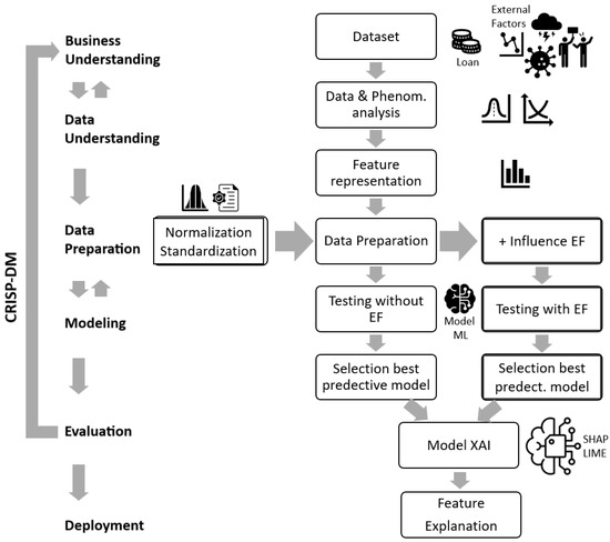
Figure 2.
CRISP-DM framework applied to EF-driven credit risk modeling. This diagram illustrates how the CRISP-DM phases structure the experimental workflow, from data understanding and preparation—including the monthly alignment and integration of exogenous time-series variables—to scenario-based modeling (with and without external factors) and the use of explainable AI techniques (SHAP and LIME) during evaluation. The variables DelinquencyDays_MMYYYY and ExternalFactorImpact_MMYYYY are constructed to support a time-aware analysis of credit behavior and its relationship to validated external shocks across economic sectors.
Importantly, the ‘ExternalFactorImpact_MMYYYY’ variable was not assigned uniformly across the dataset. Instead, it was derived by evaluating the declared economic activity of each credit and determining whether that activity exhibited a statistically significant relationship with a given external factor. This was performed using Granger causality tests between the monthly time series of average delinquency for each economic activity and the corresponding external factor series (e.g., COVID-19 deaths and road blockages). Only when a causal relationship was validated did the external factor impact flag become active for loans in that activity during the affected periods.
Each loan record was then linked to the corresponding external factor conditions (e.g., COVID-19, road blockages, and temperature anomalies) based on the month of disbursement or performance observation. This was operationalized through two representative monthly variables: ‘DelinquencyDays_MMYYYY’, capturing overdue status, and ‘ExternalFactorImpact_MMYYYY’, flagging the presence of external stressors. This structure enabled the inclusion of both defaulting and non-defaulting loans, allowing the model to learn from the evolution of payment behavior under varying external conditions.
In the Modeling and Evaluation stages, we compared predictive performance across parallel scenarios—with and without EF—to assess their marginal contribution. Finally, during the Evaluation phase, Explainable Artificial Intelligence (XAI) techniques, specifically SHAP and LIME, were incorporated to enhance transparency and facilitate the interpretation of model decisions concerning external shocks.
3.2.1. Workflow Description
- Dataset Definition and Feature Selection: The process begins by determining the relevant datasets and conducting a comprehensive analysis of the phenomena to be evaluated (EF in this study). Feature selection was guided by the established methodologies [46], identifying attributes with high relevance to credit risk prediction, including both internal (e.g., loan characteristics) and external (e.g., EF) variables. The selected features were refined using feature importance techniques, such as Recursive Feature Elimination (RFE) and Mutual Information (MI), ensuring that only the most significant predictors were retained.
- Data Preparation: Preprocessing involved standardizing and normalizing the dataset (using sum normalization) to homogenize the data scales. Additionally, missing data were handled using multiple imputation techniques to maintain dataset integrity [46].
- Integration of External Factors: To evaluate the impact of EF on credit risk prediction, additional variables corresponding to EF (e.g., COVID-19, temperature anomalies, and social unrest) were incorporated into the dataset. These variables were derived from time-series analyses and causal relationships, validated through statistical methods such as the Dickey–Fuller test and the Granger causality test [47].The Dickey–Fuller test was employed to verify the stationarity of the time-series data, ensuring that relationships between variables were not spurious and that the models yielded reliable results [47]. The stationarity of time series is critical, particularly when external factors such as COVID-19 cases, mortality rates, and roadblocks caused by weather events influence the temporal dynamics. The test is described mathematically asThe terms represent the following:
- : first difference in time series ();
- : a constant;
- : a trend term;
- : lagged value of the time series;
- : coefficients of lagged differences;
- : the error term;
- p: the number of lags.
Following the confirmation of stationarity, the Granger causality test was applied to evaluate the causal influence of these external factors on economic activities. The test, widely used in econometric studies, is defined asThe terms represent the following:- : lagged values of series ;
- , , and : the coefficients;
- : the error term.
Lag variables were calculated to capture delayed effects, with lag periods tailored to each EF (e.g., quarterly for temperature anomalies, and monthly for social unrest and COVID-19). These statistical methods ensured rigorous validation of the causal relationship between EF and economic activities that influence credit defaults. - ML Model Training and Hyperparameter Tuning: Advanced ML models were trained on datasets both with and without EF to assess their predictive contributions. Hyperparameter tuning was conducted using grid search and Bayesian optimization [48] to enhance the model performance. To address the class imbalance in the dataset, techniques such as the Synthetic Minority Oversampling Technique (SMOTE) [49] and class-weighted loss functions were employed [50,51].
- Evaluation and Explainability (XAI): Models were evaluated using metrics such as Accuracy (ACC), Area Under the Curve (AUC), Kolmogorov–Smirnov (KS) and F1-score (F1) across multiple folds (10-fold cross-validation). To enhance interpretability, post hoc explainability techniques such as SHAP and LIME were applied [52]. These methods highlight the most influential features in predicting credit delinquency both before and after incorporating EF [19].
- Comparison of Scenarios: The workflow was executed in parallel for scenarios excluding EF and those incorporating EF. This allowed for a direct comparison of the model performance and the added value of EF inclusion.
3.2.2. Key Enhancements in the Current Study
- The integration of explainability methods (SHAP and LIME) provides actionable insights for decision-makers in financial institutions.
- Comprehensive feature selection processes were implemented, ensuring that only the most predictive attributes were retained for model development.
- Rigorous hyperparameter optimization to maximize model performance and robustness.
By employing this adapted CRISP-DM workflow, this study contributes a systematic and replicable methodology for evaluating EF in credit risk contexts, particularly during crises.
Figure 3 depicts the impact of COVID-19 on economic activities by comparing delinquency rates with the economic impacts over time. The graph highlights fluctuations in economic impact trends, particularly during pandemic peaks, and distinguishes patterns between financial and personal impacts (F + P) and movement-related impacts (CR Impact F + Mov).
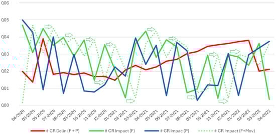
Figure 3.
Impact on economic activities by external factor COVID-19. This figure presents normalized credit risk impact values across economic activity types under different pandemic-related external factor scenarios. The vertical axis represents a normalized metric (ranging from 0 to 1) that quantifies the relative intensity of impact observed for each external factor. External factor notations: F = COVID-19 Deaths, P = COVID-19 Positive Cases, F + P = Combined Impact of COVID-19 Deaths and Positive Cases, F + Mov = Combined Impact including Mobility Restrictions.
Figure 4 illustrates the impact of social unrest and climatic factors on economic activity from December 2022 to September 2023. It compares delinquency rates with the economic impact of social unrest, weather, and temperature anomalies, and shows significant spikes during periods of intensified external disruptions.
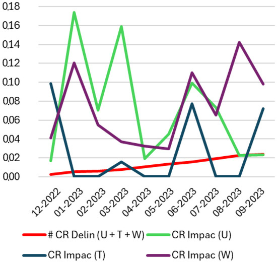
Figure 4.
Impact on economic activities by external factors: social unrest and climatic events. This figure presents normalized credit risk impact values across economic activity types under different external factor scenarios. The vertical axis represents a normalized impact metric (ranging from 0 to 1) that reflects the relative intensity of the effect across sectors. External factor notations: U = social unrest, T = temperature anomaly, W = weather-induced road blockages, U + T + W = combined effect of social unrest, temperature anomaly, and road blockages.
3.2.3. Research Strategy
The evaluation period for this study is defined based on the behavior of the monthly classification variables, starting from the onset of the impact of EF until stabilization as shown in Figure 3 and Figure 4. Stabilization is defined as the point at which the slope of the curve representing the proportion of bad payers (red line) began to level off.
Evaluation Periods
- COVID-19: The evaluation period spans March 2020 to January 2022. Loans disbursed until October 2021 are included to account for a 60-day grace period before delinquencies appeared, ensuring unbiased results (Figure 3).During the analysis of the COVID-19 external factors, it was identified that the trends in the number of positive cases and deaths often showed opposing behaviors. To address this, an additional experiment was conducted, in which the death curve was shifted from one period to the right, referred to as the COVID MOV. This adjustment considered the estimated incubation period of the disease and the time to potential fatality, typically ranging from 2 to 3 weeks. By aligning the death data with this temporal delay, this analysis aimed to capture the causal relationship between disease progression and its impact on credit delinquency rates. This methodological adjustment is illustrated in Figure 3 (green dotted line).
- Social Unrest and Climate Factors: Data from December 2022 to September 2023 were analyzed, with loans disbursed up to June 2023 considered under the same grace period logic (Figure 4).
In addition, the dataset includes a variable that identifies whether a credit was backed by a government guarantee. Based on this variable, two experimental configurations were defined: one including all government-backed credits (WGB_CR), and another excluding them (WOGB_CR), to evaluate potential biases introduced by public credit support programs.
To assess the influence of external stressors on credit risk, multiple experimental scenarios were constructed using different combinations of observed external factors (see Table 6). These include a baseline scenario SFE, as well as scenarios incorporating COVID-19-related metrics such as fatalities (F), confirmed positive cases (P), and a combined F + P scenario. Additionally, a variation labeled COVID MOV was considered, shifting fatality data forward by one month to account for incubation and reporting delays.
Table 6.
Acronyms of evaluated scenarios.
Other scenarios focused on sociopolitical and environmental disruptions, including social unrest indicators (U), temperature anomalies (T), and road blockages caused by extreme weather (W). Combined scenarios such as T + W (climatic anomalies and road disruptions) and U + T + W (integrating social unrest, climate variability, and climate-induced blockages) were also included to evaluate compound effects.
Data Preprocessing
- Data normalization and standardization were applied to homogenize the scales [53].
- Features with correlations above 90% were removed to prevent redundancy.
- SMOTE was used to balance the dataset [54].
Machine Learning Models
We implemented the following models to evaluate the binary classification tasks, prioritizing interpretability and predictive performance:
- Traditional Models: Linear Discriminant Analysis (LDA), Quadratic Discriminant Analysis (QDA), and k-Nearest Neighbors (KNN) [54].
- Advanced Models: Perceptron (PERCEP), Multi-layer Perceptron (MLP), Random Forest (RF) [3], Ridge Regression (Ridge) [55], and Extreme Gradient Boosting (XGB) [56].
- Explainable Models:
- –
- Explainable Neural Network (XNN), which directly integrates interpretability into the model architecture [17].
- –
- Explainable Boosting Machines (EBM), a method that combines high accuracy with feature interpretability through additive modeling [57].
- Feedforward Neural Networks: Variants of Feedforward Neural Networks (FFNN) were explored:
- –
- Standard Feedforward Neural Network (FFN): A classical architecture used as a baseline for comparison.
- –
- Feedforward Neural Network with Sparse Regularization (FFNSP): Incorporates sparsity constraints to enhance generalization and reduce overfitting.
- –
- Feedforward Neural Network with Local Penalty Regularization (FFNLP): Local penalty terms are applied to balance feature contributions and improve interpretability.
- Deep Learning: Convolutional Neural Networks (CNN) were included for their ability to capture complex relationships in both spatial and temporal data [25]. Although CNN are traditionally applied to image or time-series data, in this study, each tabular instance was reshaped into a 2D tensor of shape , allowing the use of 1D convolutional layers to capture localized patterns across the feature vector. This approach has been successfully applied in previous studies involving structured tabular data [58].
Each model was trained and evaluated using a stratified 10-fold cross-validation protocol, ensuring balanced class representation across folds [26]. In each fold, 90% of the data was used for model development and 10% was held out for testing. Within the development portion, 75% was used for training and 25% for internal validation, enabling unbiased hyperparameter tuning. We employed a combination of grid search and Bayesian optimization to identify optimal model configurations.
All performance metrics—including ACC, AUC, F1, and KS—were computed separately on the validation and test partitions for each fold. The final results reported in the manuscript correspond to the average values obtained across the 10 test folds.
Explainability with XAI
To address concerns about interpretability, SHAP and LIME were applied to identify the most influential features in predicting credit delinquency both before and after incorporating EF. Models such as XNN and EBM provided native interpretability, complementing these post hoc methods.
Statistical Evaluation
The impact of EF on model performance was assessed using Student’s t-test (Equation (3)), applied to metrics such as ACC, AUC, KS and F1 from the cross-validation folds, with a significance level of :
The terms represent the following:
- : mean of metrics from ten folds;
- : hypothetical mean under the null scenario;
- s: standard deviation of metrics;
- n: number of folds ().
Economic Activity Relevance
The dataset, comprising 367,000 loans (see Table 2), was analyzed based on its concentration across economic activities. This analysis is particularly relevant, as the impact of EF on these activities amplifies exposure to credit risk. The distribution of loans is as follows:
- 80% Concentration: 80% of the loans are concentrated in 78 economic activities.
- 99% Concentration: 99% of the loans are concentrated in 326 economic activities.
- 100% Concentration: 100% of the loans are distributed across 660 economic activities.
Figure 5 illustrates these groupings, highlighting the increased dispersion and noise as the number of activities increases. To ensure a comprehensive analysis, the results were further examined by including and excluding loans affected by government-backed programs, thereby isolating the potential biases introduced by such interventions.
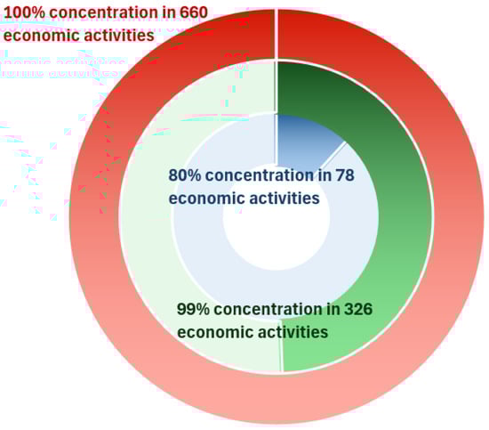
Figure 5.
Relevance of Economic Activity.
Research Limitations and Biases
While this study provides valuable insights into the influence of EF on credit delinquency predictions, several limitations and potential biases must be considered:
- Context-Specific Findings: The analysis is based on data from the Peruvian context, which may limit the generalizability to other regions with different economic, social, and environmental dynamics. Future research should incorporate external validation by using datasets from diverse geographical areas to evaluate the transferability of the proposed methodology.
- Training Data Bias: Dataset imbalances and the under-reporting of delinquency during government interventions may introduce biases. Although SMOTE has been used to address class imbalances, residual biases related to data collection practices or policy impacts may persist.
- Model Transparency: While explainability techniques such as SHAP, LIME, and interpretable models (e.g., XNN and EBM) have been employed, the use of black-box models like CNN and XGB remains a challenge. This lack of inherent transparency could hinder their applicability to financial institutions, where explainability is crucial for regulatory compliance and stakeholder trust.
- Temporal Assumptions: The assumption that loans disbursed near the evaluation cutoff reflect the grace period impacts may not fully account for the delayed delinquency effects, particularly for loans with extended repayment terms.
- Data Quality and Noise: External factor measurements and institutional datasets may contain noise or inaccuracies that could affect model performance, despite preprocessing steps such as normalization and standardization. Future work should explore advanced noise-reduction techniques.
- Researcher Influence: Prior domain knowledge and experience can introduce subtle biases in model selection, EF, or preprocessing decisions. To mitigate this, the study adhered to best practices such as k-fold cross-validation, rigorous statistical testing, and methodological transparency.
Despite these limitations, the methodological rigor applied in this study, including robust preprocessing, comprehensive statistical validation, and the integration of explainable models, provides a solid foundation for future research. The findings highlight the need for the further exploration of EF impacts in broader contexts, paving the way for more robust, interpretable, and generalizable credit risk assessment frameworks.
4. Results
4.1. Stationarity Analysis and Dataset Integration
In this analysis, “economic activities” refer to the internal sector classification codes provided by the financial institution FMOD. These codes represent a customized segmentation structure used to group clients based on their type of business or productive sector, and are derived from operational risk models. Although not fully equivalent to official international standards, these codes are conceptually aligned with the International Standard Industrial Classification of All Economic Activities (ISIC Rev. 4), maintained by the United Nations Statistics Division. (https://unstats.un.org/unsd/classifications/Econ/isic, accessed on 5 April 2025).
Specifically, the evaluation window from April 2018 to February 2020 (as shown in Table 7) contains 718 unique activity codes, each linked to credit operations that remained active during that period. Other periods in the table include subsets of these activities, depending on whether data on overdue loans were available within each respective evaluation window.
Table 7.
Economic activity delinquency stationarity.
To assess the influence of EF on economic activity delinquency, we first applied the Dickey–Fuller stationarity test (see Equation (1)) to the normalized daily time series covering the period from January 2016 to September 2023 (see Table 2). These time series represent the number of delinquency days associated with the economic activities under study, examined both in periods with EF and without EF [47].
Key Stationarity Findings
Table 7 shows that, in periods without EF, between 90% and 91% of the activities exhibit non-stationary delinquency patterns, while 6–7% exhibit stationarity, and around 3% are indeterminate. In contrast, periods with EF present a lower proportion of non-stationary activities (75–85%) and a higher proportion of stationary (6–22%) or indeterminate patterns (2–9%). These differences suggest that exogenous shocks, such as pandemics, social unrest, or climatic disruptions, can induce more persistent or complex delinquency behaviors, consistent with similar observations in other emerging economies.
To assess the influence of EF on economic activity delinquency, the Dickey–Fuller stationarity test was applied (see Equation (1)) to the normalized time series of daily frequency. These series represent the days of delinquency associated with the analyzed economic activities. The data used for this analysis cover the period from January 2016 to September 2023 (see Table 2). The analysis was performed for both periods influenced by EF and those without EF [47].
The results indicate that during periods without EF influence, between 90% and 91% of economic activities exhibited non-stationary delinquency, while 7% and 6% showed stationarity. Additionally, 3% of the activities fell into the “indeterminate” category, where stationarity could not be conclusively determined. In periods with EF influence, the proportion of non-stationary activities decreased to 75% and 85%, whereas stationary activities increased to 22% and 6%. The “indeterminate” category also showed slight variations, with 2% and 9% of the activities falling into this group.
The “indeterminate” classification, though a minority, highlights cases where delinquency patterns are less predictable or fall outside the thresholds for stationarity detection. This suggests that EF may not only influence stationarity directly but may also introduce complexity in delinquency patterns, making it harder to classify definitively.
This behavior may be explained by the risk management practices of financial institutions during stable periods. In the absence of external shocks, institutions are more capable of identifying early signs of payment delays and can adjust their credit exposure accordingly—often by suspending or restricting lending to high-risk segments. These interventions disrupt emerging trends, resulting in more irregular default behavior that tends to deviate from stationary assumptions due to abrupt shifts in mean or variance.
Conversely, during systemic external shocks—such as pandemics or climate disruptions—multiple economic sectors experience distress concurrently, reducing the institution’s ability to react. This leads to prolonged and homogeneous delinquency patterns across broader borrower groups, increasing the likelihood of stationarity in the associated time series.
These findings are summarized in Table 7, which provides a detailed breakdown of the stationarity classifications across the different periods of evaluation. The results underscore the dynamic impact of external factors on the stationarity of delinquency days in economic activities, reinforcing the need to account for these factors in economic analyses and credit risk prediction models.
4.2. Definition of Evaluated Scenarios and Causality Testing
To evaluate the seasonal impact of EF on the default behavior of economic activities, the Granger causality test (see Equation (2)) was applied to the time series representing the days of default for each economic activity, in conjunction with the time series of each EF. For simplicity, a binary value of 1 was assigned when the p-value was less than 0.05, indicating statistically significant causality, and 0 otherwise. This binary classification was performed every month to effectively capture temporal variations.
The results of this causality analysis were subsequently integrated into the credit dataset and associated with the corresponding economic activity and period under analysis. Additionally, a global binary classification variable was calculated and appended to the dataset to identify the payment quality of credit holders (good or bad payers) based on monthly delinquency data. This enriched dataset provided the foundation for applying Algorithm 1 to the established datasets (see Figure 5) to compute the ACC, AUC, KS, and F1 metrics for the evaluated machine learning models. These models were assessed across the scenarios listed in Table 6. Based on the values obtained, the differences between the scenarios that include EF and SFE scenarios were calculated as shown in Table 8.
| Algorithm 1 Dataset evaluation using ML algorithms. |
|
Table 8.
Acronyms of the results for the evaluated scenarios.
The performance metrics (ACC, AUC, KS and F1) derived from the application of machine learning models for the binary classification of good and bad payers, evaluated across datasets stratified by relevance to established scenarios, are presented in Table A1, Table A2, Table A3, Table A4, Table A5, Table A6, Table A7, Table A8, Table A9, Table A10, Table A11, Table A12, Table A13, Table A14, Table A15 and Table A16 in Appendix A. These tables provide a detailed comparative analysis of the scenarios with and without the inclusion of EF related to COVID-19, social unrest, and climate change.
Additionally, Table A17, Table A18, Table A19, Table A20, Table A21 and Table A22 in Appendix A identify the machine learning models that achieved statistically significant improvements in their classification metrics when the EFs were incorporated. These tables delineate the conditions under which specific models demonstrate enhanced predictive capabilities, providing critical insights into the sensitivity and adaptability of various machine learning approaches to external factors.
The comprehensive dataset from these experiments forms a robust foundation for addressing the research questions that underpin this study. Given the extensive volume of information presented, the subsequent discussion focuses on the most significant results, with direct references to the relevant tables to highlight critical findings and their implications for predictive modeling under diverse scenarios.
- RQ1. How did the COVID-19 pandemic, through factors such as positive cases and mortality rates, influence credit defaults in different economic activities?
The first research question is focused on understanding the impact of the COVID-19 pandemic on credit delinquency, particularly through the inclusion of variables such as confirmed infections and mortality. A comparative analysis was conducted between baseline scenarios SFE and those influenced by pandemic conditions, including a time-shifted mortality scenario (COVID MOV). Across all evaluation metrics—AUC, ACC, KS, and F1—the results consistently indicate a marked shift in credit risk behavior during pandemic periods.
Among the pandemic-related variables, mortality rates—especially when temporally aligned to reflect delayed economic effects—proved to be the most influential predictor of default. This effect was most evident in the 3. D80 dataset, which encompasses high-contact economic sectors that are particularly vulnerable to pandemic restrictions and health crises. In this scenario, the inclusion of lag-adjusted mortality data significantly enhanced model performance, suggesting that delayed health outcomes capture the real-world propagation of credit risk better than contemporaneous case counts alone.
The presence of government-backed credit mechanisms also played a decisive role. In datasets where such guarantees were included (WGB_CR), the predictive impact of the pandemic was partially cushioned, resulting in lower volatility and more stable classification outcomes. Conversely, in non-guaranteed portfolios (WOGB_CR), default risks increased substantially, reflecting the lack of institutional buffers.
In terms of model performance, CNN and XGB emerged as the most effective across all partitions, consistently achieving top-tier predictive accuracy and discrimination. While models such as EBM demonstrated improvements in specific scenarios—particularly under external stressors—others like XNN exhibited limited effectiveness, especially in pandemic-related contexts, which constrained their applicability despite their inherent interpretability features.
These findings are further reinforced by the interpretability analyses shown in Figure 6, where SHAP and LIME techniques reveal how the relative importance of predictive features shifts across scenarios. Variables related to debt burden and origination characteristics gained or lost prominence depending on whether pandemic indicators were present, reflecting the models’ dynamic response to exogenous health shocks.
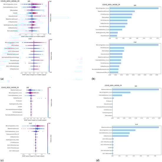
Figure 6.
Top 10 features between without external factors (SFE) and COVID-19 stress scenarios (F + P). (a) XGB SHAP analysis, (b) XGB LIME analysis, (c) CNN SHAP analysis, and (d) CNN LIME analysis. Legend: F = COVID-19 confirmed cases; P = COVID-19 deceased; F + P = Combined scenaries; Mov = Mobility restrictions; WGB_CR = With Government-Backed Credit; WOGB_CR = Without Government-Backed Credit.
In summary, the COVID-19 pandemic had a substantial and measurable effect on credit delinquency patterns. Mortality—particularly when time-shifted—proved to be the most impactful factor, and its inclusion substantially improved model robustness. Government interventions, while partially effective, could not fully suppress the delinquency risks in the most exposed segments. These insights underscore the value of integrating lag-sensitive external variables into credit risk modeling, especially for sectors with heightened structural vulnerability.
Figure 6 provides interpretability insights into the predictive behavior of the XGB and CNN models under both baseline (SFE) and COVID-affected (F + P) scenarios, using SHAP and LIME explainability techniques.
Figure 6a,b illustrate the SHAP and LIME results for the XGB model, respectively. Under the SFE scenario, features such as MicroOrigination_Score, Overindebtedness_ Score, and MaxInternalAmount exhibit the greatest impact on prediction outputs. In the F + P setting, variables directly linked to pandemic conditions—such as 2021-04Positive Cases and 2020-10Deceased—emerge alongside financial indicators, suggesting an integration of external health shocks into the model’s risk prioritization.
Figure 6c,d display the corresponding SHAP and LIME analyses for the CNN model. Similar to XGB, the CNN model assigns greater relevance to features such as MaxInternalAmount and MicroOrigination_Score under the baseline (SFE) scenario. In the F + P scenario, feature importance shifts toward pandemic-related variables and demographic indicators (e.g., 2020-09PositiveCases, 2020-09Deceased, DAResDirection, Gender), reflecting the model’s responsiveness to contextual changes introduced by COVID-19.
Together, these visualizations underscore the dynamic interaction between model architecture and scenario context, revealing how external stressors—particularly COVID-19—reshape the prioritization of financial and behavioral risk indicators within advanced machine learning models.
- RQ2. To what extent do climate change indicators, such as temperature anomalies and road blockages due to weather, impact credit delinquency patterns?
The analysis of climate-related external factors—specifically temperature anomalies (T) and weather-induced road blockages (W)—reveals a measurable and statistically significant influence on credit delinquency behavior. While the magnitude of this effect is generally more moderate compared to pandemic-related variables, it remains consistent across scenarios and data partitions.
Table A9, Table A10, Table A11 and Table A12 (WGB_CR) and Table A13, Table A14, Table A15 and Table A16 (WOGB_CR) show notable improvements in classification metrics such as ACC, AUC, KS, and F1 upon including climate variables. These gains are particularly prominent in the absence of government guarantees, where borrowers are more directly affected by logistical disruptions. In portfolios without policy support (WOGB_CR), the effect of weather-related blockages is accentuated, often contributing to delays in income flows and operational closures—factors that increase credit risk exposure.
From a comparative perspective, the predictive gains attributed to climate anomalies may not be as large as those observed under pandemic mortality scenarios, yet they are highly context dependent. For instance, improvements in AUC of up to 3% and accuracy gains of over 30% have been recorded in neural network models, especially when the economic activities under analysis are concentrated in geographically exposed sectors. This supports the findings of [30], who demonstrated that road infrastructure disruptions can propagate liquidity shocks and elevate default risk, particularly in informal or underserved lending markets.
Figure 7 illustrates how the XGB model integrates climate variables into its decision structure, ranking them alongside key behavioral and demographic attributes. This interpretability result reaffirms that exogenous environmental stressors, while external to borrower control, are internalized by advanced algorithms as significant contributors to credit delinquency prediction.
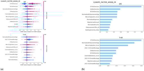
Figure 7.
Top 10 features between scenarios without external factors (SFE) and with climate external factors (T + W): (a) XGB SHAP analysis. (b) XGB LIME analysis. Legend: SFE = Scenario without external factors; T = Temperature Anomaly; W = Climate Blockage; T + W = Combined scenarios; WGB_CR = With Government-Backed Credit; WOGB_CR = Without Government-Backed Credit.
In sum, the inclusion of climate indicators in credit risk models enhances their ability to reflect real-world disruptions and borrower vulnerability. The observed performance improvements are not only statistically valid but also economically meaningful, underscoring the importance of incorporating climate-related risks into financial predictive systems, particularly in emerging markets subject to environmental volatility.
Figure 7 provides interpretability insights into the behavior of the XGB model under climate-related stress conditions. Figure 7a presents the SHAP analysis comparing the baseline scenario SFE and the scenario that includes both temperature anomalies and weather-induced road blockages (T + W). The visualization highlights the ten most influential features in each setting, with color gradients indicating the direction and intensity of their contribution to the model’s predictions. High feature values are represented in red and low values in blue, allow a clear interpretation of how variable magnitudes relate to increased or decreased credit risk.
Figure 7b displays the corresponding LIME analysis for the same dataset (CLIMATE_ FACTOR_WOGB_CR). In both scenarios, DTResDirection emerges as the most critical driver of classification outcomes. Notably, under the T + W scenario, Gender gains relevance, suggesting that climate-related externalities may interact differently with sociodemographic characteristics. This contrast between the SFE and T + W contexts reinforces the need to account for latent vulnerabilities when modeling credit risk under environmental stress.
Together, these interpretability results confirm that the inclusion of climate factors not only enhances model accuracy but also reconfigures the internal prioritization of risk features. This dynamic adaptation reflects the capacity of machine learning models like XGB to absorb and reflect external shocks through learned decision boundaries.
- RQ3. What is the relationship between credit delinquency and social unrest, considering disruptions to economic activities and societal stability?
Social unrest—manifested through protests, strikes, and other large-scale disruptions—can severely affect economic activity by limiting mobility, reducing consumer demand, and disrupting informal and formal markets. These effects become particularly salient in borrower segments highly dependent on local or face-to-face interactions.
Our analysis confirms that the inclusion of social unrest indicators (U) in the datasets yields statistically significant improvements in credit delinquency prediction. These improvements are evident in both WGB_CR and WOGB_CR portfolios, although the magnitude of the effect is more pronounced in the latter. This distinction highlights the protective role of policy guarantees, which tend to buffer the financial impact of systemic disruptions.
In terms of model responsiveness, CNN, and XGB exhibit the highest sensitivity to unrest scenarios, achieving notable gains in metrics such as AUC, ACC, KS, and F1. Classical models, including LDA and Ridge, also show moderate but statistically consistent improvements. Notably, in the 3. D80 dataset—focused on high-contact economic activities—the accuracy and discrimination capacity of models improve substantially under social unrest scenarios, suggesting that these sectors are disproportionately vulnerable to institutional instability.
Interpretability analyses provide further insight. As shown in Figure 8, SHAP values for CNN and XGB highlight a shift in feature relevance when social unrest variables are introduced. Features such as Overindebtedness_Score and MaxInternalAmount become more prominent, reflecting the increased importance of financial stress indicators in volatile sociopolitical contexts.
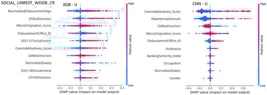
Figure 8.
SHAP XGB and CNN: Top 10 Features in scenarios with social unrest (U). Legend: U = social unrest, represented by events of civil protest and political instability registered in 2023; WGB_CR = with government-backed credit; WOGB_CR = without government-backed credit.
In summary, the presence of social unrest introduces measurable and context-sensitive volatility in credit delinquency behavior. Its integration into predictive models not only improves classification performance but also enhances the capacity to identify borrower segments at heightened risk. These findings support the existing literature on the financial impacts of sociopolitical instability and underscore the importance of incorporating such variables into credit risk assessments, particularly in emerging economies where unrest events are recurrent and unevenly absorbed by the population.
Figure 8 presents the SHAP feature importance analysis for the XGB and CNN models under the “U scenarios” in the SOCIAL_UNREST_WOGB_CR dataset. The top 10 influential features are shown for each model, with Overindebtedness_Score and MaxInternalAmount being particularly significant in both, highlighting their impact on the model predictions.
- RQ4. How do the combined effects of external factors (COVID-19, climate change, and social unrest) contribute to variations in credit delinquency, and what are the most influential factors?
The combination of external factors—pandemic severity, climatic anomalies, and sociopolitical instability—amplifies the complexity and unpredictability of credit behavior. When analyzed jointly, these variables generate compounded stress conditions that exert a stronger influence on delinquency patterns than any of them in isolation. This effect is particularly evident in the absence of government-backed guarantees (WOGB_CR), where borrowers are fully exposed to systemic shocks.
Empirical results from multifactor scenarios, such as U + T + W and Climate+Unrest, show a higher density of statistically significant gains across all evaluation metrics. Notably, mortality indicators (especially in lag-adjusted form, i.e., COVID MOV) remain the dominant predictor of default, reflecting the profound economic dislocation associated with fatal health outcomes. Climatic variables, although more moderate in their individual contribution, reinforce vulnerability in certain borrower segments, particularly when the infrastructure is disrupted by weather-related events. Social unrest introduces further pressure by destabilizing labor income and limiting business continuity.
Model behavior under combined factor scenarios reveals distinct patterns. XGB consistently ranks as the most resilient and adaptive model, achieving significance across all multifactor experiments. CNN also demonstrates strong performance, although with some sensitivity to the structure of the input data and the intensity of external stressors. While XNN was included as an interpretable neural model, its performance was inconsistent, limiting its contribution beyond methodological comparison. Classical models such as Ridge and LDA continue to offer baseline robustness, particularly in datasets with partial shielding (e.g., WGB_CR), although their gains remain smaller and more scenario dependent.
Figure 9 supports these findings by showing the SHAP analyses for CNN, XGB, and XNN in scenarios combining all external factors. Variables such as MaxInternalAmount, Overindebtedness_Score, and DAResDirection consistently emerge as top predictors, reflecting how borrower financial behavior interacts with macro-level disruptions. The shifting prominence of these features across models underscores the necessity of interpretability tools to contextualize model predictions in complex environments.
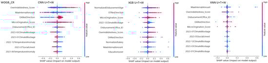
Figure 9.
SHAP CNN, XGB, and XNN: Top 10 features in scenarios combining external factors. Legend: U = social unrest (e.g., protests and road blockages); T = temperature anomalies; W = climate blockages; U + T + W = combined scenario including all three external factors; WOGB_CR = credit risk portfolio excluding government-backed loans.
In conclusion, the combined influence of external shocks intensifies credit risk dynamics and reveals structural fragilities in both the borrower base and the credit portfolios. The models’ ability to detect and adapt to these stressors is contingent not only on the algorithmic design but also on how exogenous variables are incorporated, preprocessed, and aligned temporally. These findings reinforce the importance of building integrated, context-aware credit risk models—particularly in economies where multiple external threats converge and the margin for institutional response is limited.
5. Discussion and Research Implications
This study examined how credit delinquency prediction is affected by the incorporation of EF, including pandemic severity, climate anomalies, and social unrest. The findings demonstrate that these variables introduce significant and context-dependent shifts in credit behavior, particularly in scenarios without government-backed guarantees. At the same time, the process revealed methodological challenges that are increasingly relevant in the application of ML in dynamic financial environments.
The first challenge relates to the quality and availability of data on external disruptions. Publicly available records on COVID-19 mortality, weather events, and protest activity often lack consistency and timeliness, complicating their integration into high-frequency credit datasets. Similar issues have been noted in prior empirical efforts conducted in Peru, where the construction of reliable time series for economic modeling has required substantial preprocessing [28,29]. In this study, the alignment of mortality data through temporal shifts proved essential, as it revealed the delayed but pronounced influence of pandemic fatalities on repayment capacity.
Another source of complexity was the divergence between credit portfolios with and without public guarantees. Government-backed loans mitigated part of the risk during systemic shocks but also altered the underlying statistical distribution of defaults. This distinction made model generalization more challenging but also more necessary for understanding the buffering effects of financial policy. Prior studies in Latin America suggest that the performance of ML classifiers can vary significantly depending on whether policy instruments like emergency credit programs are present [27].
Overfitting risks were also non-trivial, particularly when combining multiple exogenous factors in deep learning architectures. Although regularization and cross-validation strategies were implemented, the complexity of models such as CNN and XNN occasionally reduced transparency. While post hoc interpretability tools like SHAP and LIME help uncover shifts in feature relevance across scenarios, they do not entirely resolve concerns regarding model opacity—especially in contexts where regulatory clarity and explainability are essential [30,59].
Despite these challenges, several insights emerge. Mortality-related variables—especially when time-lagged—exert the strongest influence on credit behavior, particularly in high-contact economic sectors. Climate-related disruptions, though more moderate in effect, consistently improved predictive accuracy, especially in vulnerable portfolios. Social unrest also introduces nonlinear shocks, further reinforcing the need for adaptive models that account for real-world volatility.
The integration of multiple external stressors revealed a compounding effect on delinquency, a finding that conventional econometric approaches may fail to capture. Tree-based and neural models, particularly XGB and CNN, showed the greatest adaptability in this regard. At the same time, classical models like Ridge maintained stable performance under certain constrained scenarios, suggesting a role for hybrid modeling strategies.
In the Peruvian context, these findings align with recent efforts to modernize credit risk assessment through advanced analytics. Several local studies highlight the value of incorporating contextual variables and borrower segmentation into scoring systems, particularly in the wake of the pandemic and its economic aftermath [29,35]. Internationally, there is growing consensus around the importance of multidimensional modeling frameworks that include environmental and social dimensions alongside traditional financial indicators.
Overall, this study contributes to the ongoing development of risk prediction systems capable of responding to complex and evolving realities. It underscores the importance of aligning exogenous variables not only temporally but also conceptually with the credit cycle. Future implementations of ML in finance—particularly in emerging economies—should prioritize data interoperability, scenario partitioning, and explainable design to ensure both accuracy and transparency in risk-based decision-making.
6. Conclusions and Future Research
This study has demonstrated that credit delinquency prediction improves significantly when EF—such as COVID-19 severity, climate anomalies, and social unrest—are systematically integrated into machine learning workflows. Using a multi-scenario design and high-resolution time series, the models captured both the direct and delayed effects of these external shocks across various economic activities and portfolio compositions.
By incorporating explanatory tools such as SHAP and LIME, and validating the results with formal stationarity and causality tests, the study provided both predictive and interpretive value. Notably, the performance of key metrics—AUC, ACC, KS, and F1—was significantly enhanced in models exposed to time-shifted mortality and climate-related variables. This confirmed that delayed systemic shocks (e.g., COVID-related deaths) exert stronger predictive influence than contemporaneous infection rates, and that road infrastructure disruptions propagate liquidity risks, particularly in non-guaranteed portfolios.
The comparative evaluation revealed that CNN and XGB consistently outperformed other models across multiple relevance partitions and scenarios. While EBM proved especially useful in contexts requiring greater model transparency, XNN served as an exploratory reference for intrinsically interpretable architectures, although its predictive effectiveness was limited in high-volatility scenarios. Moreover, the role of government-backed guarantees emerged as central: their presence moderated the effects of external crises, whereas their absence magnified the volatility and default risks observed in the models.
Overall, these findings offer a scenario-driven framework for understanding how systemic shocks affect credit behavior. This framework is replicable and adaptable to emerging economies facing concurrent crises, combining domain-sensitive data transformations (e.g., lag structures) with advanced modeling and interpretability techniques. Importantly, the integration of KS and F1 metrics deepens the evaluation of not just model accuracy but also the discriminatory power and balance between false positives and false negatives—factors critical to financial risk management and regulatory compliance.
Looking forward, several research directions are both relevant and necessary. First, the use of static lag structures could be extended through adaptive or dynamic lag modeling, particularly in the case of gradual-onset crises such as climate change or prolonged social instability. Second, cross-regional replication would test the generalizability of these findings in other vulnerable markets, where the interaction between policy buffers and external shocks may differ. Third, in-depth analysis of credit policies—such as emergency moratoria or targeted guarantees—would enable the finer-grained modeling of institutional effectiveness under stress. Finally, explainability remains a methodological frontier: while SHAP and LIME provide insights, future work could explore intrinsically interpretable models or causal frameworks that support regulatory transparency and stakeholder trust.
In conclusion, this research confirms the value of integrating multidimensional exogenous variables into credit risk modeling, offering a robust and explainable approach to capturing volatility in increasingly complex economic environments. As global financial systems face overlapping crises, such tools will become indispensable for promoting resilience, fairness, and informed decision-making in credit allocation.
Author Contributions
Conceptualization, J.N. and J.H.; methodology, J.N.; validation, J.N., L.R. and J.H.; formal analysis, J.N., J.C. and J.H.; investigation, J.N.; resources, J.N.; writing—original draft preparation, J.N.; writing—review and editing, J.N., L.R., J.C. and J.H.; visualization, J.N. and J.C.; supervision, J.H.; project administration, J.N. All authors have read and agreed to the published version of the manuscript.
Funding
This research received no external funding.
Institutional Review Board Statement
Not applicable.
Informed Consent Statement
Not applicable.
Data Availability Statement
The datasets presented in this study are partly publicly available and partly proprietary. Public datasets (COVID-19 cases, deaths, road blockages, and temperature anomalies) are accessible through the official URLs listed in Table 2. Proprietary financial datasets (credit delinquency activity and credits with external factors) were used under confidentiality agreements and have been anonymized and aggregated. Metadata, modeling programs, and experimental results have been deposited and are openly available at Zenodo: https://zenodo.org/records/14890903. Further inquiries can be directed to the corresponding author(s).
Conflicts of Interest
The authors declare no conflicts of interest.
Appendix A. Results Tables
Table A1.
Average AUC and ACC across 10 folds of ML models with COVID EF WGB_CR, by evaluated scenario and relevance groups.
Table A1.
Average AUC and ACC across 10 folds of ML models with COVID EF WGB_CR, by evaluated scenario and relevance groups.
| AUC (%) | ACC (%) | |||||||||||||
|---|---|---|---|---|---|---|---|---|---|---|---|---|---|---|
| Scenarios | Results | Scenarios | Results | |||||||||||
| SFE | P | F + P | F | P - SFE | F + P - SFE | F - SFE | SFE | P | F + P | F | P - SFE | F + P - SFE | F - SFE | |
| WGB_CR | ||||||||||||||
| 1. D100 | ||||||||||||||
| cnn | 72.82 | 73.63 | 74.09 | 74.09 | 0.82 | 1.28 | 1.27 | 67.49 | 70.07 | 70.18 | 70.14 | 2.58 | 2.69 | 2.65 |
| ebm | 81.13 | 81.23 | 81.42 | 81.26 | 0.10 | 0.29 | 0.13 | 74.84 | 74.94 | 75.05 | 74.93 | 0.09 | 0.20 | 0.08 |
| ffn | 72.30 | 72.56 | 72.39 | 73.38 | 0.26 | 0.10 | 1.08 | 66.74 | 65.24 | 66.15 | 66.14 | −1.50 | −0.59 | −0.60 |
| ffnlp | 72.11 | 72.35 | 72.41 | 72.72 | 0.25 | 0.30 | 0.61 | 66.28 | 67.55 | 65.64 | 65.19 | 1.27 | −0.64 | −1.09 |
| ffnsp | 72.31 | 72.31 | 71.42 | 72.77 | 0.00 | −0.89 | 0.47 | 66.40 | 66.45 | 64.67 | 65.59 | 0.05 | −1.73 | −0.81 |
| knn | 67.21 | 66.92 | 66.93 | 66.93 | −0.29 | −0.28 | −0.28 | 63.23 | 63.00 | 62.97 | 62.98 | −0.22 | −0.26 | −0.24 |
| lda | 67.23 | 68.01 | 68.54 | 68.25 | 0.78 | 1.31 | 1.02 | 63.09 | 63.74 | 64.09 | 63.77 | 0.65 | 1.00 | 0.67 |
| mlp | 69.30 | 70.83 | 71.17 | 70.47 | 1.53 | 1.87 | 1.17 | 60.82 | 63.26 | 63.58 | 62.87 | 2.44 | 2.76 | 2.06 |
| percep | 57.96 | 58.44 | 59.88 | 59.46 | 0.48 | 1.92 | 1.50 | 44.58 | 57.99 | 56.37 | 49.31 | 13.41 | 11.78 | 4.73 |
| qda | 67.44 | 66.98 | 65.81 | 67.17 | −0.46 | −1.63 | −0.27 | 52.50 | 54.01 | 54.13 | 53.72 | 1.52 | 1.64 | 1.22 |
| rf | 81.74 | 81.51 | 81.21 | 81.46 | −0.23 | −0.53 | −0.29 | 75.51 | 75.44 | 75.22 | 75.48 | −0.07 | −0.29 | −0.03 |
| ridge | 66.94 | 67.55 | 68.05 | 67.81 | 0.62 | 1.12 | 0.87 | 62.93 | 63.39 | 63.70 | 63.43 | 0.46 | 0.77 | 0.50 |
| xgb | 80.76 | 81.00 | 81.10 | 81.07 | 0.23 | 0.33 | 0.30 | 74.77 | 74.98 | 75.03 | 74.98 | 0.21 | 0.26 | 0.22 |
| xnn | 50.14 | 50.38 | 50.10 | 50.37 | 0.24 | −0.05 | 0.22 | 53.42 | 57.99 | 62.76 | 54.22 | 4.57 | 9.34 | 0.80 |
| 2. D99 | ||||||||||||||
| cnn | 72.75 | 73.60 | 74.27 | 73.57 | 0.86 | 1.52 | 0.83 | 67.04 | 70.03 | 70.42 | 69.97 | 2.98 | 3.37 | 2.93 |
| ebm | 81.04 | 81.24 | 81.37 | 81.24 | 0.19 | 0.33 | 0.20 | 74.77 | 74.93 | 75.04 | 74.94 | 0.16 | 0.28 | 0.18 |
| ffn | 72.69 | 72.38 | 71.50 | 71.55 | −0.31 | −1.20 | −1.14 | 66.07 | 65.94 | 65.86 | 65.75 | −0.14 | −0.21 | −0.32 |
| ffnlp | 71.71 | 72.81 | 72.16 | 72.45 | 1.09 | 0.44 | 0.74 | 65.27 | 66.83 | 66.28 | 65.94 | 1.56 | 1.02 | 0.67 |
| ffnsp | 72.58 | 73.11 | 72.58 | 72.99 | 0.53 | −0.00 | 0.41 | 63.93 | 65.34 | 66.81 | 66.17 | 1.41 | 2.87 | 2.24 |
| knn | 67.10 | 66.88 | 66.88 | 66.88 | −0.22 | −0.21 | −0.21 | 63.24 | 63.02 | 63.02 | 63.04 | −0.23 | −0.22 | −0.21 |
| lda | 67.17 | 67.92 | 68.46 | 68.19 | 0.75 | 1.29 | 1.02 | 63.07 | 63.68 | 64.04 | 63.78 | 0.60 | 0.96 | 0.70 |
| mlp | 69.79 | 68.93 | 69.62 | 68.70 | −0.86 | −0.16 | −1.08 | 63.83 | 64.12 | 59.76 | 64.96 | 0.29 | −4.07 | 1.13 |
| percep | 55.09 | 57.67 | 54.19 | 56.99 | 2.58 | −0.90 | 1.90 | 55.48 | 58.56 | 53.93 | 50.60 | 3.07 | −1.55 | −4.88 |
| qda | 67.32 | 66.90 | 65.74 | 67.08 | −0.42 | −1.58 | −0.23 | 52.41 | 53.98 | 54.02 | 53.63 | 1.57 | 1.62 | 1.22 |
| rf | 81.68 | 81.33 | 81.02 | 81.30 | −0.35 | −0.66 | −0.38 | 75.63 | 75.32 | 75.09 | 75.38 | −0.31 | −0.54 | −0.24 |
| ridge | 66.85 | 67.47 | 67.97 | 67.74 | 0.62 | 1.12 | 0.89 | 62.94 | 63.39 | 63.68 | 63.49 | 0.45 | 0.73 | 0.55 |
| xgb | 80.72 | 80.96 | 80.97 | 80.95 | 0.24 | 0.25 | 0.24 | 74.81 | 74.97 | 74.89 | 74.86 | 0.16 | 0.08 | 0.04 |
| xnn | 50.47 | 50.25 | 50.48 | 50.59 | −0.23 | 0.00 | 0.11 | 57.50 | 53.55 | 59.22 | 54.37 | −3.95 | 1.71 | −3.14 |
| 3. D80 | ||||||||||||||
| cnn | 72.68 | 73.18 | 73.79 | 73.50 | 0.50 | 1.11 | 0.82 | 66.38 | 70.28 | 70.65 | 70.44 | 3.90 | 4.26 | 4.06 |
| ebm | 80.73 | 81.03 | 81.16 | 81.05 | 0.29 | 0.43 | 0.31 | 74.92 | 75.16 | 75.29 | 75.19 | 0.24 | 0.37 | 0.27 |
| ffn | 71.76 | 72.16 | 72.38 | 72.83 | 0.41 | 0.62 | 1.07 | 63.24 | 66.92 | 66.19 | 67.18 | 3.68 | 2.95 | 3.94 |
| ffnlp | 71.14 | 72.00 | 71.66 | 71.97 | 0.86 | 0.51 | 0.83 | 65.73 | 66.90 | 66.45 | 65.44 | 1.16 | 0.72 | −0.29 |
| ffnsp | 70.87 | 72.03 | 72.29 | 72.13 | 1.15 | 1.42 | 1.25 | 64.07 | 65.62 | 66.69 | 65.65 | 1.54 | 2.61 | 1.58 |
| knn | 66.57 | 66.57 | 66.57 | 66.57 | −0.01 | 0.00 | 0.00 | 62.98 | 62.95 | 62.95 | 62.96 | −0.02 | −0.03 | −0.01 |
| lda | 67.33 | 67.90 | 68.29 | 68.07 | 0.57 | 0.96 | 0.74 | 63.45 | 63.88 | 64.20 | 64.02 | 0.43 | 0.75 | 0.57 |
| mlp | 67.96 | 68.85 | 68.61 | 69.92 | 0.89 | 0.66 | 1.96 | 58.09 | 63.16 | 62.43 | 60.73 | 5.07 | 4.34 | 2.64 |
| percep | 57.44 | 55.39 | 59.27 | 56.66 | −2.05 | 1.83 | −0.78 | 52.88 | 57.22 | 50.16 | 56.66 | 4.35 | −2.71 | 3.78 |
| qda | 67.69 | 66.51 | 64.11 | 66.30 | −1.18 | −3.58 | −1.39 | 52.76 | 54.28 | 52.68 | 53.73 | 1.52 | −0.08 | 0.97 |
| rf | 81.18 | 81.03 | 80.68 | 80.96 | −0.15 | −0.51 | −0.22 | 75.47 | 75.57 | 75.26 | 75.52 | 0.11 | −0.20 | 0.05 |
| ridge | 66.67 | 67.23 | 67.59 | 67.40 | 0.56 | 0.92 | 0.73 | 63.06 | 63.35 | 63.73 | 63.55 | 0.29 | 0.67 | 0.49 |
| xgb | 80.20 | 80.75 | 80.76 | 80.69 | 0.54 | 0.56 | 0.49 | 74.74 | 75.13 | 75.15 | 75.14 | 0.39 | 0.41 | 0.39 |
| xnn | 50.35 | 50.07 | 49.89 | 50.03 | −0.28 | −0.47 | −0.33 | 63.26 | 63.80 | 60.07 | 53.46 | 0.54 | −3.19 | −9.80 |
Note: This table summarizes the average AUC and ACC metrics obtained across 10 folds for machine learning models applied in binary classification scenarios (good and bad payers). The analysis is focused on datasets enriched with EF related to COVID-19, specifically scenarios including credits with governmental benefits (WGB_CR). Key findings include the following: 1. Models such as EBM and RF demonstrate robust performance, achieving the highest AUC values (above 81%), indicating strong discriminative capability for credit classification under EF-influenced scenarios. 2. The CNN model shows marked improvement in ACC, with increases of up to 4.26 percentage points when incorporating EF, highlighting its sensitivity to the enriched dataset. 3. Conversely, models such as KNN and XNN show limited or negative responsiveness to EF enrichment, with minimal improvements or declines in metrics. 4. The inclusion of governmental benefits as part of the COVID-19 EF notably enhances the classification performance for most models, emphasizing the critical role of such interventions in predictive modeling.
Table A2.
Average AUC and ACC across 10 folds of ML models with COVID EF WOGB_CR, by evaluated scenario and relevance groups.
Table A2.
Average AUC and ACC across 10 folds of ML models with COVID EF WOGB_CR, by evaluated scenario and relevance groups.
| AUC (%) | ACC (%) | |||||||||||||
|---|---|---|---|---|---|---|---|---|---|---|---|---|---|---|
| Scenarios | Results | Scenarios | Results | |||||||||||
| SFE | P | F + P | F | P - SFE | F + P - SFE | F - SFE | SFE | P | F + P | F | P - SFE | F + P - SFE | F - SFE | |
| WOGB_CR | ||||||||||||||
| 1. D100 | ||||||||||||||
| cnn | 72.92 | 74.10 | 74.17 | 74.28 | 1.18 | 1.25 | 1.35 | 67.53 | 72.93 | 72.67 | 73.11 | 5.41 | 5.15 | 5.58 |
| ebm | 81.38 | 81.29 | 81.45 | 81.31 | −0.09 | 0.07 | −0.07 | 76.54 | 76.41 | 76.51 | 76.48 | −0.13 | −0.03 | −0.06 |
| ffn | 72.71 | 72.60 | 73.34 | 72.89 | −0.11 | 0.63 | 0.18 | 67.46 | 67.29 | 67.49 | 68.33 | −0.17 | 0.03 | 0.88 |
| ffnlp | 72.16 | 72.32 | 71.68 | 73.16 | 0.15 | −0.49 | 1.00 | 66.86 | 66.56 | 63.51 | 66.75 | −0.30 | −3.35 | −0.11 |
| ffnsp | 72.48 | 73.44 | 73.75 | 73.36 | 0.96 | 1.27 | 0.88 | 65.18 | 68.26 | 67.02 | 69.48 | 3.09 | 1.84 | 4.30 |
| knn | 66.21 | 65.98 | 65.98 | 65.99 | −0.23 | −0.23 | −0.22 | 63.19 | 62.84 | 62.82 | 62.84 | −0.35 | −0.36 | −0.35 |
| lda | 66.08 | 66.68 | 67.16 | 66.89 | 0.60 | 1.08 | 0.81 | 63.18 | 63.64 | 63.93 | 63.65 | 0.46 | 0.75 | 0.47 |
| mlp | 70.92 | 70.07 | 71.03 | 68.89 | −0.85 | 0.11 | −2.03 | 60.20 | 67.96 | 63.45 | 62.29 | 7.76 | 3.25 | 2.09 |
| percep | 55.94 | 54.88 | 57.04 | 55.72 | −1.06 | 1.10 | −0.22 | 54.77 | 59.56 | 50.92 | 57.58 | 4.78 | −3.85 | 2.81 |
| qda | 66.82 | 65.97 | 64.75 | 66.18 | −0.84 | −2.07 | −0.64 | 50.72 | 52.66 | 52.59 | 52.06 | 1.94 | 1.86 | 1.33 |
| rf | 79.53 | 79.09 | 78.75 | 78.99 | −0.44 | −0.78 | −0.53 | 75.34 | 75.34 | 75.17 | 75.21 | 0.01 | −0.16 | −0.13 |
| ridge | 65.95 | 66.44 | 66.89 | 66.66 | 0.50 | 0.94 | 0.71 | 63.14 | 63.44 | 63.77 | 63.54 | 0.30 | 0.63 | 0.40 |
| xgb | 80.43 | 80.60 | 80.64 | 80.68 | 0.17 | 0.21 | 0.25 | 76.00 | 76.16 | 76.13 | 76.24 | 0.16 | 0.13 | 0.24 |
| xnn | 50.14 | 50.71 | 50.15 | 50.19 | 0.56 | 0.00 | 0.05 | 62.48 | 66.64 | 62.37 | 54.50 | 4.17 | −0.10 | −7.98 |
| 2. D99 | ||||||||||||||
| cnn | 73.04 | 73.95 | 74.16 | 74.28 | 0.91 | 1.12 | 1.24 | 68.52 | 72.56 | 72.93 | 72.91 | 4.03 | 4.40 | 4.38 |
| ebm | 81.23 | 81.31 | 81.44 | 81.33 | 0.08 | 0.22 | 0.10 | 76.31 | 76.39 | 76.49 | 76.48 | 0.07 | 0.18 | 0.17 |
| ffn | 72.50 | 72.95 | 72.44 | 73.37 | 0.46 | −0.05 | 0.87 | 64.38 | 65.93 | 64.91 | 68.10 | 1.54 | 0.53 | 3.72 |
| ffnlp | 72.72 | 72.92 | 73.36 | 72.79 | 0.20 | 0.64 | 0.07 | 68.01 | 65.29 | 69.55 | 70.48 | −2.72 | 1.54 | 2.47 |
| ffnsp | 73.19 | 73.12 | 72.32 | 73.13 | −0.07 | −0.87 | −0.06 | 67.88 | 61.75 | 68.83 | 65.88 | −6.13 | 0.95 | −2.00 |
| knn | 65.94 | 66.00 | 66.00 | 66.00 | 0.06 | 0.06 | 0.06 | 62.92 | 62.58 | 62.58 | 62.59 | −0.35 | −0.34 | −0.33 |
| lda | 66.00 | 66.67 | 67.15 | 66.90 | 0.67 | 1.15 | 0.90 | 63.15 | 63.63 | 64.00 | 63.67 | 0.48 | 0.85 | 0.52 |
| mlp | 68.79 | 70.06 | 70.21 | 70.58 | 1.27 | 1.42 | 1.79 | 70.57 | 64.20 | 64.24 | 68.64 | −6.37 | −6.33 | −1.93 |
| percep | 55.28 | 56.66 | 55.64 | 56.59 | 1.37 | 0.36 | 1.31 | 54.45 | 56.49 | 49.80 | 55.10 | 2.04 | −4.65 | 0.65 |
| qda | 66.72 | 65.95 | 64.69 | 66.12 | −0.77 | −2.03 | −0.60 | 50.57 | 52.65 | 52.77 | 52.16 | 2.08 | 2.20 | 1.60 |
| rf | 79.41 | 78.96 | 78.60 | 78.91 | −0.46 | −0.81 | −0.51 | 75.31 | 75.19 | 74.90 | 75.24 | −0.13 | −0.41 | −0.07 |
| ridge | 65.85 | 66.42 | 66.87 | 66.65 | 0.57 | 1.02 | 0.80 | 63.13 | 63.45 | 63.82 | 63.58 | 0.32 | 0.69 | 0.45 |
| xgb | 80.35 | 80.66 | 80.65 | 80.61 | 0.32 | 0.30 | 0.26 | 76.13 | 76.28 | 76.21 | 76.25 | 0.15 | 0.08 | 0.12 |
| xnn | 50.08 | 50.74 | 50.00 | 49.90 | 0.67 | −0.08 | −0.18 | 62.22 | 65.34 | 70.29 | 66.02 | 3.12 | 8.07 | 3.80 |
| 3. D80 | ||||||||||||||
| cnn | 73.29 | 73.32 | 73.58 | 73.05 | 0.03 | 0.29 | −0.24 | 68.07 | 72.86 | 73.28 | 72.64 | 4.78 | 5.20 | 4.56 |
| ebm | 80.75 | 81.05 | 81.13 | 81.02 | 0.30 | 0.37 | 0.27 | 76.37 | 76.72 | 76.74 | 76.69 | 0.35 | 0.37 | 0.32 |
| ffn | 71.19 | 73.05 | 72.68 | 73.08 | 1.86 | 1.49 | 1.88 | 63.49 | 66.53 | 66.51 | 68.70 | 3.04 | 3.02 | 5.22 |
| ffnlp | 72.25 | 72.57 | 71.92 | 73.00 | 0.32 | −0.33 | 0.74 | 64.39 | 64.96 | 64.64 | 62.94 | 0.57 | 0.25 | −1.45 |
| ffnsp | 71.72 | 73.07 | 72.27 | 72.45 | 1.35 | 0.55 | 0.72 | 68.29 | 64.39 | 64.76 | 65.33 | −3.90 | −3.53 | −2.96 |
| knn | 65.37 | 65.36 | 65.36 | 65.37 | −0.01 | −0.01 | −0.00 | 62.54 | 62.52 | 62.51 | 62.53 | −0.02 | −0.03 | −0.00 |
| lda | 65.85 | 66.35 | 66.70 | 66.52 | 0.50 | 0.85 | 0.67 | 63.27 | 63.64 | 63.93 | 63.75 | 0.37 | 0.65 | 0.48 |
| mlp | 69.10 | 71.07 | 69.19 | 70.08 | 1.96 | 0.09 | 0.97 | 62.97 | 59.38 | 52.32 | 60.10 | −3.59 | −10.65 | −2.87 |
| percep | 55.71 | 56.80 | 57.86 | 55.39 | 1.09 | 2.16 | −0.31 | 51.81 | 55.32 | 52.05 | 50.98 | 3.51 | 0.24 | −0.83 |
| qda | 66.65 | 65.29 | 63.02 | 65.30 | −1.36 | −3.63 | −1.35 | 50.91 | 53.12 | 50.75 | 52.15 | 2.21 | −0.16 | 1.25 |
| rf | 78.71 | 78.53 | 78.12 | 78.56 | −0.18 | −0.59 | −0.15 | 75.29 | 75.54 | 75.39 | 75.65 | 0.25 | 0.10 | 0.36 |
| ridge | 65.48 | 65.97 | 66.26 | 66.13 | 0.48 | 0.78 | 0.65 | 63.14 | 63.37 | 63.65 | 63.58 | 0.23 | 0.51 | 0.43 |
| xgb | 79.57 | 80.16 | 80.16 | 80.20 | 0.59 | 0.59 | 0.63 | 75.92 | 76.45 | 76.44 | 76.45 | 0.54 | 0.52 | 0.54 |
| xnn | 50.76 | 50.57 | 49.89 | 49.89 | −0.19 | −0.87 | −0.86 | 56.71 | 55.79 | 71.19 | 66.89 | −0.92 | 14.48 | 10.18 |
Note: This table reports the average AUC and ACC across ten folds for binary credit classification (good vs. bad payers) in datasets enriched with COVID-19-related EF, but excluding credits with government-backed benefits (WOGB_CR). Notable observations include the following: 1. Models such as EBM and XGB maintain robust predictive capabilities, achieving AUC values above 80%, with minimal performance fluctuation in the absence of government-benefit data with EF. 2. Both CNN and MLP exhibit marked improvements in ACC, with the CNN model reaching gains of up to 5.58 percentage points in certain scenarios, thereby underscoring the impact of EF enrichment on classification accuracy. 3. The exclusion of government-benefit information adversely affects some models (e.g., RF, QDA, and XNN), which register declines in both AUC and ACC. This variability suggests that these models are more sensitive to the absence of such interventions. 4. Overall, these findings reveal that omitting data on governmental support introduces notable variability and potential biases in the models’ predictive performance—while some models capitalize on reduced bias, others suffer from diminished input granularity. Collectively, these results illuminate the nuanced effects of excluding government-benefit data on credit risk classification and emphasize the integral role that such interventions play in mitigating bias and enhancing model accuracy.
Table A3.
Average KS and F1 across 10 folds of ML models with COVID EF WGB_CR, by evaluated scenario and relevance groups.
Table A3.
Average KS and F1 across 10 folds of ML models with COVID EF WGB_CR, by evaluated scenario and relevance groups.
| KS (%) | F1 (%) | |||||||||||||
|---|---|---|---|---|---|---|---|---|---|---|---|---|---|---|
| Scenarios | Results | Scenarios | Results | |||||||||||
| SFE | P | F + P | F | P - SFE | F + P - SFE | F - SFE | SFE | P | F + P | F | P - SFE | F + P - SFE | F - SFE | |
| 1. D100 | ||||||||||||||
| cnn | 36.00 | 36.34 | 37.65 | 37.16 | 0.34 | 1.65 | 1.16 | 74.04 | 78.43 | 78.30 | 78.28 | 4.39 | 4.26 | 4.24 |
| ebm | 46.69 | 48.66 | 49.02 | 48.59 | 1.97 | 2.33 | 1.90 | 80.49 | 81.36 | 81.48 | 81.42 | 0.86 | 0.99 | 0.92 |
| ffn | 34.10 | 34.29 | 34.81 | 34.48 | 0.19 | 0.71 | 0.38 | 70.15 | 73.61 | 70.72 | 72.97 | 3.46 | 0.57 | 2.82 |
| ffnlp | 35.44 | 35.13 | 34.95 | 34.57 | −0.30 | −0.49 | −0.87 | 69.62 | 71.86 | 71.92 | 69.80 | 2.24 | 2.30 | 0.18 |
| ffnsp | 7.50 | 5.34 | 6.95 | 11.19 | −2.16 | −0.55 | 3.68 | 47.14 | 69.09 | 32.39 | 55.49 | 21.95 | −14.75 | 8.35 |
| knn | 26.04 | 25.53 | 25.49 | 25.50 | −0.51 | −0.55 | −0.54 | 69.55 | 69.31 | 69.27 | 69.28 | −0.24 | −0.28 | −0.26 |
| lda | 24.32 | 25.24 | 26.28 | 25.80 | 0.93 | 1.97 | 1.48 | 69.92 | 70.25 | 70.56 | 70.28 | 0.33 | 0.64 | 0.36 |
| mlp | 30.67 | 28.94 | 30.37 | 30.44 | −1.73 | −0.30 | −0.23 | 65.29 | 74.99 | 57.90 | 68.99 | 9.70 | −7.39 | 3.70 |
| percep | 13.14 | 13.64 | 15.84 | 15.29 | 0.50 | 2.70 | 2.15 | 29.26 | 62.04 | 59.05 | 40.43 | 32.78 | 29.79 | 11.17 |
| qda | 26.02 | 25.55 | 23.25 | 25.70 | −0.47 | −2.77 | −0.32 | 49.55 | 53.09 | 54.16 | 52.10 | 3.54 | 4.61 | 2.55 |
| rf | 49.27 | 48.88 | 48.19 | 48.76 | −0.39 | −1.07 | −0.50 | 81.70 | 82.11 | 82.13 | 82.15 | 0.41 | 0.43 | 0.45 |
| ridge | 24.33 | 25.22 | 26.28 | 25.79 | 0.88 | 1.95 | 1.46 | 30.27 | 30.94 | 31.73 | 31.39 | 0.68 | 1.46 | 1.12 |
| xgb | 47.88 | 48.21 | 48.31 | 48.12 | 0.33 | 0.43 | 0.24 | 81.03 | 81.45 | 81.48 | 81.45 | 0.43 | 0.45 | 0.42 |
| xnn | 0.68 | 0.01 | 0.25 | 0.04 | −0.67 | −0.43 | −0.64 | 73.61 | 79.33 | 72.10 | 71.51 | 5.72 | −1.50 | −2.09 |
| 2. D99 | ||||||||||||||
| cnn | 35.96 | 36.57 | 36.01 | 36.50 | 0.61 | 0.04 | 0.53 | 71.65 | 78.71 | 74.94 | 78.32 | 7.05 | 3.29 | 6.67 |
| ebm | 46.33 | 48.39 | 48.65 | 48.27 | 2.06 | 2.32 | 1.94 | 80.67 | 81.33 | 81.47 | 81.27 | 0.66 | 0.79 | 0.60 |
| ffn | 34.10 | 35.21 | 34.90 | 34.31 | 1.11 | 0.80 | 0.22 | 71.22 | 72.95 | 70.99 | 73.04 | 1.73 | −0.22 | 1.82 |
| ffnlp | 35.64 | 33.85 | 36.03 | 34.20 | −1.78 | 0.39 | −1.44 | 71.84 | 70.94 | 72.02 | 69.87 | −0.90 | 0.18 | −1.97 |
| ffnsp | 3.65 | 3.42 | 2.39 | 5.27 | −0.23 | −1.26 | 1.62 | 30.78 | 37.40 | 38.08 | 36.47 | 6.62 | 7.30 | 5.69 |
| knn | 25.85 | 25.61 | 25.62 | 25.65 | −0.24 | −0.23 | −0.20 | 69.70 | 69.32 | 69.33 | 69.35 | −0.38 | −0.37 | −0.35 |
| lda | 24.24 | 25.17 | 26.14 | 25.73 | 0.93 | 1.90 | 1.49 | 70.00 | 70.30 | 70.58 | 70.37 | 0.30 | 0.58 | 0.37 |
| mlp | 28.44 | 29.26 | 30.16 | 31.09 | 0.81 | 1.71 | 2.64 | 66.98 | 68.22 | 69.25 | 71.16 | 1.24 | 2.27 | 4.18 |
| percep | 9.56 | 12.65 | 9.00 | 12.14 | 3.09 | −0.56 | 2.58 | 55.60 | 64.38 | 53.50 | 47.50 | 8.78 | −2.10 | −8.10 |
| qda | 25.86 | 25.52 | 23.10 | 25.68 | −0.34 | −2.77 | −0.18 | 49.60 | 53.06 | 54.03 | 52.02 | 3.46 | 4.43 | 2.42 |
| rf | 48.94 | 48.29 | 48.09 | 48.41 | −0.65 | −0.85 | −0.52 | 81.71 | 82.06 | 81.99 | 82.13 | 0.35 | 0.28 | 0.42 |
| ridge | 24.22 | 25.17 | 26.14 | 25.72 | 0.96 | 1.92 | 1.50 | 30.26 | 31.13 | 31.95 | 31.59 | 0.87 | 1.70 | 1.33 |
| xgb | 47.78 | 48.04 | 48.01 | 48.07 | 0.25 | 0.22 | 0.29 | 81.11 | 81.47 | 81.44 | 81.39 | 0.36 | 0.33 | 0.29 |
| xnn | 0.47 | 0.26 | 0.46 | 0.21 | −0.21 | −0.00 | −0.26 | 56.15 | 64.27 | 64.65 | 56.02 | 8.12 | 8.51 | −0.13 |
| 3. D80 | ||||||||||||||
| cnn | 34.99 | 35.94 | 35.88 | 36.67 | 0.95 | 0.89 | 1.67 | 73.58 | 78.90 | 77.79 | 78.71 | 5.31 | 4.20 | 5.13 |
| ebm | 45.97 | 48.05 | 48.31 | 48.00 | 2.08 | 2.35 | 2.03 | 81.06 | 81.94 | 82.06 | 81.98 | 0.89 | 1.00 | 0.92 |
| ffn | 31.00 | 32.98 | 33.99 | 32.50 | 1.98 | 2.98 | 1.50 | 73.84 | 65.83 | 69.25 | 72.99 | −8.01 | −4.59 | −0.85 |
| ffnlp | 32.14 | 32.53 | 34.70 | 33.98 | 0.39 | 2.55 | 1.83 | 67.56 | 72.39 | 75.08 | 73.50 | 4.83 | 7.52 | 5.94 |
| ffnsp | 4.74 | 9.54 | 4.96 | 4.68 | 4.80 | 0.22 | −0.06 | 36.56 | 34.09 | 37.52 | 28.57 | −2.47 | 0.96 | −7.99 |
| knn | 25.09 | 25.07 | 25.08 | 25.07 | −0.02 | −0.01 | −0.02 | 69.81 | 69.78 | 69.77 | 69.79 | −0.03 | −0.04 | −0.02 |
| lda | 24.18 | 24.99 | 25.52 | 25.47 | 0.82 | 1.35 | 1.29 | 70.49 | 70.76 | 71.06 | 70.93 | 0.27 | 0.57 | 0.44 |
| mlp | 29.32 | 28.12 | 30.99 | 30.30 | −1.21 | 1.67 | 0.97 | 66.46 | 75.92 | 73.22 | 65.00 | 9.46 | 6.76 | −1.46 |
| percep | 12.46 | 9.77 | 15.04 | 11.38 | −2.69 | 2.59 | −1.08 | 49.76 | 59.25 | 44.51 | 59.75 | 9.49 | −5.25 | 9.99 |
| qda | 26.25 | 24.52 | 20.38 | 24.33 | −1.73 | −5.87 | −1.92 | 51.24 | 55.03 | 53.58 | 54.36 | 3.80 | 2.34 | 3.12 |
| rf | 48.16 | 48.21 | 47.44 | 47.94 | 0.06 | −0.72 | −0.22 | 81.87 | 82.66 | 82.60 | 82.60 | 0.79 | 0.73 | 0.73 |
| ridge | 24.17 | 24.98 | 25.53 | 25.45 | 0.81 | 1.36 | 1.28 | 31.33 | 32.18 | 32.88 | 32.36 | 0.85 | 1.55 | 1.03 |
| xgb | 47.03 | 47.83 | 47.66 | 47.80 | 0.80 | 0.63 | 0.77 | 81.40 | 82.02 | 82.05 | 82.02 | 0.62 | 0.65 | 0.62 |
| xnn | 1.73 | 1.53 | 0.21 | 0.06 | −0.20 | −1.51 | −1.67 | 39.49 | 71.30 | 72.95 | 72.25 | 31.81 | 33.45 | 32.75 |
Note: This table summarizes the average KS and F1 metrics obtained across 10 folds for machine learning models applied in binary classification scenarios (good and bad payers). The analysis is focused on datasets enriched with EF related to COVID-19, specifically scenarios including credits with governmental benefits (WGB_CR). Key findings include the following: 1. Models such as EBM and RF demonstrate consistently strong KS and F1 scores, indicating robust performance under EF-influenced scenarios. 2. The CNN model show high F1 improvements, with increases of over 4 percentage points, highlighting its sensitivity to enriched datasets. 3. Conversely, models such as KNN and XNN show limited or negative responsiveness to EF enrichment. 4. The inclusion of governmental benefits as part of the COVID-19 EF notably improves the classification metrics, underscoring the importance of contextual variables in predictive modeling.
Table A4.
Average KS and F1 across 10 folds of ML models with COVID EF WOGB_CR, by evaluated scenario and relevance groups.
Table A4.
Average KS and F1 across 10 folds of ML models with COVID EF WOGB_CR, by evaluated scenario and relevance groups.
| KS (%) | F1 (%) | |||||||||||||
|---|---|---|---|---|---|---|---|---|---|---|---|---|---|---|
| Scenarios | Results | Scenarios | Results | |||||||||||
| SFE | P | F + P | F | P - SFE | F + P - SFE | F - SFE | SFE | P | F + P | F | P - SFE | F + P - SFE | F - SFE | |
| WOGB_CR | ||||||||||||||
| 1. D100 | ||||||||||||||
| cnn | 35.39 | 36.92 | 38.55 | 37.23 | 1.52 | 3.15 | 1.84 | 74.22 | 82.19 | 82.25 | 81.72 | 7.97 | 8.03 | 7.50 |
| ebm | 47.01 | 48.82 | 49.21 | 48.70 | 1.82 | 2.21 | 1.69 | 83.33 | 83.96 | 83.98 | 83.97 | 0.63 | 0.65 | 0.64 |
| ffn | 35.63 | 35.56 | 35.64 | 35.15 | −0.06 | 0.02 | −0.48 | 73.80 | 73.89 | 70.71 | 66.74 | 0.09 | −3.09 | −7.06 |
| ffnlp | 35.19 | 34.35 | 36.49 | 36.33 | −0.84 | 1.30 | 1.14 | 74.45 | 72.76 | 73.73 | 73.33 | −1.69 | −0.72 | −1.12 |
| ffnsp | 0.00 | 5.00 | 1.23 | 2.58 | 5.00 | 1.23 | 2.58 | 41.31 | 70.67 | 74.25 | 30.48 | 29.36 | 32.94 | −10.84 |
| knn | 24.89 | 24.34 | 24.33 | 24.34 | −0.55 | −0.56 | −0.56 | 71.07 | 70.69 | 70.67 | 70.69 | −0.38 | −0.40 | −0.38 |
| lda | 22.95 | 23.93 | 24.61 | 24.39 | 0.98 | 1.65 | 1.43 | 71.66 | 71.87 | 72.18 | 71.93 | 0.21 | 0.52 | 0.27 |
| mlp | 29.53 | 30.31 | 27.95 | 33.21 | 0.78 | −1.58 | 3.67 | 76.57 | 76.42 | 57.49 | 65.01 | −0.15 | −19.07 | −11.55 |
| percep | 10.32 | 9.32 | 12.21 | 10.34 | −1.00 | 1.89 | 0.02 | 55.33 | 65.60 | 48.97 | 64.21 | 10.27 | −6.36 | 8.88 |
| qda | 25.55 | 23.93 | 21.31 | 23.99 | −1.62 | −4.24 | −1.56 | 51.06 | 54.99 | 55.68 | 53.72 | 3.92 | 4.62 | 2.66 |
| rf | 45.86 | 45.21 | 44.57 | 44.64 | −0.65 | −1.29 | −1.22 | 82.69 | 83.42 | 83.33 | 83.52 | 0.73 | 0.64 | 0.84 |
| ridge | 22.96 | 23.93 | 24.60 | 24.33 | 0.97 | 1.64 | 1.37 | 32.93 | 33.47 | 34.15 | 33.83 | 0.54 | 1.22 | 0.90 |
| xgb | 47.32 | 47.67 | 47.70 | 47.64 | 0.34 | 0.38 | 0.31 | 83.32 | 83.69 | 83.69 | 83.73 | 0.37 | 0.37 | 0.41 |
| xnn | 1.52 | 0.59 | 0.49 | 0.38 | −0.94 | −1.04 | −1.14 | 40.03 | 59.14 | 71.82 | 50.73 | 19.11 | 31.79 | 10.70 |
| 2. D99 | ||||||||||||||
| cnn | 35.88 | 37.51 | 35.57 | 37.84 | 1.63 | −0.31 | 1.96 | 74.77 | 82.07 | 81.91 | 81.99 | 7.30 | 7.14 | 7.22 |
| ebm | 46.58 | 48.93 | 49.37 | 48.82 | 2.35 | 2.79 | 2.24 | 83.35 | 83.98 | 83.99 | 83.97 | 0.63 | 0.64 | 0.62 |
| ffn | 36.14 | 34.37 | 36.19 | 35.45 | −1.77 | 0.05 | −0.69 | 70.67 | 76.86 | 74.86 | 69.89 | 6.19 | 4.18 | −0.78 |
| ffnlp | 35.57 | 34.92 | 35.60 | 34.61 | −0.65 | 0.04 | −0.96 | 75.97 | 71.13 | 68.27 | 72.44 | −4.84 | −7.70 | −3.53 |
| ffnsp | 0.40 | 11.95 | 2.33 | 4.76 | 11.54 | 1.93 | 4.35 | 41.37 | 49.08 | 54.60 | 43.60 | 7.71 | 13.23 | 2.22 |
| knn | 24.20 | 23.94 | 23.95 | 23.97 | −0.27 | −0.25 | −0.23 | 70.93 | 70.47 | 70.47 | 70.48 | −0.46 | −0.46 | −0.45 |
| lda | 22.99 | 23.78 | 24.50 | 24.21 | 0.79 | 1.52 | 1.22 | 71.70 | 71.89 | 72.24 | 72.02 | 0.19 | 0.55 | 0.32 |
| mlp | 29.08 | 29.66 | 30.34 | 30.19 | 0.58 | 1.26 | 1.11 | 70.32 | 53.49 | 67.30 | 60.32 | −16.83 | −3.02 | −10.00 |
| percep | 10.41 | 11.63 | 10.31 | 11.61 | 1.22 | −0.10 | 1.20 | 58.58 | 62.03 | 47.10 | 58.86 | 3.45 | −11.48 | 0.28 |
| qda | 25.43 | 23.97 | 21.23 | 23.91 | −1.46 | −4.20 | −1.52 | 50.97 | 55.01 | 56.03 | 53.98 | 4.04 | 5.06 | 3.01 |
| rf | 45.52 | 45.09 | 44.30 | 44.72 | −0.43 | −1.22 | −0.80 | 82.81 | 83.42 | 83.38 | 83.40 | 0.60 | 0.57 | 0.59 |
| ridge | 22.98 | 23.72 | 24.47 | 24.22 | 0.74 | 1.49 | 1.23 | 32.91 | 33.41 | 34.19 | 33.87 | 0.51 | 1.28 | 0.96 |
| xgb | 47.13 | 47.66 | 47.73 | 47.79 | 0.53 | 0.61 | 0.67 | 83.48 | 83.82 | 83.77 | 83.79 | 0.34 | 0.28 | 0.31 |
| xnn | 1.02 | 0.00 | 0.00 | 0.03 | −1.02 | −1.01 | −0.98 | 74.61 | 74.30 | 82.55 | 66.02 | −0.32 | 7.94 | −8.59 |
| 3. D80 | ||||||||||||||
| cnn | 35.73 | 36.31 | 37.13 | 36.87 | 0.58 | 1.40 | 1.15 | 76.63 | 81.99 | 82.32 | 82.06 | 5.36 | 5.70 | 5.43 |
| ebm | 45.55 | 47.97 | 48.30 | 47.92 | 2.43 | 2.75 | 2.38 | 83.62 | 84.43 | 84.45 | 84.42 | 0.81 | 0.83 | 0.81 |
| ffn | 33.41 | 35.00 | 34.05 | 34.86 | 1.59 | 0.64 | 1.45 | 77.49 | 75.95 | 76.77 | 75.96 | −1.53 | −0.71 | −1.53 |
| ffnlp | 33.38 | 34.87 | 35.53 | 35.39 | 1.48 | 2.14 | 2.00 | 69.61 | 75.81 | 76.76 | 72.69 | 6.20 | 7.15 | 3.08 |
| ffnsp | 0.01 | 4.62 | 0.21 | 3.16 | 4.60 | 0.20 | 3.15 | 58.32 | 52.39 | 66.66 | 32.04 | −5.94 | 8.33 | −26.28 |
| knn | 23.42 | 23.39 | 23.35 | 23.40 | −0.03 | −0.06 | −0.02 | 70.84 | 70.82 | 70.81 | 70.83 | −0.02 | −0.03 | −0.01 |
| lda | 22.59 | 23.27 | 23.75 | 23.42 | 0.68 | 1.16 | 0.83 | 72.00 | 72.19 | 72.43 | 72.37 | 0.19 | 0.42 | 0.36 |
| mlp | 30.42 | 32.02 | 29.35 | 31.94 | 1.60 | −1.07 | 1.52 | 64.56 | 81.48 | 59.48 | 77.58 | 16.92 | −5.09 | 13.01 |
| percep | 10.39 | 11.01 | 13.18 | 10.16 | 0.63 | 2.79 | −0.23 | 50.31 | 58.93 | 54.18 | 50.57 | 8.61 | 3.87 | 0.26 |
| qda | 24.95 | 22.50 | 18.76 | 22.76 | −2.45 | −6.18 | −2.19 | 52.42 | 56.95 | 54.06 | 55.54 | 4.53 | 1.64 | 3.12 |
| rf | 44.14 | 44.19 | 43.50 | 43.92 | 0.05 | −0.64 | −0.22 | 83.05 | 83.90 | 83.91 | 83.91 | 0.85 | 0.86 | 0.87 |
| ridge | 22.57 | 23.26 | 23.73 | 23.41 | 0.68 | 1.16 | 0.83 | 33.39 | 34.27 | 34.83 | 34.40 | 0.88 | 1.44 | 1.01 |
| xgb | 45.79 | 46.94 | 46.78 | 47.09 | 1.15 | 0.99 | 1.30 | 83.57 | 84.22 | 84.22 | 84.23 | 0.66 | 0.65 | 0.66 |
| xnn | 0.74 | 0.47 | 0.97 | 0.51 | −0.27 | 0.23 | −0.23 | 66.67 | 59.76 | 70.13 | 67.23 | −6.91 | 3.46 | 0.56 |
Note: This table reports the average KS and F1 across ten folds for binary credit classification (good vs. bad payers) in datasets enriched with COVID-19-related EF but excluding credits with government-backed benefits (WOGB_CR). Notable observations include the following: 1. Models such as EBM and XGB maintain robust predictive capabilities, achieving KS values above 45%, with minimal performance fluctuation in the absence of government-benefit data with EF. 2. Both CNN and MLP exhibit marked improvements in F1, with the CNN model reaching gains of up to 8.03 percentage points in certain scenarios, thereby underscoring the impact of EF enrichment on classification accuracy. 3. The exclusion of government-benefit information adversely affects some models (e.g., RF, QDA, XNN), which register declines in both KS and F1. This variability suggests that these models are more sensitive to the absence of such interventions. 4. Overall, these findings reveal that omitting data on governmental support introduces notable variability and potential biases in the models’ predictive performance—while some models capitalize on reduced bias, others suffer from diminished input granularity. Collectively, these results illuminate the nuanced effects of excluding government-benefit data on credit risk classification and emphasize the integral role that such interventions play in mitigating bias and enhancing model accuracy.
Table A5.
Average AUC and ACC across 10 folds of ML models with COVID MOV EF WGB_CR, by evaluated scenario and relevance groups.
Table A5.
Average AUC and ACC across 10 folds of ML models with COVID MOV EF WGB_CR, by evaluated scenario and relevance groups.
| AUC (%) | ACC (%) | |||||||||||||
|---|---|---|---|---|---|---|---|---|---|---|---|---|---|---|
| Scenarios | Results | Scenarios | Results | |||||||||||
| SFE | P | F + P | F | P - SFE | F + P - SFE | F - SFE | SFE | P | F + P | F | P - SFE | F + P - SFE | F - SFE | |
| WGB_CR | ||||||||||||||
| 1. D100 | ||||||||||||||
| cnn | 72.63 | 73.34 | 74.25 | 74.04 | 0.71 | 1.61 | 1.41 | 66.85 | 69.80 | 70.36 | 69.98 | 2.95 | 3.51 | 3.13 |
| ebm | 81.13 | 81.23 | 81.40 | 81.27 | 0.10 | 0.28 | 0.14 | 74.84 | 74.94 | 74.93 | 74.95 | 0.09 | 0.09 | 0.10 |
| ffn | 71.73 | 72.79 | 73.11 | 73.02 | 1.05 | 1.37 | 1.28 | 64.01 | 67.56 | 65.13 | 65.75 | 3.55 | 1.12 | 1.73 |
| ffnlp | 71.58 | 71.96 | 72.83 | 72.17 | 0.38 | 1.25 | 0.58 | 64.96 | 65.44 | 65.43 | 66.57 | 0.48 | 0.47 | 1.61 |
| ffnsp | 72.35 | 72.17 | 73.07 | 72.46 | −0.18 | 0.72 | 0.10 | 64.93 | 66.32 | 65.79 | 66.45 | 1.39 | 0.86 | 1.52 |
| knn | 67.21 | 66.92 | 66.85 | 67.03 | −0.29 | −0.37 | −0.18 | 63.23 | 63.00 | 62.92 | 63.03 | −0.22 | −0.30 | −0.20 |
| lda | 67.23 | 68.01 | 68.56 | 68.27 | 0.78 | 1.33 | 1.04 | 63.09 | 63.74 | 64.12 | 63.85 | 0.65 | 1.03 | 0.76 |
| mlp | 69.30 | 70.83 | 71.62 | 70.01 | 1.53 | 2.31 | 0.71 | 60.82 | 63.26 | 62.93 | 60.51 | 2.44 | 2.12 | −0.31 |
| percep | 57.96 | 58.44 | 58.16 | 56.56 | 0.48 | 0.20 | −1.40 | 44.58 | 57.99 | 47.08 | 54.03 | 13.41 | 2.50 | 9.45 |
| qda | 67.44 | 66.98 | 65.86 | 67.20 | −0.46 | −1.58 | −0.24 | 52.50 | 54.01 | 54.08 | 53.82 | 1.52 | 1.58 | 1.32 |
| rf | 81.74 | 81.51 | 81.20 | 81.46 | −0.23 | −0.54 | −0.28 | 75.51 | 75.44 | 75.29 | 75.47 | −0.07 | −0.22 | −0.04 |
| ridge | 66.94 | 67.55 | 68.07 | 67.83 | 0.62 | 1.14 | 0.89 | 62.93 | 63.39 | 63.78 | 63.55 | 0.46 | 0.85 | 0.62 |
| xgb | 80.76 | 81.00 | 81.05 | 81.09 | 0.23 | 0.28 | 0.33 | 74.77 | 74.98 | 75.00 | 75.05 | 0.21 | 0.23 | 0.28 |
| xnn | 50.21 | 50.42 | 50.69 | 49.86 | 0.21 | 0.47 | −0.35 | 53.52 | 64.62 | 58.11 | 62.32 | 11.09 | 4.59 | 8.79 |
| 2. D99 | ||||||||||||||
| cnn | 72.80 | 73.40 | 74.06 | 73.79 | 0.60 | 1.25 | 0.98 | 68.60 | 70.07 | 69.79 | 70.22 | 1.48 | 1.19 | 1.63 |
| ebm | 81.04 | 81.24 | 81.40 | 81.27 | 0.19 | 0.36 | 0.23 | 74.77 | 74.93 | 75.01 | 74.95 | 0.16 | 0.24 | 0.19 |
| ffn | 72.82 | 72.50 | 72.90 | 72.94 | −0.33 | 0.08 | 0.11 | 65.07 | 67.39 | 65.81 | 67.26 | 2.31 | 0.74 | 2.19 |
| ffnlp | 72.93 | 72.33 | 73.50 | 71.57 | −0.60 | 0.57 | −1.35 | 64.79 | 66.33 | 66.36 | 66.76 | 1.54 | 1.56 | 1.96 |
| ffnsp | 71.88 | 72.73 | 72.13 | 72.97 | 0.85 | 0.25 | 1.09 | 66.23 | 66.61 | 65.97 | 67.17 | 0.38 | −0.26 | 0.94 |
| knn | 67.10 | 66.88 | 67.10 | 66.91 | −0.22 | 0.00 | −0.19 | 63.24 | 63.02 | 63.17 | 63.06 | −0.23 | −0.08 | −0.18 |
| lda | 67.17 | 67.92 | 68.53 | 68.22 | 0.75 | 1.36 | 1.05 | 63.07 | 63.68 | 64.12 | 63.79 | 0.60 | 1.05 | 0.72 |
| mlp | 69.79 | 68.93 | 69.57 | 69.17 | −0.86 | −0.22 | −0.62 | 63.83 | 64.12 | 60.77 | 58.27 | 0.29 | −3.06 | −5.56 |
| percep | 55.09 | 57.67 | 53.79 | 59.21 | 2.58 | −1.30 | 4.12 | 55.48 | 58.56 | 55.13 | 48.25 | 3.07 | −0.36 | −7.23 |
| qda | 67.32 | 66.90 | 65.80 | 67.15 | −0.42 | −1.52 | −0.16 | 52.41 | 53.98 | 53.89 | 53.67 | 1.57 | 1.49 | 1.26 |
| rf | 81.68 | 81.33 | 81.18 | 81.41 | −0.35 | −0.50 | −0.27 | 75.63 | 75.32 | 75.32 | 75.40 | −0.31 | −0.31 | −0.23 |
| ridge | 66.85 | 67.47 | 68.04 | 67.78 | 0.62 | 1.19 | 0.93 | 62.94 | 63.39 | 63.77 | 63.49 | 0.45 | 0.82 | 0.55 |
| xgb | 80.72 | 80.96 | 81.10 | 81.11 | 0.24 | 0.38 | 0.40 | 74.81 | 74.97 | 75.19 | 75.00 | 0.16 | 0.38 | 0.19 |
| xnn | 49.91 | 50.11 | 50.00 | 49.88 | 0.20 | 0.09 | −0.02 | 56.25 | 62.86 | 62.66 | 56.14 | 6.62 | 6.42 | −0.11 |
| 3. D80 | ||||||||||||||
| cnn | 71.98 | 73.18 | 73.19 | 73.24 | 1.21 | 1.21 | 1.26 | 66.51 | 70.27 | 70.06 | 70.11 | 3.75 | 3.55 | 3.60 |
| ebm | 80.73 | 81.03 | 81.17 | 81.06 | 0.29 | 0.44 | 0.32 | 74.92 | 75.16 | 75.27 | 75.20 | 0.24 | 0.35 | 0.28 |
| ffn | 71.97 | 71.95 | 72.62 | 71.74 | −0.02 | 0.65 | −0.23 | 65.38 | 64.76 | 65.96 | 67.04 | −0.62 | 0.59 | 1.67 |
| ffnlp | 70.31 | 72.08 | 72.51 | 70.73 | 1.77 | 2.20 | 0.42 | 66.23 | 67.11 | 66.03 | 65.58 | 0.89 | −0.20 | −0.65 |
| ffnsp | 70.27 | 71.89 | 72.16 | 72.29 | 1.62 | 1.89 | 2.02 | 66.20 | 65.43 | 64.91 | 65.77 | −0.77 | −1.29 | −0.43 |
| knn | 66.57 | 66.57 | 66.57 | 66.57 | −0.01 | −0.01 | −0.00 | 62.98 | 62.95 | 62.95 | 62.97 | −0.02 | −0.03 | −0.01 |
| lda | 67.33 | 67.90 | 68.29 | 68.07 | 0.57 | 0.96 | 0.74 | 63.45 | 63.88 | 64.20 | 64.10 | 0.43 | 0.75 | 0.65 |
| mlp | 67.96 | 68.85 | 68.47 | 67.87 | 0.89 | 0.52 | −0.08 | 58.09 | 63.16 | 61.09 | 58.34 | 5.07 | 2.99 | 0.25 |
| percep | 57.44 | 55.39 | 56.68 | 57.06 | −2.05 | −0.76 | −0.38 | 52.88 | 57.22 | 59.57 | 57.33 | 4.35 | 6.69 | 4.45 |
| qda | 67.69 | 66.51 | 64.09 | 66.23 | −1.18 | −3.60 | −1.46 | 52.76 | 54.28 | 52.61 | 54.33 | 1.52 | −0.15 | 1.57 |
| rf | 81.18 | 81.03 | 80.64 | 80.99 | −0.15 | −0.55 | −0.20 | 75.47 | 75.57 | 75.25 | 75.52 | 0.11 | −0.21 | 0.05 |
| ridge | 66.67 | 67.23 | 67.59 | 67.40 | 0.56 | 0.92 | 0.73 | 63.06 | 63.35 | 63.74 | 63.54 | 0.29 | 0.68 | 0.48 |
| xgb | 80.20 | 80.75 | 80.77 | 80.80 | 0.54 | 0.57 | 0.60 | 74.74 | 75.13 | 75.27 | 75.18 | 0.39 | 0.52 | 0.44 |
| xnn | 50.41 | 50.39 | 50.04 | 50.27 | −0.02 | −0.36 | −0.14 | 53.24 | 65.69 | 60.33 | 63.61 | 12.45 | 7.09 | 10.37 |
Note: This table reports the average AUC and ACC across ten folds for binary credit classification (good vs. bad payers) in datasets enriched with COVID-19-related EF under the COVID MOV scenario, where the time series for fatalities was shifted by one period. Notable observations include the following: 1. Models such as EBM, RF, and XGB demonstrate strong predictive performance, achieving AUC values exceeding 80% across all scenarios, with minimal impact from the addition of EF data. 2. The CNN model exhibit consistent improvements in both AUC and ACC, with accuracy gains of up to 3.75 percentage points, highlighting its robustness to temporal adjustments in EF data. 3. Models such as PERCEP and XNN show significant sensitivity to the temporal shift, with marked fluctuations in both AUC and ACC. These results suggest potential challenges in handling shifted time-series data, possibly because of their reliance on specific temporal patterns. 4. Among the classical algorithms, LDA and RIDGE show modest but consistent improvements across scenarios, underscoring their adaptability to enriched datasets with temporal modifications. 5. Overall, the COVID MOV experiment underscores the critical influence of temporal changes in external factors. This experiment demonstrates that variables derived from the same EF but influenced by their temporal dynamics must be carefully considered in the experimental design to optimize the predictive performance of ML models. These findings highlight the nuanced relationship between temporal adjustments in EF data and model performance, emphasizing the importance of robust experimental frameworks for mitigating variability and maximizing predictive accuracy.
Table A6.
Average AUC and ACC across 10 folds of ML models with COVID MOV EF WOGB_CR, by evaluated scenario and relevance groups.
Table A6.
Average AUC and ACC across 10 folds of ML models with COVID MOV EF WOGB_CR, by evaluated scenario and relevance groups.
| AUC (%) | ACC (%) | |||||||||||||
|---|---|---|---|---|---|---|---|---|---|---|---|---|---|---|
| Scenarios | Results | Scenarios | Results | |||||||||||
| SFE | P | F + P | F | P - SFE | F + P - SFE | F - SFE | SFE | P | F + P | F | P - SFE | F + P - SFE | F - SFE | |
| WOGB_CR | ||||||||||||||
| 1. D100 | ||||||||||||||
| cnn | 73.31 | 74.18 | 74.61 | 74.10 | 0.87 | 1.30 | 0.80 | 69.26 | 72.83 | 73.05 | 72.78 | 3.57 | 3.80 | 3.52 |
| ebm | 81.38 | 81.29 | 81.49 | 81.40 | −0.09 | 0.11 | 0.02 | 76.54 | 76.41 | 76.66 | 76.52 | −0.13 | 0.12 | −0.02 |
| ffn | 71.66 | 73.08 | 73.45 | 73.19 | 1.42 | 1.79 | 1.53 | 65.08 | 69.34 | 66.12 | 62.94 | 4.26 | 1.03 | −2.14 |
| ffnlp | 73.32 | 73.03 | 73.66 | 71.79 | −0.29 | 0.34 | −1.53 | 68.13 | 70.61 | 66.03 | 63.72 | 2.48 | −2.09 | −4.41 |
| ffnsp | 73.51 | 72.10 | 73.20 | 72.72 | −1.41 | −0.30 | −0.79 | 68.47 | 66.44 | 64.67 | 67.81 | −2.03 | −3.80 | −0.66 |
| knn | 66.21 | 65.98 | 65.89 | 65.90 | −0.23 | −0.32 | −0.31 | 63.19 | 62.84 | 62.65 | 62.70 | −0.35 | −0.54 | −0.48 |
| lda | 66.08 | 66.68 | 67.18 | 66.95 | 0.60 | 1.10 | 0.87 | 63.18 | 63.64 | 64.00 | 63.70 | 0.46 | 0.82 | 0.52 |
| mlp | 70.92 | 70.07 | 70.02 | 69.70 | −0.85 | −0.90 | −1.22 | 60.20 | 67.96 | 61.74 | 61.31 | 7.76 | 1.54 | 1.10 |
| percep | 55.94 | 54.88 | 55.19 | 57.55 | −1.06 | −0.75 | 1.61 | 54.77 | 59.56 | 50.09 | 56.79 | 4.78 | −4.68 | 2.02 |
| qda | 66.82 | 65.97 | 64.74 | 66.34 | −0.84 | −2.08 | −0.48 | 50.72 | 52.66 | 52.80 | 52.24 | 1.94 | 2.08 | 1.51 |
| rf | 79.53 | 79.09 | 78.49 | 79.01 | −0.44 | −1.03 | −0.52 | 75.34 | 75.34 | 74.93 | 75.34 | 0.01 | −0.40 | 0.00 |
| ridge | 65.95 | 66.44 | 66.90 | 66.71 | 0.50 | 0.95 | 0.77 | 63.14 | 63.44 | 63.79 | 63.56 | 0.30 | 0.65 | 0.42 |
| xgb | 80.43 | 80.60 | 80.65 | 80.70 | 0.17 | 0.22 | 0.26 | 76.00 | 76.16 | 76.18 | 76.34 | 0.16 | 0.18 | 0.34 |
| xnn | 49.96 | 50.00 | 49.85 | 49.92 | 0.04 | −0.11 | −0.05 | 58.19 | 66.17 | 65.91 | 57.93 | 7.98 | 7.72 | −0.27 |
| 2. D99 | ||||||||||||||
| cnn | 73.06 | 74.03 | 74.62 | 74.77 | 0.97 | 1.56 | 1.71 | 68.66 | 72.76 | 73.12 | 73.24 | 4.10 | 4.47 | 4.58 |
| ebm | 81.23 | 81.31 | 81.45 | 81.34 | 0.08 | 0.22 | 0.11 | 76.31 | 76.39 | 76.51 | 76.45 | 0.07 | 0.20 | 0.14 |
| ffn | 71.40 | 73.31 | 73.20 | 73.08 | 1.91 | 1.80 | 1.68 | 65.45 | 67.42 | 64.39 | 65.51 | 1.98 | −1.05 | 0.06 |
| ffnlp | 72.79 | 72.79 | 73.32 | 72.59 | 0.01 | 0.53 | −0.20 | 67.15 | 67.42 | 66.71 | 66.48 | 0.27 | −0.44 | −0.66 |
| ffnsp | 71.94 | 71.95 | 73.53 | 71.60 | 0.01 | 1.59 | −0.33 | 60.05 | 64.21 | 66.13 | 65.70 | 4.17 | 6.08 | 5.65 |
| knn | 65.94 | 66.00 | 65.81 | 65.69 | 0.06 | −0.13 | −0.25 | 62.92 | 62.58 | 62.67 | 62.59 | −0.35 | −0.25 | −0.33 |
| lda | 66.00 | 66.67 | 67.11 | 66.88 | 0.67 | 1.11 | 0.88 | 63.15 | 63.63 | 64.00 | 63.68 | 0.48 | 0.85 | 0.53 |
| mlp | 68.79 | 70.06 | 69.61 | 69.62 | 1.27 | 0.82 | 0.83 | 70.57 | 64.20 | 58.61 | 54.19 | −6.37 | −11.96 | −16.38 |
| percep | 55.28 | 56.66 | 56.65 | 56.40 | 1.37 | 1.37 | 1.12 | 54.45 | 56.49 | 57.69 | 60.59 | 2.04 | 3.24 | 6.14 |
| qda | 66.72 | 65.95 | 64.75 | 66.15 | −0.77 | −1.97 | −0.57 | 50.57 | 52.65 | 52.60 | 51.89 | 2.08 | 2.03 | 1.32 |
| rf | 79.41 | 78.96 | 78.61 | 78.90 | −0.46 | −0.80 | −0.51 | 75.31 | 75.19 | 74.94 | 75.23 | −0.13 | −0.37 | −0.08 |
| ridge | 65.85 | 66.42 | 66.82 | 66.64 | 0.57 | 0.97 | 0.79 | 63.13 | 63.45 | 63.82 | 63.49 | 0.32 | 0.69 | 0.35 |
| xgb | 80.35 | 80.66 | 80.61 | 80.56 | 0.32 | 0.26 | 0.22 | 76.13 | 76.28 | 76.15 | 76.20 | 0.15 | 0.02 | 0.07 |
| xnn | 49.89 | 49.89 | 50.00 | 50.22 | 0.00 | 0.12 | 0.33 | 53.92 | 70.09 | 66.22 | 66.57 | 16.17 | 12.30 | 12.65 |
| 3. D80 | ||||||||||||||
| cnn | 72.58 | 73.36 | 74.04 | 73.73 | 0.78 | 1.46 | 1.15 | 66.42 | 72.66 | 73.58 | 73.19 | 6.25 | 7.16 | 6.78 |
| ebm | 80.75 | 81.05 | 81.11 | 81.06 | 0.30 | 0.36 | 0.31 | 76.37 | 76.72 | 76.73 | 76.73 | 0.35 | 0.36 | 0.36 |
| ffn | 72.47 | 72.15 | 73.07 | 71.92 | −0.32 | 0.59 | −0.55 | 64.08 | 67.19 | 65.91 | 68.57 | 3.11 | 1.83 | 4.49 |
| ffnlp | 70.26 | 72.56 | 73.17 | 71.30 | 2.31 | 2.92 | 1.04 | 61.75 | 67.37 | 66.64 | 63.25 | 5.62 | 4.89 | 1.50 |
| ffnsp | 71.99 | 72.70 | 72.66 | 72.22 | 0.72 | 0.67 | 0.23 | 69.54 | 67.24 | 68.99 | 67.02 | −2.30 | −0.56 | −2.52 |
| knn | 65.37 | 65.36 | 65.36 | 65.37 | −0.01 | −0.01 | −0.00 | 62.54 | 62.52 | 62.51 | 62.54 | −0.02 | −0.03 | 0.01 |
| lda | 65.85 | 66.35 | 66.70 | 66.51 | 0.50 | 0.85 | 0.66 | 63.27 | 63.64 | 63.94 | 63.75 | 0.37 | 0.66 | 0.47 |
| mlp | 69.10 | 71.07 | 70.63 | 71.45 | 1.96 | 1.53 | 2.34 | 62.97 | 59.38 | 60.65 | 65.13 | −3.59 | −2.33 | 2.16 |
| percep | 55.71 | 56.80 | 57.65 | 59.30 | 1.09 | 1.94 | 3.59 | 51.81 | 55.32 | 50.69 | 58.55 | 3.51 | −1.12 | 6.74 |
| qda | 66.65 | 65.29 | 63.23 | 65.24 | −1.36 | −3.42 | −1.41 | 50.91 | 53.12 | 51.39 | 52.64 | 2.21 | 0.49 | 1.73 |
| rf | 78.71 | 78.53 | 78.08 | 78.54 | −0.18 | −0.63 | −0.17 | 75.29 | 75.54 | 75.36 | 75.57 | 0.25 | 0.08 | 0.28 |
| ridge | 65.48 | 65.97 | 66.26 | 66.12 | 0.48 | 0.78 | 0.63 | 63.14 | 63.37 | 63.63 | 63.57 | 0.23 | 0.49 | 0.43 |
| xgb | 79.57 | 80.16 | 80.21 | 80.22 | 0.59 | 0.64 | 0.65 | 75.92 | 76.45 | 76.51 | 76.39 | 0.54 | 0.59 | 0.47 |
| xnn | 50.38 | 50.23 | 50.56 | 50.42 | −0.15 | 0.18 | 0.04 | 67.98 | 63.92 | 69.19 | 59.87 | −4.06 | 1.20 | −8.11 |
Note: This table reports the average AUC and ACC across ten folds for binary credit classification (good vs. bad payers) in datasets enriched with COVID-19-related EF under the COVID MOV scenario, where the time series for fatalities was shifted by one period and government-backed credits were excluded. Notable observations include the following: 1. Models such as EBM, RF, and XGB maintain consistent predictive performance, achieving AUC values above 80% across scenarios, with minimal impact from the exclusion of government-backed credits. 2. The CNN model demonstrates substantial improvements in ACC, with gains of up to 4.58 percentage points, further emphasizing its robustness in adapting to temporal adjustments and reduced data granularity. 3. Neural network-based models such as MLP and XNN exhibit contrasting behaviors; while MLP shows significant declines in both AUC and ACC in certain scenarios, XNN achieves notable gains in accuracy (up to 16.17 percentage points) under specific conditions. 4. Classical algorithms such as LDA and RIDGE consistently show moderate improvements, reflecting their adaptability to datasets that exclude external financial support. 5. Models such as FFNLP and FFNSP are sensitive to the removal of government-backed credits, with performance fluctuations in both AUC and ACC, underscoring the importance of these credits in predictive accuracy for some architectures. 6. Overall, the results reveal that excluding government-backed credits introduces variability in predictive performance, with tree-based models (RF, XGB) and the CNN model demonstrating greater resilience, whereas some neural network models face challenges adapting to the reduced dataset complexity. These findings highlight the nuanced effects of excluding government-backed credits on model performance and demonstrate the introduced bias. They also highlighted the need for robust EF and scenario-specific tuning to optimize the predictive accuracy.
Table A7.
Average KS and F1 across 10 folds of ML models with COVID MOV EF WGB_CR, by evaluated scenario and relevance groups.
Table A7.
Average KS and F1 across 10 folds of ML models with COVID MOV EF WGB_CR, by evaluated scenario and relevance groups.
| KS (%) | F1 (%) | |||||||||||||
|---|---|---|---|---|---|---|---|---|---|---|---|---|---|---|
| Scenarios | Results | Scenarios | Results | |||||||||||
| SFE | P | F + P | F | P - SFE | F + P - SFE | F - SFE | SFE | P | F + P | F | P - SFE | F + P - SFE | F - SFE | |
| WGB_CR | ||||||||||||||
| 1. D100 | ||||||||||||||
| cnn | 35.93 | 36.40 | 37.93 | 37.61 | 0.48 | 2.01 | 1.68 | 73.50 | 78.41 | 78.74 | 78.25 | 4.91 | 5.24 | 4.75 |
| ebm | 46.69 | 48.66 | 48.90 | 48.67 | 1.97 | 2.21 | 1.98 | 80.49 | 81.36 | 81.44 | 81.31 | 0.86 | 0.94 | 0.82 |
| ffn | 34.69 | 34.08 | 35.42 | 34.02 | −0.61 | 0.73 | −0.67 | 71.62 | 71.20 | 71.96 | 71.10 | −0.42 | 0.34 | −0.53 |
| ffnlp | 35.10 | 33.58 | 35.28 | 35.56 | −1.52 | 0.17 | 0.46 | 70.62 | 70.73 | 69.83 | 70.58 | 0.11 | −0.79 | −0.03 |
| ffnsp | 4.95 | 7.36 | 5.47 | 4.80 | 2.41 | 0.52 | −0.15 | 44.43 | 35.67 | 52.84 | 43.98 | −8.76 | 8.41 | −0.45 |
| knn | 26.04 | 25.53 | 25.38 | 25.68 | −0.51 | −0.65 | −0.36 | 69.55 | 69.31 | 69.23 | 69.29 | −0.24 | −0.31 | −0.26 |
| lda | 24.32 | 25.24 | 26.33 | 25.91 | 0.93 | 2.01 | 1.59 | 69.92 | 70.25 | 70.64 | 70.39 | 0.33 | 0.72 | 0.47 |
| mlp | 30.67 | 31.76 | 30.35 | 30.77 | 1.09 | −0.32 | 0.09 | 65.29 | 69.17 | 64.42 | 68.99 | 3.88 | −0.87 | 3.70 |
| percep | 13.14 | 13.64 | 13.12 | 12.61 | 0.50 | −0.02 | −0.53 | 29.26 | 62.04 | 36.15 | 53.45 | 32.78 | 6.89 | 24.19 |
| qda | 26.02 | 25.55 | 23.43 | 25.72 | −0.47 | −2.59 | −0.30 | 49.55 | 53.09 | 54.08 | 52.18 | 3.54 | 4.53 | 2.63 |
| rf | 49.27 | 48.88 | 48.08 | 48.57 | −0.39 | −1.18 | −0.70 | 81.70 | 82.11 | 82.13 | 82.10 | 0.41 | 0.43 | 0.40 |
| ridge | 24.33 | 25.22 | 26.32 | 25.89 | 0.88 | 1.99 | 1.56 | 30.27 | 30.94 | 31.76 | 31.65 | 0.68 | 1.49 | 1.38 |
| xgb | 47.88 | 48.21 | 48.11 | 48.15 | 0.33 | 0.23 | 0.27 | 81.03 | 81.45 | 81.47 | 81.48 | 0.43 | 0.44 | 0.46 |
| xnn | 0.03 | 0.64 | 0.02 | 0.04 | 0.61 | −0.01 | 0.01 | 63.60 | 73.12 | 47.59 | 63.54 | 9.52 | −16.01 | −0.06 |
| 2. D99 | ||||||||||||||
| cnn | 35.86 | 36.35 | 37.81 | 37.22 | 0.49 | 1.96 | 1.37 | 72.23 | 78.07 | 78.27 | 78.14 | 5.84 | 6.04 | 5.91 |
| ebm | 46.33 | 48.39 | 48.82 | 48.14 | 2.06 | 2.49 | 1.81 | 80.67 | 81.33 | 81.50 | 81.39 | 0.66 | 0.82 | 0.72 |
| ffn | 33.49 | 34.50 | 35.56 | 35.31 | 1.01 | 2.07 | 1.82 | 66.82 | 72.08 | 70.01 | 72.45 | 5.26 | 3.19 | 5.63 |
| ffnlp | 34.71 | 32.82 | 35.25 | 34.09 | −1.89 | 0.55 | −0.62 | 70.70 | 73.14 | 71.99 | 69.72 | 2.44 | 1.29 | −0.98 |
| ffnsp | 2.49 | 7.29 | 2.46 | 3.07 | 4.81 | −0.03 | 0.59 | 30.01 | 35.25 | 36.73 | 38.74 | 5.25 | 6.72 | 8.73 |
| knn | 25.85 | 25.61 | 25.90 | 25.66 | −0.24 | 0.06 | −0.19 | 69.70 | 69.32 | 69.46 | 69.38 | −0.38 | −0.24 | −0.32 |
| lda | 24.24 | 25.17 | 26.26 | 25.78 | 0.93 | 2.01 | 1.54 | 70.00 | 70.30 | 70.67 | 70.38 | 0.30 | 0.67 | 0.38 |
| mlp | 28.44 | 29.26 | 32.14 | 29.49 | 0.81 | 3.70 | 1.04 | 66.98 | 68.22 | 71.81 | 63.57 | 1.24 | 4.83 | −3.42 |
| percep | 9.56 | 12.65 | 9.52 | 14.94 | 3.09 | −0.04 | 5.38 | 55.60 | 64.38 | 56.35 | 38.09 | 8.78 | 0.75 | −17.51 |
| qda | 25.86 | 25.52 | 23.23 | 25.59 | −0.34 | −2.63 | −0.27 | 49.60 | 53.06 | 53.72 | 52.02 | 3.46 | 4.12 | 2.42 |
| rf | 48.94 | 48.29 | 48.05 | 48.64 | −0.65 | −0.89 | −0.30 | 81.71 | 82.06 | 82.13 | 82.15 | 0.35 | 0.42 | 0.45 |
| ridge | 24.22 | 25.17 | 26.27 | 25.78 | 0.96 | 2.05 | 1.56 | 30.26 | 31.13 | 31.76 | 31.65 | 0.87 | 1.50 | 1.40 |
| xgb | 47.78 | 48.04 | 48.24 | 48.43 | 0.25 | 0.45 | 0.65 | 81.11 | 81.47 | 81.65 | 81.49 | 0.36 | 0.54 | 0.38 |
| xnn | 0.23 | 0.10 | 0.85 | 0.97 | −0.13 | 0.61 | 0.74 | 79.32 | 47.91 | 76.80 | 75.84 | −31.41 | −2.52 | −3.48 |
| 3. D80 | ||||||||||||||
| cnn | 34.94 | 36.15 | 36.87 | 36.25 | 1.21 | 1.93 | 1.31 | 69.39 | 78.62 | 79.17 | 79.28 | 9.23 | 9.77 | 9.88 |
| ebm | 45.97 | 48.05 | 48.30 | 48.01 | 2.08 | 2.34 | 2.05 | 81.06 | 81.94 | 82.06 | 81.93 | 0.89 | 1.00 | 0.88 |
| ffn | 33.87 | 30.69 | 33.29 | 33.45 | −3.18 | −0.59 | −0.42 | 70.98 | 70.98 | 62.95 | 68.35 | 0.00 | −8.03 | −2.63 |
| ffnlp | 32.01 | 33.20 | 33.74 | 33.50 | 1.19 | 1.72 | 1.49 | 72.95 | 71.81 | 73.45 | 69.45 | −1.14 | 0.50 | −3.51 |
| ffnsp | 10.70 | 10.02 | 7.70 | 4.07 | −0.68 | −3.00 | −6.63 | 51.26 | 64.39 | 48.97 | 55.36 | 13.13 | −2.29 | 4.10 |
| knn | 25.09 | 25.07 | 25.07 | 25.08 | −0.02 | −0.02 | −0.01 | 69.81 | 69.78 | 69.77 | 69.80 | −0.03 | −0.04 | −0.01 |
| lda | 24.18 | 24.99 | 25.57 | 25.43 | 0.82 | 1.40 | 1.26 | 70.49 | 70.76 | 71.09 | 70.90 | 0.27 | 0.60 | 0.41 |
| mlp | 29.32 | 28.12 | 30.89 | 31.28 | −1.21 | 1.57 | 1.95 | 66.46 | 75.92 | 69.76 | 62.11 | 9.46 | 3.30 | −4.35 |
| percep | 12.46 | 9.77 | 10.97 | 11.87 | −2.69 | −1.49 | −0.58 | 49.76 | 59.25 | 64.82 | 61.34 | 9.49 | 15.06 | 11.58 |
| qda | 26.25 | 24.52 | 20.48 | 24.00 | −1.73 | −5.78 | −2.25 | 51.24 | 55.03 | 53.41 | 55.55 | 3.80 | 2.18 | 4.31 |
| rf | 48.16 | 48.21 | 47.35 | 47.91 | 0.06 | −0.81 | −0.25 | 81.87 | 82.66 | 82.62 | 82.64 | 0.79 | 0.75 | 0.76 |
| ridge | 24.17 | 24.98 | 25.55 | 25.42 | 0.81 | 1.38 | 1.25 | 31.33 | 32.18 | 32.89 | 32.31 | 0.85 | 1.56 | 0.98 |
| xgb | 47.03 | 47.83 | 47.72 | 47.71 | 0.80 | 0.68 | 0.68 | 81.40 | 82.02 | 82.14 | 82.06 | 0.62 | 0.74 | 0.66 |
| xnn | 1.79 | 0.00 | 1.82 | 0.45 | −1.79 | 0.03 | −1.34 | 73.57 | 80.31 | 78.82 | 72.13 | 6.75 | 5.26 | −1.43 |
Note: This table reports the average KS and F1 across ten folds for binary credit classification (good vs. bad payers) in datasets enriched with COVID-19-related EF under the COVID MOV scenario, where the time series for fatalities was shifted by one period. Notable observations include the following: 1. Models such as EBM, RF, and XGB demonstrate strong predictive performance, achieving KS values exceeding 45% and F1 scores above 80% across most scenarios, with minimal impact from the addition of EF data. 2. The CNN model exhibits consistent improvements in both KS and F1, with F1 score gains of up to 9.88 percentage points, highlighting its robustness to temporal adjustments in EF data. 3. Models such as PERCEP and XNN show significant sensitivity to the temporal shift, with marked fluctuations in both KS and F1. These results suggest potential challenges in handling shifted time-series data, possibly because of their reliance on specific temporal patterns. 4. Among the classical algorithms, LDA and RIDGE show modest but consistent improvements across scenarios, underscoring their adaptability to enriched datasets with temporal modifications. 5. The FFNSP model displays extreme variability in performance, particularly in the F1 scores, ranging from 4.07% to 64.39% across different scenarios. 6. Overall, the COVID MOV experiment underscores the critical influence of temporal changes in external factors. This experiment demonstrates that variables derived from the same EF but influenced by their temporal dynamics must be carefully considered in the experimental design to optimize the predictive performance of ML models. These findings highlight the nuanced relationship between temporal adjustments in EF data and model performance, emphasizing the importance of robust experimental frameworks for mitigating variability and maximizing predictive accuracy.
Table A8.
Average KS and F1 across 10 folds of ML models with COVID MOV EF WOGB_CR, by evaluated scenario and relevance groups.
Table A8.
Average KS and F1 across 10 folds of ML models with COVID MOV EF WOGB_CR, by evaluated scenario and relevance groups.
| KS (%) | F1 (%) | |||||||||||||
|---|---|---|---|---|---|---|---|---|---|---|---|---|---|---|
| Scenarios | Results | Scenarios | Results | |||||||||||
| SFE | P | F + P | F | P - SFE | F + P - SFE | F - SFE | SFE | P | F + P | F | P - SFE | F + P - SFE | F - SFE | |
| WOGB_CR | ||||||||||||||
| 1. D100 | ||||||||||||||
| cnn | 36.11 | 37.36 | 38.52 | 37.33 | 1.25 | 2.42 | 1.23 | 75.97 | 82.01 | 82.19 | 81.77 | 6.05 | 6.22 | 5.80 |
| ebm | 47.01 | 48.82 | 49.10 | 48.98 | 1.82 | 2.10 | 1.97 | 83.33 | 83.96 | 84.02 | 84.02 | 0.63 | 0.68 | 0.69 |
| ffn | 35.81 | 33.75 | 35.86 | 35.51 | −2.06 | 0.05 | −0.30 | 75.18 | 71.71 | 74.16 | 74.06 | −3.47 | −1.02 | −1.13 |
| ffnlp | 35.84 | 34.88 | 34.53 | 35.82 | −0.95 | −1.31 | −0.02 | 72.43 | 73.53 | 75.64 | 67.77 | 1.10 | 3.21 | −4.66 |
| ffnsp | 4.66 | 7.41 | 0.51 | 0.00 | 2.75 | −4.16 | −4.66 | 53.29 | 51.71 | 41.25 | 57.73 | −1.58 | −12.04 | 4.44 |
| knn | 24.89 | 24.34 | 23.91 | 23.98 | −0.55 | −0.98 | −0.91 | 71.07 | 70.69 | 70.54 | 70.62 | −0.38 | −0.54 | −0.46 |
| lda | 22.95 | 23.93 | 24.61 | 24.24 | 0.98 | 1.65 | 1.28 | 71.66 | 71.87 | 72.20 | 71.98 | 0.21 | 0.54 | 0.31 |
| mlp | 29.53 | 30.31 | 32.02 | 28.57 | 0.78 | 2.48 | −0.96 | 76.57 | 76.42 | 69.61 | 62.90 | −0.15 | −6.96 | −13.66 |
| percep | 10.32 | 9.32 | 9.54 | 12.82 | −1.00 | −0.78 | 2.50 | 55.33 | 65.60 | 46.28 | 61.28 | 10.27 | −9.05 | 5.95 |
| qda | 25.55 | 23.93 | 21.35 | 24.43 | −1.62 | −4.20 | −1.12 | 51.06 | 54.99 | 55.98 | 53.96 | 3.92 | 4.92 | 2.89 |
| rf | 45.86 | 45.21 | 43.93 | 44.97 | −0.65 | −1.93 | −0.89 | 82.69 | 83.42 | 83.36 | 83.39 | 0.73 | 0.67 | 0.70 |
| ridge | 22.96 | 23.93 | 24.58 | 24.21 | 0.97 | 1.62 | 1.25 | 32.93 | 33.47 | 34.10 | 33.69 | 0.54 | 1.16 | 0.76 |
| xgb | 47.32 | 47.67 | 47.64 | 47.48 | 0.34 | 0.32 | 0.16 | 83.32 | 83.69 | 83.73 | 83.82 | 0.37 | 0.40 | 0.50 |
| xnn | 1.02 | 0.02 | 0.00 | 0.17 | −1.00 | −1.02 | −0.85 | 43.91 | 66.01 | 74.25 | 65.97 | 22.10 | 30.34 | 22.06 |
| 2. D99 | ||||||||||||||
| cnn | 36.49 | 36.46 | 37.86 | 37.35 | −0.03 | 1.37 | 0.85 | 74.69 | 81.74 | 82.01 | 81.96 | 7.06 | 7.32 | 7.27 |
| ebm | 46.58 | 48.93 | 49.10 | 48.74 | 2.35 | 2.52 | 2.16 | 83.35 | 83.98 | 84.03 | 84.01 | 0.63 | 0.68 | 0.66 |
| ffn | 35.46 | 35.01 | 35.52 | 35.71 | −0.45 | 0.07 | 0.26 | 73.04 | 68.68 | 75.97 | 75.23 | −4.36 | 2.93 | 2.19 |
| ffnlp | 32.08 | 34.44 | 36.33 | 33.57 | 2.36 | 4.25 | 1.49 | 75.47 | 69.04 | 73.54 | 73.22 | −6.43 | −1.93 | −2.25 |
| ffnsp | 0.51 | 2.38 | 4.64 | 4.67 | 1.87 | 4.12 | 4.15 | 41.37 | 37.07 | 35.62 | 45.06 | −4.31 | −5.76 | 3.68 |
| knn | 24.20 | 23.94 | 23.87 | 23.68 | −0.27 | −0.33 | −0.52 | 70.93 | 70.47 | 70.60 | 70.55 | −0.46 | −0.32 | −0.37 |
| lda | 22.99 | 23.78 | 24.43 | 24.27 | 0.79 | 1.44 | 1.28 | 71.70 | 71.89 | 72.26 | 71.94 | 0.19 | 0.56 | 0.24 |
| mlp | 29.08 | 29.66 | 30.50 | 30.28 | 0.58 | 1.43 | 1.20 | 70.32 | 53.49 | 68.32 | 73.70 | −16.83 | −1.99 | 3.39 |
| percep | 10.41 | 11.63 | 12.06 | 10.78 | 1.22 | 1.65 | 0.37 | 58.58 | 62.03 | 61.89 | 66.68 | 3.45 | 3.31 | 8.10 |
| qda | 25.43 | 23.97 | 21.15 | 24.20 | −1.46 | −4.28 | −1.24 | 50.97 | 55.01 | 55.74 | 53.51 | 4.04 | 4.77 | 2.54 |
| rf | 45.52 | 45.09 | 44.23 | 45.05 | −0.43 | −1.29 | −0.47 | 82.81 | 83.42 | 83.36 | 83.35 | 0.60 | 0.55 | 0.54 |
| ridge | 22.98 | 23.72 | 24.43 | 24.25 | 0.74 | 1.44 | 1.26 | 32.91 | 33.41 | 34.25 | 33.94 | 0.51 | 1.35 | 1.03 |
| xgb | 47.13 | 47.66 | 47.74 | 47.50 | 0.53 | 0.62 | 0.37 | 83.48 | 83.82 | 83.74 | 83.75 | 0.34 | 0.26 | 0.27 |
| xnn | 0.82 | 0.00 | 0.12 | 0.00 | −0.81 | −0.69 | −0.82 | 66.48 | 74.30 | 82.47 | 82.53 | 7.82 | 15.99 | 16.05 |
| 3. D80 | ||||||||||||||
| cnn | 35.50 | 36.04 | 36.84 | 36.65 | 0.53 | 1.34 | 1.15 | 73.13 | 82.62 | 82.55 | 81.95 | 9.49 | 9.42 | 8.83 |
| ebm | 45.55 | 47.97 | 48.27 | 47.98 | 2.43 | 2.72 | 2.43 | 83.62 | 84.43 | 84.46 | 84.40 | 0.81 | 0.84 | 0.79 |
| ffn | 34.42 | 34.08 | 34.11 | 34.17 | −0.34 | −0.31 | −0.25 | 76.33 | 69.56 | 74.97 | 67.61 | −6.76 | −1.35 | −8.71 |
| ffnlp | 33.67 | 32.17 | 35.10 | 34.43 | −1.49 | 1.43 | 0.76 | 71.06 | 72.67 | 70.85 | 74.39 | 1.60 | −0.21 | 3.32 |
| ffnsp | 2.26 | 0.01 | 9.65 | 5.17 | −2.25 | 7.40 | 2.91 | 37.70 | 16.66 | 50.71 | 55.02 | −21.04 | 13.01 | 17.31 |
| knn | 23.42 | 23.39 | 23.37 | 23.41 | −0.03 | −0.05 | −0.01 | 70.84 | 70.82 | 70.81 | 70.84 | −0.02 | −0.03 | 0.00 |
| lda | 22.59 | 23.27 | 23.73 | 23.45 | 0.68 | 1.14 | 0.86 | 72.00 | 72.19 | 72.41 | 72.40 | 0.19 | 0.41 | 0.40 |
| mlp | 30.42 | 32.02 | 31.34 | 29.19 | 1.60 | 0.92 | −1.23 | 64.56 | 81.48 | 61.72 | 71.11 | 16.92 | −2.84 | 6.55 |
| percep | 10.39 | 11.01 | 12.65 | 14.68 | 0.63 | 2.26 | 4.29 | 50.31 | 58.93 | 50.53 | 63.93 | 8.61 | 0.22 | 13.62 |
| qda | 24.95 | 22.50 | 19.05 | 22.58 | −2.45 | −5.90 | −2.37 | 52.42 | 56.95 | 55.20 | 56.38 | 4.53 | 2.77 | 3.96 |
| rf | 44.14 | 44.19 | 43.62 | 43.98 | 0.05 | −0.52 | −0.16 | 83.05 | 83.90 | 83.85 | 83.86 | 0.85 | 0.80 | 0.82 |
| ridge | 22.57 | 23.26 | 23.74 | 23.45 | 0.68 | 1.17 | 0.87 | 33.39 | 34.27 | 34.78 | 34.40 | 0.88 | 1.40 | 1.01 |
| xgb | 45.79 | 46.94 | 47.07 | 47.15 | 1.15 | 1.28 | 1.36 | 83.57 | 84.22 | 84.28 | 84.18 | 0.66 | 0.71 | 0.62 |
| xnn | 0.25 | 0.00 | 0.01 | 0.05 | −0.25 | −0.25 | −0.20 | 66.50 | 74.99 | 66.67 | 66.62 | 8.49 | 0.18 | 0.12 |
Note: This table presents the average KS and F1 scores across ten folds for binary credit classification (good vs. bad payers) in datasets without group balancing (WOGB_CR) under the COVID MOV scenario, where the time series for fatalities was shifted by one period. Key findings include the following: 1. Models like EBM, RF, and XGB maintain robust performance, with KS values consistently above 45% and F1 scores exceeding 83% across all scenarios. The temporal shift in EF data has minimal impact on these models, demonstrating their stability. 2. The FFNSP model exhibit extreme performance fluctuations, particularly in D80, with KS ranging from 0.01% to 9.65% and F1 from 16.66% to 55.02%. This suggests sensitivity to both temporal shifts and dataset characteristics. 3. The XNN model shows significant variability in D100 and D99, with F1 scores ranging from 43.91% to 74.25% but stabilizing in D80. This indicates that its performance is highly dependent on the temporal alignment of EF data. 4. The LDA and RIDGE exhibits modest but consistent improvements, with F1 scores increasing by up to 1.40 percentage points when EF data are included, highlighting their reliability in unbalanced datasets. 5. The MLP model shows significant declines in D99 (F1 drop of 16.83 percentage points in P - SFE), suggesting potential overfitting or sensitivity to specific temporal configurations. 6. The WOGB_CR results reveal more pronounced variability compared to WGB_CR, particularly for models like PERCEP and FFNSP, underscoring the challenges of unbalanced datasets in temporal shift scenarios. These observations emphasize the importance of dataset balance and temporal alignment in model performance, particularly for algorithms sensitive to data distribution shifts. The results advocate for careful model selection and scenario testing in credit risk applications involving temporal EF adjustments.
Table A9.
Average AUC across 10 folds of ML models with SOCIAL UNREST and CLIMATE CHANGE EF WGB_CR, by evaluated scenario and relevance groups.
Table A9.
Average AUC across 10 folds of ML models with SOCIAL UNREST and CLIMATE CHANGE EF WGB_CR, by evaluated scenario and relevance groups.
| AUC (%) | |||||||||||||||
|---|---|---|---|---|---|---|---|---|---|---|---|---|---|---|---|
| Scenarios | Results | ||||||||||||||
| SFE | T | T | U | U | U | U | W | T | T | U | U | U + T | U | W | |
| + W | + T | + T | + W | - SFE | + W | - SFE | + T | + W | + W | - SFE | |||||
| + W | - SFE | - SFE | - SFE | - SFE | |||||||||||
| WGB_CR | |||||||||||||||
| 1. D100 | |||||||||||||||
| cnn | 62.05 | 64.79 | 59.93 | 64.11 | 60.59 | 62.64 | 60.90 | 64.56 | 2.74 | −2.12 | 2.05 | − 1.46 | 0.59 | −1.15 | 2.51 |
| ebm | 75.08 | 74.99 | 75.07 | 75.01 | 75.06 | 75.19 | 75.15 | 75.03 | −0.10 | −0.01 | −0.07 | − 0.02 | 0.11 | 0.07 | −0.05 |
| ffn | 67.42 | 67.39 | 67.07 | 67.33 | 67.55 | 67.95 | 67.59 | 67.12 | −0.03 | −0.35 | −0.09 | 0.13 | 0.53 | 0.17 | −0.30 |
| ffnlp | 67.66 | 67.42 | 67.95 | 67.85 | 67.47 | 67.89 | 67.58 | 68.24 | −0.24 | 0.29 | 0.20 | − 0.19 | 0.23 | −0.08 | 0.58 |
| ffnsp | 67.45 | 68.17 | 66.83 | 68.22 | 67.21 | 67.11 | 68.17 | 67.53 | 0.72 | −0.62 | 0.77 | − 0.24 | − 0.33 | 0.72 | 0.08 |
| knn | 61.08 | 61.22 | 61.24 | 61.25 | 61.25 | 61.24 | 61.24 | 61.26 | 0.14 | 0.17 | 0.18 | 0.17 | 0.16 | 0.17 | 0.18 |
| lda | 65.55 | 65.84 | 65.92 | 65.93 | 65.98 | 66.03 | 65.99 | 65.83 | 0.30 | 0.37 | 0.39 | 0.43 | 0.49 | 0.44 | 0.28 |
| mlp | 65.40 | 64.90 | 64.39 | 63.91 | 64.54 | 65.01 | 64.79 | 64.58 | −0.51 | −1.01 | −1.49 | − 0.86 | − 0.39 | −0.62 | −0.82 |
| percep | 54.89 | 56.45 | 55.82 | 53.65 | 52.79 | 55.17 | 53.03 | 55.26 | 1.56 | 0.93 | −1.24 | − 2.09 | 0.28 | −1.86 | 0.37 |
| qda | 67.21 | 67.14 | 66.58 | 66.42 | 66.20 | 64.98 | 65.55 | 67.07 | −0.07 | −0.63 | −0.79 | − 1.01 | − 2.23 | −1.67 | −0.15 |
| rf | 76.83 | 77.02 | 76.67 | 76.73 | 76.61 | 76.32 | 76.54 | 76.81 | 0.19 | −0.16 | −0.10 | − 0.21 | − 0.50 | −0.28 | −0.02 |
| ridge | 64.30 | 64.61 | 64.71 | 64.77 | 64.82 | 64.89 | 64.85 | 64.62 | 0.30 | 0.40 | 0.47 | 0.52 | 0.59 | 0.54 | 0.32 |
| xgb | 74.21 | 75.31 | 75.54 | 75.24 | 75.36 | 75.51 | 75.52 | 75.47 | 1.09 | 1.33 | 1.03 | 1.15 | 1.30 | 1.31 | 1.26 |
| xnn | 50.27 | 51.07 | 49.37 | 50.71 | 51.74 | 52.51 | 50.07 | 50.35 | 0.79 | −0.90 | 0.44 | 1.47 | 2.24 | −0.20 | 0.08 |
| 2. D99 | |||||||||||||||
| cnn | 62.51 | 63.71 | 61.43 | 62.88 | 61.68 | 61.32 | 61.35 | 64.21 | 1.20 | −1.08 | 0.38 | − 0.83 | − 1.19 | −1.16 | 1.71 |
| ebm | 74.81 | 74.90 | 74.99 | 74.98 | 75.01 | 75.08 | 75.05 | 74.97 | 0.09 | 0.18 | 0.16 | 0.19 | 0.26 | 0.23 | 0.16 |
| ffn | 68.01 | 68.42 | 68.15 | 67.85 | 67.56 | 67.83 | 67.73 | 67.59 | 0.41 | 0.14 | −0.17 | − 0.45 | − 0.18 | −0.29 | −0.42 |
| ffnlp | 67.88 | 67.35 | 67.83 | 66.78 | 68.27 | 68.40 | 67.34 | 68.33 | −0.53 | −0.05 | −1.10 | 0.39 | 0.52 | −0.54 | 0.45 |
| ffnsp | 67.71 | 66.85 | 68.13 | 67.99 | 67.83 | 68.08 | 67.12 | 67.98 | −0.86 | 0.41 | 0.27 | 0.12 | 0.36 | −0.59 | 0.26 |
| knn | 60.92 | 61.12 | 61.01 | 61.03 | 61.03 | 61.02 | 61.02 | 61.03 | 0.20 | 0.10 | 0.12 | 0.11 | 0.10 | 0.10 | 0.11 |
| lda | 65.54 | 65.88 | 65.96 | 65.96 | 66.00 | 66.07 | 66.03 | 65.87 | 0.34 | 0.42 | 0.42 | 0.47 | 0.53 | 0.49 | 0.33 |
| mlp | 64.63 | 63.56 | 64.81 | 64.26 | 65.57 | 66.02 | 62.23 | 64.00 | −1.07 | 0.18 | −0.36 | 0.94 | 1.39 | −2.40 | −0.63 |
| percep | 53.08 | 57.12 | 53.78 | 55.46 | 56.71 | 55.10 | 55.56 | 56.06 | 4.04 | 0.70 | 2.38 | 3.62 | 2.01 | 2.48 | 2.98 |
| qda | 67.19 | 67.13 | 66.62 | 66.42 | 66.21 | 65.01 | 65.56 | 67.08 | −0.06 | −0.57 | −0.77 | − 0.98 | − 2.18 | −1.63 | −0.11 |
| rf | 76.65 | 76.88 | 76.85 | 76.91 | 76.75 | 76.51 | 76.76 | 76.89 | 0.23 | 0.20 | 0.26 | 0.09 | − 0.14 | 0.11 | 0.24 |
| ridge | 64.30 | 64.62 | 64.73 | 64.78 | 64.83 | 64.91 | 64.87 | 64.64 | 0.32 | 0.43 | 0.47 | 0.52 | 0.61 | 0.56 | 0.34 |
| xgb | 74.21 | 75.16 | 75.63 | 75.43 | 75.43 | 75.51 | 75.37 | 75.36 | 0.95 | 1.42 | 1.23 | 1.22 | 1.30 | 1.17 | 1.16 |
| xnn | 50.78 | 51.49 | 51.62 | 50.00 | 50.70 | 50.88 | 50.32 | 50.51 | 0.72 | 0.85 | −0.77 | − 0.08 | 0.11 | −0.45 | −0.27 |
| 3. D80 | |||||||||||||||
| cnn | 62.23 | 63.29 | 59.66 | 64.72 | 61.58 | 61.98 | 61.48 | 63.53 | 1.05 | −2.57 | 2.49 | − 0.66 | − 0.25 | −0.75 | 1.30 |
| ebm | 74.70 | 74.90 | 75.10 | 75.02 | 75.05 | 75.15 | 75.17 | 75.03 | 0.19 | 0.40 | 0.31 | 0.35 | 0.45 | 0.46 | 0.33 |
| ffn | 66.87 | 66.35 | 67.69 | 68.23 | 67.42 | 67.73 | 68.18 | 67.09 | −0.53 | 0.82 | 1.36 | 0.55 | 0.86 | 1.31 | 0.22 |
| ffnlp | 68.52 | 68.06 | 67.98 | 67.68 | 68.10 | 67.98 | 67.17 | 67.56 | −0.46 | −0.54 | −0.83 | − 0.42 | − 0.53 | −1.34 | −0.95 |
| ffnsp | 67.74 | 67.31 | 67.34 | 67.70 | 67.49 | 68.52 | 67.82 | 67.37 | −0.43 | −0.40 | −0.04 | − 0.25 | 0.78 | 0.08 | −0.37 |
| knn | 61.05 | 61.04 | 61.03 | 61.04 | 61.04 | 61.04 | 61.05 | 61.05 | −0.01 | −0.02 | −0.01 | − 0.01 | − 0.02 | −0.00 | −0.00 |
| lda | 66.18 | 66.29 | 66.35 | 66.39 | 66.43 | 66.48 | 66.42 | 66.26 | 0.11 | 0.17 | 0.21 | 0.24 | 0.29 | 0.24 | 0.08 |
| mlp | 64.36 | 63.72 | 65.60 | 64.22 | 64.19 | 65.11 | 64.71 | 65.86 | −0.64 | 1.24 | −0.14 | − 0.17 | 0.75 | 0.35 | 1.50 |
| percep | 49.78 | 53.42 | 52.71 | 51.46 | 51.65 | 53.65 | 53.89 | 50.50 | 3.64 | 2.93 | 1.68 | 1.87 | 3.87 | 4.11 | 0.72 |
| qda | 67.38 | 67.27 | 66.78 | 66.71 | 66.54 | 65.54 | 66.16 | 67.33 | −0.10 | −0.59 | −0.66 | − 0.84 | − 1.84 | −1.22 | −0.05 |
| rf | 76.50 | 76.80 | 76.75 | 76.83 | 76.79 | 76.44 | 76.60 | 76.85 | 0.30 | 0.25 | 0.34 | 0.29 | − 0.06 | 0.10 | 0.36 |
| ridge | 64.89 | 65.01 | 65.13 | 65.23 | 65.27 | 65.33 | 65.27 | 65.04 | 0.12 | 0.23 | 0.33 | 0.38 | 0.44 | 0.38 | 0.15 |
| xgb | 74.18 | 75.14 | 75.64 | 75.37 | 75.50 | 75.59 | 75.35 | 75.50 | 0.96 | 1.46 | 1.19 | 1.32 | 1.41 | 1.17 | 1.32 |
| xnn | 51.39 | 50.00 | 50.03 | 50.48 | 50.00 | 50.00 | 50.82 | 49.76 | −1.39 | −1.37 | −0.92 | − 1.40 | − 1.39 | −0.58 | −1.64 |
Note: This table reports the average AUC across ten folds for binary credit classification (good vs. bad payers) in datasets enriched with EF related to social unrest and climate change under scenarios that include government-backed guarantees (WGB_CR). Key findings include the following: 1. Models such as EBM, RF, and XGB consistently achieve AUC values greater than 75%, showing robust predictive performance. 2. Neural network models, such as CNN benefit significantly from EF enrichment, with gains of up to 2.74 percentage points. 3. Classical models, such as LDA and RIDGE demonstrate resilience to EF variability, with minimal AUC fluctuation. 4. Some models (MLP, XNN, QDA) show sensitivity to EF shifts, highlighting potential challenges with scenario-specific performance. 5. Including WGB_CR data appears to stabilize the performance, with tree-based and neural network models benefiting the most.
Table A10.
Average ACC across 10 folds of ML models with SOCIAL UNREST and CLIMATE CHANGE EF WGB_CR, by evaluated scenario and relevance groups.
Table A10.
Average ACC across 10 folds of ML models with SOCIAL UNREST and CLIMATE CHANGE EF WGB_CR, by evaluated scenario and relevance groups.
| ACC (%) | |||||||||||||||
|---|---|---|---|---|---|---|---|---|---|---|---|---|---|---|---|
| Scenarios | Results | ||||||||||||||
| SFE | T | T | U | U | U | U | W | T | T | U | U | U + T | U | W | |
| + W | + T | + T | + W | - SFE | + W | - SFE | + T | + W | + W | - SFE | |||||
| + W | - SFE | - SFE | - SFE | - SFE | |||||||||||
| WGB_CR | |||||||||||||||
| 1. D100 | |||||||||||||||
| cnn | 52.61 | 65.41 | 84.94 | 83.75 | 84.38 | 85.01 | 85.11 | 83.95 | 12.80 | 32.32 | 31.14 | 31.77 | 32.40 | 32.50 | 31.34 |
| ebm | 85.17 | 85.04 | 85.00 | 84.99 | 85.05 | 85.00 | 85.01 | 84.98 | −0.13 | −0.16 | −0.17 | −0.12 | − 0.17 | −0.16 | −0.19 |
| ffn | 64.44 | 69.23 | 57.39 | 62.26 | 59.06 | 68.61 | 63.64 | 66.31 | 4.79 | −7.05 | −2.18 | −5.38 | 4.18 | −0.80 | 1.88 |
| ffnlp | 67.89 | 71.13 | 66.22 | 62.92 | 64.40 | 68.43 | 67.28 | 57.41 | 3.24 | −1.67 | −4.97 | −3.49 | 0.54 | −0.61 | −10.48 |
| ffnsp | 63.33 | 65.69 | 72.22 | 65.10 | 62.52 | 67.30 | 65.66 | 64.66 | 2.36 | 8.89 | 1.77 | −0.81 | 3.97 | 2.33 | 1.33 |
| knn | 64.28 | 64.32 | 64.26 | 64.28 | 64.27 | 64.26 | 64.25 | 64.26 | 0.04 | −0.02 | 0.00 | −0.01 | − 0.02 | −0.03 | −0.01 |
| lda | 66.62 | 66.80 | 66.99 | 66.85 | 66.94 | 67.08 | 67.03 | 66.84 | 0.18 | 0.37 | 0.22 | 0.32 | 0.46 | 0.40 | 0.22 |
| mlp | 64.75 | 61.55 | 65.94 | 70.37 | 64.75 | 62.93 | 60.47 | 55.55 | −3.20 | 1.19 | 5.62 | −0.00 | − 1.82 | −4.28 | −9.20 |
| percep | 47.76 | 45.10 | 45.35 | 55.49 | 64.67 | 46.97 | 55.80 | 46.33 | −2.66 | −2.42 | 7.73 | 16.91 | − 0.79 | 8.03 | −1.43 |
| qda | 63.18 | 64.96 | 66.35 | 64.06 | 64.26 | 63.05 | 63.83 | 66.24 | 1.78 | 3.16 | 0.88 | 1.07 | − 0.13 | 0.65 | 3.06 |
| rf | 83.93 | 85.34 | 85.66 | 85.55 | 85.65 | 85.66 | 85.67 | 85.62 | 1.41 | 1.72 | 1.61 | 1.72 | 1.73 | 1.74 | 1.68 |
| ridge | 65.52 | 65.74 | 65.94 | 65.94 | 66.01 | 66.05 | 66.01 | 65.97 | 0.22 | 0.43 | 0.43 | 0.50 | 0.54 | 0.49 | 0.45 |
| xgb | 83.75 | 84.78 | 84.94 | 84.92 | 84.93 | 84.99 | 85.06 | 85.01 | 1.03 | 1.19 | 1.17 | 1.17 | 1.24 | 1.30 | 1.26 |
| xnn | 69.59 | 71.18 | 76.49 | 74.46 | 77.08 | 56.18 | 62.83 | 74.82 | 1.59 | 6.90 | 4.87 | 7.49 | −13.41 | −6.76 | 5.23 |
| 2. D99 | |||||||||||||||
| cnn | 54.37 | 61.27 | 84.98 | 80.98 | 83.86 | 85.05 | 84.98 | 83.42 | 6.90 | 30.61 | 26.61 | 29.48 | 30.68 | 30.61 | 29.05 |
| ebm | 85.18 | 85.01 | 85.00 | 84.96 | 84.99 | 84.99 | 84.98 | 84.98 | −0.17 | −0.18 | −0.22 | −0.19 | − 0.19 | −0.20 | −0.20 |
| ffn | 64.94 | 63.78 | 60.07 | 65.04 | 57.60 | 64.29 | 62.59 | 69.11 | −1.16 | −4.87 | 0.10 | −7.34 | − 0.65 | −2.35 | 4.16 |
| ffnlp | 63.67 | 61.15 | 65.34 | 67.51 | 64.26 | 64.08 | 66.43 | 66.05 | −2.52 | 1.67 | 3.83 | 0.59 | 0.41 | 2.76 | 2.37 |
| ffnsp | 60.19 | 64.86 | 62.77 | 64.39 | 65.27 | 69.71 | 65.17 | 62.92 | 4.67 | 2.59 | 4.20 | 5.08 | 9.52 | 4.98 | 2.73 |
| knn | 64.33 | 64.25 | 64.11 | 64.14 | 64.12 | 64.11 | 64.12 | 64.13 | −0.09 | −0.22 | −0.19 | −0.21 | − 0.22 | −0.21 | −0.21 |
| lda | 66.63 | 66.85 | 66.94 | 66.82 | 66.87 | 67.04 | 66.98 | 66.83 | 0.22 | 0.30 | 0.19 | 0.24 | 0.41 | 0.35 | 0.19 |
| mlp | 50.94 | 71.51 | 70.31 | 65.50 | 64.57 | 64.02 | 68.44 | 67.00 | 20.57 | 19.37 | 14.56 | 13.63 | 13.08 | 17.51 | 16.06 |
| percep | 56.28 | 37.18 | 58.04 | 49.47 | 42.86 | 45.73 | 47.04 | 46.14 | −19.10 | 1.76 | −6.80 | −13.41 | −10.54 | −9.24 | −10.13 |
| qda | 65.63 | 64.66 | 66.72 | 64.47 | 64.64 | 63.38 | 64.14 | 66.64 | −0.97 | 1.09 | −1.17 | −0.99 | − 2.25 | −1.49 | 1.01 |
| rf | 83.77 | 85.35 | 85.60 | 85.43 | 85.61 | 85.63 | 85.61 | 85.55 | 1.59 | 1.84 | 1.67 | 1.84 | 1.87 | 1.85 | 1.78 |
| ridge | 65.56 | 65.72 | 65.92 | 65.92 | 66.01 | 66.06 | 66.03 | 65.96 | 0.16 | 0.36 | 0.36 | 0.45 | 0.50 | 0.47 | 0.40 |
| xgb | 83.71 | 84.77 | 85.01 | 84.88 | 84.97 | 84.95 | 84.93 | 84.98 | 1.06 | 1.30 | 1.18 | 1.26 | 1.24 | 1.22 | 1.27 |
| xnn | 72.46 | 78.30 | 75.69 | 78.10 | 80.99 | 73.49 | 80.06 | 71.88 | 5.84 | 3.22 | 5.64 | 8.53 | 1.03 | 7.60 | −0.59 |
| 3. D80 | |||||||||||||||
| cnn | 55.07 | 60.32 | 84.85 | 82.75 | 85.06 | 83.21 | 85.13 | 81.13 | 5.26 | 29.78 | 27.68 | 30.00 | 28.14 | 30.06 | 26.07 |
| ebm | 84.92 | 85.02 | 85.07 | 85.02 | 85.05 | 85.08 | 85.07 | 85.06 | 0.10 | 0.15 | 0.11 | 0.13 | 0.16 | 0.15 | 0.14 |
| ffn | 64.80 | 66.60 | 67.44 | 67.15 | 68.37 | 58.27 | 66.21 | 65.29 | 1.80 | 2.64 | 2.35 | 3.57 | − 6.53 | 1.41 | 0.49 |
| ffnlp | 61.26 | 62.81 | 61.66 | 69.24 | 63.29 | 63.74 | 63.71 | 65.19 | 1.55 | 0.40 | 7.98 | 2.04 | 2.48 | 2.45 | 3.93 |
| ffnsp | 62.56 | 70.94 | 71.45 | 64.26 | 66.04 | 61.79 | 64.64 | 62.41 | 8.38 | 8.89 | 1.70 | 3.48 | − 0.77 | 2.08 | −0.15 |
| knn | 64.38 | 64.37 | 64.35 | 64.37 | 64.36 | 64.34 | 64.35 | 64.37 | −0.01 | −0.04 | −0.02 | −0.02 | − 0.04 | −0.03 | −0.01 |
| lda | 66.82 | 67.06 | 67.14 | 67.10 | 67.16 | 67.33 | 67.22 | 67.02 | 0.24 | 0.32 | 0.27 | 0.34 | 0.50 | 0.40 | 0.20 |
| mlp | 74.21 | 61.59 | 58.76 | 61.62 | 60.92 | 59.31 | 62.27 | 55.87 | −12.62 | −15.45 | −12.60 | −13.30 | −14.90 | −11.94 | −18.34 |
| percep | 75.06 | 53.34 | 54.05 | 64.33 | 70.05 | 57.29 | 61.29 | 65.05 | −21.72 | −21.01 | −10.72 | −5.01 | −17.77 | −13.77 | −10.01 |
| qda | 64.38 | 65.24 | 66.14 | 62.86 | 63.23 | 62.24 | 62.99 | 66.21 | 0.86 | 1.76 | −1.53 | −1.16 | − 2.15 | −1.39 | 1.83 |
| rf | 83.56 | 85.23 | 85.57 | 85.47 | 85.59 | 85.58 | 85.56 | 85.48 | 1.67 | 2.01 | 1.92 | 2.04 | 2.02 | 2.01 | 1.93 |
| ridge | 65.63 | 65.95 | 66.14 | 66.14 | 66.19 | 66.36 | 66.22 | 66.13 | 0.31 | 0.50 | 0.50 | 0.56 | 0.73 | 0.59 | 0.50 |
| xgb | 83.57 | 84.75 | 85.03 | 84.90 | 85.01 | 84.99 | 85.04 | 84.96 | 1.17 | 1.46 | 1.32 | 1.44 | 1.42 | 1.46 | 1.38 |
| xnn | 54.64 | 78.16 | 78.20 | 79.41 | 85.19 | 71.12 | 81.61 | 61.07 | 23.52 | 23.56 | 24.77 | 30.55 | 16.48 | 26.97 | 6.43 |
Note: This table reports the average ACC across ten folds for binary credit classification (good vs. bad payers) in datasets enriched with EF related to social unrest and climate change under scenarios including government-backed guarantees (WGB_CR). Key findings include the following: 1. Tree-based models (EBM, RF, XGB) achieve accuracy values exceeding 84%, demonstrating stability and adaptability. 2. Neural networks such as CNN exhibit significant gains, achieving up to 32.50 percentage points improvement in specific scenarios. 3. Classical models (LDA, RIDGE) show modest but consistent improvements, with KNN maintaining a stable performance. 4. The PERCEP model displays variability, with gains of up to 8.03% but declines in the others. 5. Scenarios combining social unrest and climate change EFs led to notable gains for specific models (CNN, XNN). 6. Including WGB_CR enhances stability and consistency, particularly by benefiting neural networks and tree-based models.
Table A11.
Average KS across 10 folds of ML models with SOCIAL UNREST and CLIMATE CHANGE EF WGB_CR, by evaluated scenario and relevance groups.
Table A11.
Average KS across 10 folds of ML models with SOCIAL UNREST and CLIMATE CHANGE EF WGB_CR, by evaluated scenario and relevance groups.
| KS (%) | |||||||||||||||
|---|---|---|---|---|---|---|---|---|---|---|---|---|---|---|---|
| Scenarios | Results | ||||||||||||||
| SFE | T | T | U | U | U | U | W | T | T | U | U | U + T | U | W | |
| + W | + T | + T | + W | - SFE | + W | - SFE | + T | + W | + W | - SFE | |||||
| + W | - SFE | - SFE | - SFE | - SFE | |||||||||||
| WGB_CR | |||||||||||||||
| 1. D100 | |||||||||||||||
| cnn | 22.71 | 22.47 | 15.19 | 23.10 | 17.07 | 18.76 | 20.09 | 22.50 | −0.24 | −7.51 | 0.39 | −5.64 | −3.94 | −2.62 | −0.21 |
| ebm | 34.93 | 37.07 | 36.90 | 36.45 | 36.76 | 36.95 | 36.87 | 36.67 | 2.14 | 1.97 | 1.51 | 1.83 | 2.02 | 1.94 | 1.74 |
| ffn | 26.42 | 27.04 | 25.31 | 28.07 | 27.66 | 27.69 | 27.85 | 26.73 | 0.61 | −1.11 | 1.65 | 1.24 | 1.27 | 1.43 | 0.31 |
| ffnlp | 26.41 | 25.89 | 27.33 | 26.49 | 26.75 | 26.83 | 27.94 | 27.92 | −0.53 | 0.91 | 0.08 | 0.34 | 0.42 | 1.52 | 1.50 |
| ffnsp | 17.91 | 12.90 | 14.64 | 13.02 | 15.15 | 11.07 | 11.49 | 14.58 | −5.01 | −3.27 | −4.89 | −2.76 | −6.84 | −6.42 | −3.33 |
| knn | 17.11 | 17.14 | 17.08 | 17.09 | 17.09 | 17.06 | 17.08 | 17.14 | 0.03 | −0.03 | −0.01 | −0.02 | −0.05 | −0.02 | 0.03 |
| lda | 22.76 | 23.29 | 23.29 | 23.34 | 23.47 | 23.44 | 23.38 | 23.25 | 0.52 | 0.52 | 0.58 | 0.71 | 0.68 | 0.62 | 0.48 |
| mlp | 22.73 | 24.17 | 21.95 | 21.93 | 24.44 | 23.02 | 23.96 | 23.37 | 1.44 | −0.78 | −0.80 | 1.71 | 0.29 | 1.23 | 0.65 |
| percep | 13.18 | 16.46 | 13.99 | 12.88 | 12.22 | 14.12 | 10.69 | 14.19 | 3.28 | 0.81 | −0.30 | −0.96 | 0.94 | −2.49 | 1.01 |
| qda | 27.35 | 27.49 | 25.77 | 26.21 | 25.75 | 23.31 | 24.45 | 26.94 | 0.14 | −1.58 | −1.14 | −1.59 | −4.04 | −2.90 | −0.41 |
| rf | 40.39 | 40.76 | 39.54 | 39.89 | 39.88 | 39.57 | 39.37 | 40.18 | 0.37 | −0.85 | −0.50 | −0.51 | −0.82 | −1.02 | −0.21 |
| ridge | 22.74 | 23.26 | 23.24 | 23.28 | 23.40 | 23.43 | 23.33 | 23.18 | 0.52 | 0.50 | 0.54 | 0.66 | 0.69 | 0.59 | 0.44 |
| xgb | 37.09 | 38.47 | 38.69 | 37.99 | 38.29 | 38.72 | 38.58 | 38.47 | 1.39 | 1.60 | 0.90 | 1.20 | 1.63 | 1.49 | 1.38 |
| xnn | 2.41 | 0.04 | 3.91 | 1.41 | 0.75 | 2.46 | 0.16 | 2.97 | −2.37 | 1.50 | −1.00 | −1.66 | 0.05 | −2.25 | 0.55 |
| 2. D99 | |||||||||||||||
| cnn | 19.08 | 22.90 | 11.33 | 19.51 | 13.78 | 14.81 | 13.94 | 17.88 | 3.82 | −7.75 | 0.43 | −5.29 | −4.27 | −5.14 | −1.19 |
| ebm | 0.00 | 0.00 | 0.00 | 0.00 | 0.00 | 0.00 | 0.00 | 0.00 | 0.00 | 0.00 | 0.00 | 0.00 | 0.00 | 0.00 | 0.00 |
| ffn | 26.16 | 24.97 | 24.29 | 25.94 | 24.89 | 25.94 | 24.71 | 26.08 | −1.18 | −1.86 | −0.22 | −1.27 | −0.22 | −1.44 | −0.08 |
| ffnlp | 27.18 | 27.71 | 26.96 | 27.28 | 27.57 | 27.14 | 27.01 | 26.91 | 0.52 | −0.22 | 0.09 | 0.38 | −0.05 | −0.17 | −0.27 |
| ffnsp | 9.36 | 13.27 | 16.96 | 11.06 | 14.27 | 14.70 | 10.53 | 16.62 | 3.91 | 7.60 | 1.70 | 4.91 | 5.34 | 1.17 | 7.26 |
| knn | 14.05 | 13.54 | 13.27 | 13.29 | 13.23 | 13.22 | 13.25 | 13.28 | −0.51 | −0.78 | −0.76 | −0.82 | −0.83 | −0.80 | −0.77 |
| lda | 21.33 | 21.73 | 22.23 | 22.02 | 22.19 | 22.41 | 22.29 | 22.13 | 0.40 | 0.90 | 0.69 | 0.87 | 1.08 | 0.96 | 0.80 |
| mlp | 20.87 | 21.98 | 24.80 | 22.33 | 22.53 | 21.69 | 22.91 | 23.03 | 1.11 | 3.93 | 1.46 | 1.66 | 0.83 | 2.04 | 2.16 |
| percep | 9.80 | 10.01 | 9.57 | 9.37 | 7.64 | 10.42 | 11.59 | 10.76 | 0.21 | −0.23 | −0.43 | −2.16 | 0.62 | 1.79 | 0.96 |
| qda | 26.47 | 26.40 | 24.97 | 25.82 | 25.12 | 22.13 | 23.43 | 26.14 | −0.06 | −1.49 | −0.65 | −1.34 | −4.34 | −3.04 | −0.33 |
| rf | 37.84 | 37.81 | 36.71 | 37.16 | 36.98 | 36.39 | 36.69 | 37.31 | −0.03 | −1.13 | −0.67 | −0.86 | −1.44 | −1.15 | −0.53 |
| ridge | 21.31 | 21.70 | 22.21 | 22.00 | 22.17 | 22.39 | 22.27 | 22.12 | 0.39 | 0.90 | 0.69 | 0.87 | 1.09 | 0.97 | 0.82 |
| xgb | 34.58 | 36.33 | 35.93 | 36.26 | 36.36 | 36.62 | 36.46 | 36.59 | 1.76 | 1.35 | 1.68 | 1.78 | 2.04 | 1.88 | 2.01 |
| xnn | 2.52 | 0.00 | 2.86 | 0.02 | 1.77 | 0.98 | 0.41 | 1.09 | −2.52 | 0.34 | −2.50 | −0.76 | −1.54 | −2.11 | −1.43 |
| 3. D80 | |||||||||||||||
| cnn | 22.20 | 21.68 | 14.44 | 22.97 | 17.89 | 17.16 | 18.40 | 20.04 | −0.52 | −7.76 | 0.77 | −4.31 | −5.04 | −3.80 | −2.16 |
| ebm | 35.08 | 36.81 | 36.88 | 36.98 | 37.02 | 37.14 | 37.07 | 36.76 | 1.73 | 1.80 | 1.89 | 1.93 | 2.06 | 1.99 | 1.68 |
| ffn | 27.38 | 27.80 | 27.50 | 26.89 | 26.50 | 28.07 | 28.20 | 27.70 | 0.41 | 0.12 | −0.49 | −0.88 | 0.69 | 0.82 | 0.31 |
| ffnlp | 27.38 | 26.81 | 26.45 | 27.89 | 27.28 | 27.82 | 28.31 | 26.94 | −0.57 | −0.93 | 0.51 | −0.10 | 0.44 | 0.93 | −0.44 |
| ffnsp | 13.61 | 16.83 | 17.36 | 14.58 | 13.18 | 16.98 | 14.93 | 16.65 | 3.22 | 3.75 | 0.97 | −0.43 | 3.37 | 1.32 | 3.03 |
| knn | 17.35 | 17.35 | 17.32 | 17.33 | 17.33 | 17.30 | 17.32 | 17.33 | −0.00 | −0.03 | −0.03 | −0.02 | −0.05 | −0.04 | −0.02 |
| lda | 23.84 | 24.07 | 24.08 | 24.29 | 24.45 | 24.49 | 24.46 | 24.00 | 0.23 | 0.25 | 0.45 | 0.61 | 0.65 | 0.63 | 0.16 |
| mlp | 23.88 | 23.83 | 21.46 | 23.34 | 23.32 | 24.26 | 21.67 | 24.16 | −0.05 | −2.42 | −0.54 | −0.57 | 0.38 | −2.21 | 0.28 |
| percep | 10.79 | 12.50 | 12.73 | 10.46 | 11.96 | 13.20 | 10.32 | 12.19 | 1.71 | 1.93 | −0.33 | 1.17 | 2.40 | −0.48 | 1.39 |
| qda | 28.14 | 27.83 | 26.40 | 26.58 | 26.34 | 24.63 | 25.60 | 27.61 | −0.31 | −1.74 | −1.56 | −1.80 | −3.50 | −2.54 | −0.52 |
| rf | 39.96 | 39.91 | 40.13 | 40.51 | 39.88 | 39.56 | 39.82 | 40.59 | −0.04 | 0.18 | 0.55 | −0.07 | −0.39 | −0.14 | 0.63 |
| ridge | 23.79 | 23.98 | 24.05 | 24.22 | 24.38 | 24.42 | 24.43 | 23.92 | 0.19 | 0.26 | 0.43 | 0.59 | 0.63 | 0.64 | 0.13 |
| xgb | 36.74 | 37.85 | 38.69 | 38.45 | 38.77 | 38.91 | 38.29 | 38.57 | 1.12 | 1.95 | 1.71 | 2.04 | 2.17 | 1.56 | 1.83 |
| xnn | 4.45 | 3.60 | 1.65 | 0.37 | 0.04 | 0.00 | 0.01 | 1.55 | −0.85 | −2.80 | −4.08 | −4.41 | −4.44 | −4.44 | −2.90 |
Note: This table reports the average KS across ten folds for binary credit classification (good vs. bad payers) in datasets enriched with EF related to social unrest and climate change under scenarios that include government-backed guarantees (WGB_CR). Key findings include the following: 1. Models such as RF, XGB, and EBM consistently achieve high KS values, showing robust predictive performance. 2. The RF model shows the highest KS scores across most scenarios, with values around 40%. 3. Classical models, such as LDA and RIDGE demonstrate stable performance across different scenarios. 4. Some models (CNN, MLP, and XNN) show significant variability across scenarios, highlighting potential sensitivity to EF shifts. 5. Including WGB_CR data appears to stabilize the performance for some models, while others show large fluctuations between scenarios.
Table A12.
Average F1 across 10 folds of ML models with SOCIAL UNREST and CLIMATE CHANGE EF WGB_CR, by evaluated scenario and relevance groups.
Table A12.
Average F1 across 10 folds of ML models with SOCIAL UNREST and CLIMATE CHANGE EF WGB_CR, by evaluated scenario and relevance groups.
| F1 (%) | |||||||||||||||
|---|---|---|---|---|---|---|---|---|---|---|---|---|---|---|---|
| Scenarios | Results | ||||||||||||||
| SFE | T | T | U | U | U | U | W | T | T | U | U | U + T | U | W | |
| + W | + T | + T | + W | - SFE | + W | - SFE | + T | + W | + W | - SFE | |||||
| + W | - SFE | - SFE | - SFE | - SFE | |||||||||||
| WGB_CR | |||||||||||||||
| 1. D100 | |||||||||||||||
| cnn | 65.60 | 67.92 | 91.94 | 90.86 | 83.99 | 91.94 | 91.67 | 91.07 | 2.32 | 26.34 | 25.26 | 18.39 | 26.34 | 26.07 | 25.47 |
| ebm | 91.22 | 91.67 | 91.70 | 91.64 | 91.67 | 91.68 | 91.66 | 91.67 | 0.44 | 0.47 | 0.42 | 0.45 | 0.46 | 0.44 | 0.45 |
| ffn | 77.10 | 72.85 | 76.60 | 70.25 | 77.98 | 75.85 | 75.64 | 69.85 | −4.25 | −0.50 | −6.85 | 0.88 | −1.25 | −1.46 | −7.25 |
| ffnlp | 69.97 | 79.18 | 71.61 | 75.03 | 73.50 | 80.86 | 76.05 | 71.79 | 9.21 | 1.64 | 5.06 | 3.53 | 10.89 | 6.08 | 1.82 |
| ffnsp | 48.74 | 44.69 | 42.64 | 64.14 | 51.68 | 56.75 | 47.90 | 40.48 | −4.05 | −6.10 | 15.40 | 2.94 | 8.01 | −0.83 | −8.25 |
| knn | 76.16 | 76.14 | 76.08 | 76.10 | 76.09 | 76.08 | 76.07 | 76.09 | −0.01 | −0.07 | −0.05 | −0.07 | −0.08 | −0.08 | −0.07 |
| lda | 77.06 | 77.19 | 77.35 | 77.37 | 77.42 | 77.45 | 77.42 | 77.40 | 0.13 | 0.29 | 0.31 | 0.36 | 0.39 | 0.36 | 0.34 |
| mlp | 66.55 | 71.50 | 83.00 | 79.79 | 68.07 | 64.94 | 72.57 | 69.97 | 4.95 | 16.44 | 13.24 | 1.52 | −1.61 | 6.01 | 3.42 |
| percep | 50.71 | 43.53 | 46.50 | 61.18 | 71.86 | 50.13 | 60.29 | 46.99 | −7.18 | −4.21 | 10.47 | 21.15 | −0.58 | 9.58 | −3.72 |
| qda | 74.51 | 76.13 | 77.46 | 75.36 | 75.57 | 74.58 | 75.23 | 77.31 | 1.62 | 2.95 | 0.85 | 1.06 | 0.07 | 0.72 | 2.80 |
| rf | 90.87 | 91.94 | 92.12 | 92.04 | 92.15 | 92.15 | 92.15 | 92.10 | 1.06 | 1.25 | 1.16 | 1.27 | 1.28 | 1.27 | 1.22 |
| ridge | 43.83 | 44.59 | 44.90 | 44.82 | 45.15 | 45.42 | 45.08 | 44.59 | 0.76 | 1.08 | 0.99 | 1.33 | 1.59 | 1.25 | 0.76 |
| xgb | 90.90 | 91.62 | 91.73 | 91.71 | 91.72 | 91.76 | 91.80 | 91.77 | 0.73 | 0.84 | 0.81 | 0.82 | 0.86 | 0.90 | 0.87 |
| xnn | 79.95 | 91.89 | 65.74 | 86.19 | 90.54 | 78.73 | 91.04 | 66.31 | 11.94 | −14.22 | 6.24 | 10.59 | −1.22 | 11.09 | −13.64 |
| 2. D99 | |||||||||||||||
| cnn | 65.59 | 70.45 | 93.35 | 91.64 | 92.45 | 93.37 | 93.30 | 91.60 | 4.86 | 27.75 | 26.04 | 26.86 | 27.78 | 27.71 | 26.01 |
| ebm | 0.00 | 0.00 | 0.00 | 0.00 | 0.00 | 0.00 | 0.00 | 0.00 | 0.00 | 0.00 | 0.00 | 0.00 | 0.00 | 0.00 | 0.00 |
| ffn | 75.92 | 77.65 | 78.86 | 75.96 | 75.82 | 80.24 | 73.25 | 74.40 | 1.73 | 2.94 | 0.04 | −0.10 | 4.32 | −2.66 | −1.52 |
| ffnlp | 66.46 | 77.13 | 74.14 | 72.20 | 76.00 | 78.50 | 68.27 | 78.54 | 10.67 | 7.67 | 5.74 | 9.54 | 12.04 | 1.81 | 12.07 |
| ffnsp | 52.73 | 33.01 | 54.69 | 48.28 | 50.96 | 47.14 | 59.38 | 42.15 | −19.72 | 1.97 | −4.45 | −1.77 | −5.59 | 6.65 | −10.58 |
| knn | 77.62 | 77.23 | 77.20 | 77.21 | 77.20 | 77.19 | 77.20 | 77.22 | −0.39 | −0.42 | −0.41 | −0.42 | −0.43 | −0.42 | −0.40 |
| lda | 78.03 | 78.18 | 78.35 | 78.30 | 78.37 | 78.45 | 78.38 | 78.23 | 0.15 | 0.32 | 0.27 | 0.35 | 0.43 | 0.36 | 0.20 |
| mlp | 72.53 | 58.47 | 73.74 | 70.61 | 83.61 | 73.28 | 75.22 | 66.40 | −14.06 | 1.22 | −1.92 | 11.08 | 0.76 | 2.69 | −6.13 |
| percep | 54.99 | 67.66 | 76.26 | 74.05 | 79.16 | 67.38 | 60.35 | 63.75 | 12.66 | 21.26 | 19.06 | 24.17 | 12.39 | 5.35 | 8.76 |
| qda | 75.22 | 76.07 | 76.52 | 74.35 | 74.57 | 72.86 | 73.44 | 76.07 | 0.85 | 1.30 | −0.86 | −0.65 | −2.36 | −1.78 | 0.85 |
| rf | 92.15 | 93.28 | 93.40 | 93.32 | 93.39 | 93.40 | 93.38 | 93.35 | 1.13 | 1.26 | 1.18 | 1.24 | 1.26 | 1.24 | 1.21 |
| ridge | 44.18 | 44.46 | 44.90 | 44.78 | 44.93 | 45.34 | 45.12 | 44.67 | 0.29 | 0.73 | 0.60 | 0.75 | 1.16 | 0.95 | 0.49 |
| xgb | 92.48 | 93.18 | 93.28 | 93.22 | 93.30 | 93.30 | 93.25 | 93.27 | 0.70 | 0.81 | 0.74 | 0.83 | 0.82 | 0.77 | 0.79 |
| xnn | 73.03 | 92.03 | 76.34 | 73.55 | 88.17 | 86.03 | 90.93 | 86.01 | 19.00 | 3.31 | 0.52 | 15.14 | 13.00 | 17.90 | 12.98 |
| 3. D80 | |||||||||||||||
| cnn | 65.03 | 67.74 | 91.86 | 91.36 | 92.00 | 92.01 | 92.00 | 88.43 | 2.71 | 26.83 | 26.34 | 26.97 | 26.98 | 26.98 | 23.41 |
| ebm | 91.09 | 91.60 | 91.70 | 91.64 | 91.68 | 91.72 | 91.71 | 91.69 | 0.51 | 0.61 | 0.55 | 0.59 | 0.63 | 0.62 | 0.60 |
| ffn | 78.15 | 78.28 | 71.12 | 73.95 | 76.17 | 74.26 | 74.60 | 75.33 | 0.12 | −7.03 | −4.20 | −1.98 | −3.90 | −3.55 | −2.83 |
| ffnlp | 73.69 | 74.93 | 78.64 | 74.90 | 75.63 | 79.30 | 75.33 | 73.38 | 1.24 | 4.94 | 1.20 | 1.94 | 5.61 | 1.64 | −0.31 |
| ffnsp | 41.02 | 44.83 | 54.21 | 57.41 | 36.19 | 55.66 | 49.21 | 43.53 | 3.81 | 13.20 | 16.39 | −4.83 | 14.65 | 8.19 | 2.51 |
| knn | 76.22 | 76.21 | 76.19 | 76.20 | 76.20 | 76.18 | 76.19 | 76.21 | −0.01 | −0.03 | −0.01 | −0.02 | −0.03 | −0.02 | −0.01 |
| lda | 77.09 | 77.31 | 77.49 | 77.50 | 77.54 | 77.67 | 77.58 | 77.50 | 0.23 | 0.40 | 0.42 | 0.45 | 0.59 | 0.49 | 0.42 |
| mlp | 57.55 | 69.54 | 77.77 | 67.28 | 80.29 | 62.86 | 73.73 | 66.26 | 12.00 | 20.22 | 9.73 | 22.75 | 5.32 | 16.19 | 8.71 |
| percep | 84.49 | 57.76 | 61.38 | 70.60 | 77.07 | 66.03 | 70.12 | 71.36 | −26.73 | −23.11 | −13.89 | −7.42 | −18.46 | −14.37 | −13.13 |
| qda | 75.56 | 76.37 | 77.23 | 74.19 | 74.56 | 73.76 | 74.41 | 77.24 | 0.81 | 1.68 | −1.37 | −0.99 | −1.80 | −1.15 | 1.68 |
| rf | 90.64 | 91.86 | 92.09 | 92.01 | 92.09 | 92.14 | 92.10 | 92.04 | 1.22 | 1.45 | 1.38 | 1.45 | 1.50 | 1.47 | 1.40 |
| ridge | 44.35 | 44.98 | 45.29 | 45.22 | 45.56 | 45.76 | 45.40 | 44.91 | 0.64 | 0.94 | 0.88 | 1.21 | 1.41 | 1.06 | 0.57 |
| xgb | 90.78 | 91.59 | 91.78 | 91.69 | 91.77 | 91.76 | 91.78 | 91.73 | 0.81 | 1.00 | 0.91 | 0.98 | 0.98 | 1.00 | 0.95 |
| xnn | 80.64 | 72.23 | 85.18 | 81.25 | 73.62 | 92.01 | 73.60 | 61.87 | −8.41 | 4.54 | 0.61 | −7.02 | 11.37 | −7.04 | −18.77 |
Note: This table reports the average F1 across ten folds for binary credit classification (good vs. bad payers) in datasets enriched with EF related to social unrest and climate change under scenarios including government-backed guarantees (WGB_CR). Key findings include the following: 1. The CNN model shows dramatic improvements in F1 score (up to +27.75 percentage points) in certain scenarios, particularly those combining multiple EF types. 2. Models like EBM and RF maintain consistently high F1 scores (above 90%) across most scenarios. 3. The FFNSP model exhibits the most variability, with improvements up to +16.39 in some scenarios but declines in others. 4. Classical models (LDA, RIDGE) show modest but stable performance across scenarios. 5. Some models (PERCEP, XNN) show extreme variability, with both large gains and losses depending on the scenario. 6. The inclusion of WGB_CR appears to benefit neural network models particularly, while tree-based models maintain their high performance.
Table A13.
Average AUC across 10 folds of ML models with SOCIAL UNREST and CLIMATE CHANGE EF WOGB_CR, by evaluated scenario and relevance groups.
Table A13.
Average AUC across 10 folds of ML models with SOCIAL UNREST and CLIMATE CHANGE EF WOGB_CR, by evaluated scenario and relevance groups.
| AUC (%) | |||||||||||||||
|---|---|---|---|---|---|---|---|---|---|---|---|---|---|---|---|
| Scenarios | Results | ||||||||||||||
| SFE | T | T | U | U | U | U | W | T | T | U | U | U + T | U | W | |
| + W | + T | + T | + W | - SFE | + W | - SFE | + T | + W | + W | - SFE | |||||
| + W | - SFE | - SFE | - SFE | - SFE | |||||||||||
| WOGB_CR | |||||||||||||||
| 1. D100 | |||||||||||||||
| cnn | 62.35 | 61.96 | 57.87 | 62.34 | 58.89 | 59.00 | 58.34 | 61.89 | −0.39 | −4.48 | −0.01 | − 3.46 | −3.35 | −4.00 | −0.46 |
| ebm | 73.73 | 73.71 | 73.92 | 73.87 | 73.91 | 74.03 | 74.02 | 73.89 | −0.03 | 0.19 | 0.13 | 0.18 | 0.29 | 0.29 | 0.15 |
| ffn | 65.16 | 66.25 | 66.50 | 66.81 | 66.61 | 66.50 | 66.49 | 66.62 | 1.09 | 1.34 | 1.65 | 1.45 | 1.35 | 1.34 | 1.46 |
| ffnlp | 66.45 | 66.06 | 65.46 | 66.77 | 66.60 | 66.74 | 65.99 | 66.40 | −0.39 | −0.99 | 0.32 | 0.14 | 0.28 | −0.46 | −0.06 |
| ffnsp | 66.26 | 66.27 | 66.90 | 67.05 | 65.92 | 67.00 | 66.82 | 66.19 | 0.01 | 0.65 | 0.79 | − 0.34 | 0.74 | 0.57 | −0.07 |
| knn | 58.68 | 58.54 | 58.63 | 58.62 | 58.62 | 58.61 | 58.60 | 58.63 | −0.14 | −0.05 | −0.06 | − 0.06 | −0.07 | −0.08 | −0.05 |
| lda | 64.60 | 64.84 | 64.96 | 65.00 | 65.02 | 65.06 | 65.04 | 64.89 | 0.24 | 0.35 | 0.39 | 0.41 | 0.46 | 0.43 | 0.29 |
| mlp | 63.72 | 61.49 | 64.36 | 64.96 | 64.06 | 64.77 | 61.77 | 64.21 | −2.23 | 0.64 | 1.24 | 0.34 | 1.05 | −1.95 | 0.49 |
| percep | 55.32 | 54.51 | 53.47 | 55.14 | 54.96 | 56.40 | 53.95 | 56.10 | −0.81 | −1.85 | −0.18 | − 0.36 | 1.07 | −1.37 | 0.77 |
| qda | 66.35 | 66.39 | 65.74 | 65.80 | 65.52 | 64.16 | 64.76 | 66.21 | 0.04 | −0.60 | −0.54 | − 0.83 | −2.19 | −1.58 | −0.14 |
| rf | 74.68 | 74.83 | 74.47 | 74.72 | 74.70 | 74.38 | 74.47 | 74.77 | 0.14 | −0.22 | 0.03 | 0.01 | −0.31 | −0.22 | 0.09 |
| ridge | 63.40 | 63.65 | 63.80 | 63.90 | 63.93 | 63.98 | 63.96 | 63.74 | 0.26 | 0.41 | 0.50 | 0.53 | 0.59 | 0.56 | 0.34 |
| xgb | 72.53 | 73.97 | 73.97 | 73.72 | 73.83 | 73.90 | 74.02 | 74.01 | 1.44 | 1.44 | 1.18 | 1.30 | 1.37 | 1.48 | 1.48 |
| xnn | 51.66 | 50.13 | 49.93 | 50.52 | 50.55 | 51.25 | 49.96 | 50.32 | −1.54 | −1.73 | −1.15 | − 1.11 | −0.41 | −1.71 | −1.34 |
| 2. D99 | |||||||||||||||
| cnn | 62.49 | 62.40 | 58.08 | 61.81 | 59.52 | 59.19 | 59.23 | 62.85 | −0.10 | −4.41 | −0.68 | − 2.97 | −3.31 | −3.26 | 0.35 |
| ebm | 73.68 | 73.85 | 73.64 | 73.58 | 73.68 | 73.80 | 73.70 | 73.60 | 0.17 | −0.04 | −0.10 | − 0.00 | 0.12 | 0.03 | −0.08 |
| ffn | 66.85 | 66.06 | 66.54 | 65.76 | 66.16 | 66.09 | 65.66 | 66.50 | −0.79 | −0.31 | −1.09 | − 0.69 | −0.76 | −1.19 | −0.35 |
| ffnlp | 66.07 | 66.53 | 66.58 | 65.89 | 66.35 | 66.94 | 66.20 | 66.11 | 0.47 | 0.51 | −0.18 | 0.28 | 0.87 | 0.13 | 0.04 |
| ffnsp | 66.51 | 66.78 | 66.49 | 66.63 | 67.09 | 66.90 | 66.45 | 66.19 | 0.28 | −0.02 | 0.13 | 0.58 | 0.39 | −0.06 | −0.31 |
| knn | 58.65 | 58.45 | 58.35 | 58.36 | 58.35 | 58.35 | 58.35 | 58.36 | −0.20 | −0.29 | −0.28 | − 0.30 | −0.30 | −0.29 | −0.29 |
| lda | 64.59 | 64.80 | 64.94 | 64.98 | 65.00 | 65.04 | 65.02 | 64.87 | 0.22 | 0.35 | 0.39 | 0.41 | 0.46 | 0.43 | 0.28 |
| mlp | 63.49 | 64.05 | 64.20 | 62.84 | 64.36 | 64.80 | 62.98 | 63.31 | 0.55 | 0.71 | −0.65 | 0.86 | 1.30 | −0.52 | −0.18 |
| percep | 53.15 | 51.87 | 52.01 | 51.72 | 50.70 | 53.44 | 54.65 | 53.33 | −1.28 | −1.14 | −1.43 | − 2.45 | 0.29 | 1.50 | 0.18 |
| qda | 66.34 | 66.28 | 65.63 | 65.67 | 65.40 | 64.02 | 64.62 | 66.09 | −0.06 | −0.71 | −0.67 | − 0.94 | −2.32 | −1.72 | −0.25 |
| rf | 74.54 | 75.02 | 74.71 | 74.83 | 74.61 | 74.47 | 74.49 | 74.83 | 0.48 | 0.17 | 0.29 | 0.08 | −0.07 | −0.05 | 0.29 |
| ridge | 63.38 | 63.61 | 63.78 | 63.89 | 63.92 | 63.96 | 63.94 | 63.71 | 0.23 | 0.40 | 0.51 | 0.54 | 0.58 | 0.56 | 0.34 |
| xgb | 72.60 | 73.73 | 73.74 | 73.67 | 73.89 | 73.92 | 73.91 | 73.93 | 1.13 | 1.14 | 1.08 | 1.29 | 1.32 | 1.31 | 1.33 |
| xnn | 49.59 | 51.89 | 51.69 | 50.47 | 50.00 | 50.29 | 52.04 | 50.65 | 2.29 | 2.10 | 0.88 | 0.41 | 0.70 | 2.45 | 1.05 |
| 3. D80 | |||||||||||||||
| cnn | 61.73 | 60.58 | 58.10 | 60.91 | 59.23 | 58.89 | 58.88 | 61.34 | −1.14 | −3.62 | −0.82 | − 2.50 | −2.84 | −2.85 | −0.39 |
| ebm | 73.49 | 73.69 | 73.81 | 73.74 | 73.85 | 73.89 | 73.89 | 73.80 | 0.19 | 0.32 | 0.25 | 0.36 | 0.40 | 0.40 | 0.31 |
| ffn | 66.74 | 66.58 | 66.16 | 65.41 | 66.59 | 66.38 | 66.47 | 65.86 | −0.16 | −0.58 | −1.32 | − 0.15 | −0.36 | −0.26 | −0.88 |
| ffnlp | 66.29 | 66.37 | 66.13 | 66.85 | 66.49 | 66.61 | 67.25 | 65.60 | 0.09 | −0.16 | 0.57 | 0.21 | 0.32 | 0.96 | −0.69 |
| ffnsp | 66.90 | 66.42 | 66.55 | 66.96 | 65.59 | 66.67 | 66.76 | 65.94 | −0.48 | −0.36 | 0.06 | − 1.31 | −0.24 | −0.14 | −0.97 |
| knn | 58.56 | 58.55 | 58.56 | 58.54 | 58.54 | 58.55 | 58.55 | 58.57 | −0.01 | 0.00 | −0.02 | − 0.02 | −0.01 | −0.01 | 0.01 |
| lda | 65.11 | 65.21 | 65.28 | 65.35 | 65.37 | 65.40 | 65.37 | 65.22 | 0.09 | 0.17 | 0.23 | 0.26 | 0.29 | 0.26 | 0.11 |
| mlp | 64.27 | 64.98 | 62.54 | 63.20 | 65.27 | 65.21 | 65.10 | 63.60 | 0.71 | −1.73 | −1.07 | 1.00 | 0.94 | 0.83 | −0.67 |
| percep | 51.76 | 51.39 | 53.77 | 54.19 | 50.55 | 53.06 | 53.66 | 52.41 | −0.37 | 2.01 | 2.43 | −1.21 | 1.31 | 1.90 | 0.65 |
| qda | 66.49 | 66.36 | 65.84 | 66.02 | 65.75 | 64.61 | 65.25 | 66.33 | −0.14 | −0.65 | −0.48 | −0.74 | −1.88 | −1.25 | −0.16 |
| rf | 74.30 | 74.70 | 74.49 | 74.58 | 74.60 | 74.21 | 74.22 | 74.66 | 0.41 | 0.20 | 0.29 | 0.31 | −0.09 | −0.07 | 0.37 |
| ridge | 63.90 | 64.01 | 64.14 | 64.27 | 64.31 | 64.35 | 64.30 | 64.07 | 0.11 | 0.24 | 0.37 | 0.41 | 0.45 | 0.40 | 0.17 |
| xgb | 72.43 | 73.64 | 74.01 | 73.71 | 73.76 | 74.05 | 73.86 | 74.05 | 1.21 | 1.58 | 1.28 | 1.33 | 1.62 | 1.43 | 1.62 |
| xnn | 50.40 | 50.55 | 50.00 | 49.97 | 50.00 | 50.00 | 49.94 | 50.66 | 0.15 | −0.40 | −0.43 | −0.40 | −0.40 | −0.47 | 0.25 |
Note: This table reports the average AUC across ten folds for binary credit classification (good vs. bad payers) in datasets enriched with EF related to social unrest and climate change, excluding credits with government-backed guarantees (WOGB_CR). Key findings include the following: 1. Tree-based models (EBM, RF, and XGB) demonstrate strong and consistent performance, with AUC values above 73%. 2. Neural networks (CNN, XNN) show greater sensitivity to the exclusion of government-backed credits, with notable performance declines in some scenarios. 3. Classical models (LDA, RIDGE) show modest but stable improvements, whereas KNN maintains consistent performance. 4. Scenarios including social unrest and climate change factors (U, T + W) highlight the adaptability of tree-based models, while neural networks exhibit higher variability. 5. The exclusion of government-backed credit data affects the predictive performance of some models, particularly neural network-based models, underscoring the value of enriched datasets in maintaining predictive accuracy.
Table A14.
Average ACC across 10 folds of ML models with SOCIAL UNREST and CLIMATE CHANGE EF WOGB_CR, by evaluated scenario and relevance groups.
Table A14.
Average ACC across 10 folds of ML models with SOCIAL UNREST and CLIMATE CHANGE EF WOGB_CR, by evaluated scenario and relevance groups.
| ACC (%) | |||||||||||||||
|---|---|---|---|---|---|---|---|---|---|---|---|---|---|---|---|
| Scenarios | Results | ||||||||||||||
| SFE | T | T | U | U | U | U | W | T | T | U | U | U + T | U | W | |
| + W | + T | + T | + W | - SFE | + W | - SFE | + T | + W | + W | - SFE | |||||
| + W | - SFE | - SFE | - SFE | - SFE | |||||||||||
| WOGB_CR | |||||||||||||||
| 1. D100 | |||||||||||||||
| cnn | 56.63 | 60.47 | 87.65 | 84.37 | 87.69 | 87.67 | 82.41 | 84.51 | 3.84 | 31.02 | 27.74 | 31.06 | 31.04 | 25.78 | 27.88 |
| ebm | 87.78 | 87.69 | 87.65 | 87.63 | 87.64 | 87.64 | 87.65 | 87.65 | −0.09 | −0.13 | −0.15 | −0.14 | −0.14 | −0.13 | −0.13 |
| ffn | 70.07 | 70.60 | 67.96 | 64.99 | 66.82 | 68.50 | 68.26 | 68.25 | 0.53 | −2.11 | −5.08 | −3.24 | −1.56 | −1.81 | −1.82 |
| ffnlp | 64.10 | 65.67 | 72.32 | 67.66 | 66.18 | 65.77 | 65.80 | 66.70 | 1.57 | 8.22 | 3.56 | 2.08 | 1.66 | 1.69 | 2.59 |
| ffnsp | 67.21 | 63.53 | 60.93 | 69.04 | 67.53 | 60.97 | 66.57 | 69.85 | −3.68 | −6.28 | 1.82 | 0.31 | −6.24 | −0.64 | 2.63 |
| knn | 65.24 | 65.20 | 64.98 | 65.00 | 65.00 | 64.95 | 64.96 | 64.99 | −0.03 | −0.26 | −0.24 | −0.24 | −0.28 | −0.27 | −0.24 |
| lda | 67.24 | 67.31 | 67.52 | 67.43 | 67.45 | 67.64 | 67.55 | 67.49 | 0.07 | 0.28 | 0.19 | 0.21 | 0.40 | 0.30 | 0.25 |
| mlp | 58.58 | 70.53 | 56.07 | 66.44 | 67.42 | 56.94 | 63.93 | 56.47 | 11.95 | −2.50 | 7.87 | 8.84 | −1.63 | 5.36 | −2.11 |
| percep | 48.84 | 46.38 | 62.42 | 36.78 | 63.48 | 40.90 | 56.64 | 42.35 | −2.46 | 13.58 | −12.06 | 14.64 | −7.94 | 7.80 | −6.49 |
| qda | 62.81 | 64.24 | 65.37 | 63.18 | 63.41 | 61.37 | 62.09 | 65.05 | 1.43 | 2.55 | 0.36 | 0.59 | −1.44 | −0.73 | 2.23 |
| rf | 85.72 | 87.44 | 87.63 | 87.53 | 87.68 | 87.67 | 87.65 | 87.63 | 1.73 | 1.91 | 1.82 | 1.96 | 1.95 | 1.93 | 1.91 |
| ridge | 66.18 | 66.31 | 66.60 | 66.58 | 66.67 | 66.77 | 66.63 | 66.50 | 0.13 | 0.43 | 0.40 | 0.49 | 0.59 | 0.45 | 0.33 |
| xgb | 86.18 | 87.29 | 87.50 | 87.41 | 87.49 | 87.49 | 87.49 | 87.51 | 1.11 | 1.32 | 1.23 | 1.31 | 1.30 | 1.31 | 1.32 |
| xnn | 72.01 | 56.05 | 87.57 | 81.71 | 77.36 | 80.53 | 79.95 | 77.88 | −15.96 | 15.56 | 9.70 | 5.36 | 8.52 | 7.94 | 5.88 |
| 2. D99 | |||||||||||||||
| cnn | 66.29 | 54.66 | 87.59 | 83.57 | 87.67 | 87.70 | 87.53 | 87.04 | −11.63 | 21.30 | 17.28 | 21.38 | 21.41 | 21.24 | 20.76 |
| ebm | 87.82 | 87.69 | 87.62 | 87.59 | 87.62 | 87.64 | 87.62 | 87.63 | −0.13 | −0.20 | −0.22 | −0.20 | −0.18 | −0.20 | −0.19 |
| ffn | 67.13 | 70.09 | 62.29 | 64.60 | 68.45 | 67.81 | 71.27 | 67.15 | 2.96 | −4.84 | −2.53 | 1.32 | 0.68 | 4.14 | 0.02 |
| ffnlp | 58.27 | 68.32 | 65.68 | 65.02 | 67.64 | 65.62 | 60.54 | 69.23 | 10.05 | 7.41 | 6.76 | 9.37 | 7.35 | 2.27 | 10.96 |
| ffnsp | 64.10 | 67.73 | 67.50 | 66.28 | 66.38 | 66.31 | 69.18 | 65.03 | 3.64 | 3.40 | 2.18 | 2.29 | 2.21 | 5.08 | 0.93 |
| knn | 65.38 | 64.92 | 64.89 | 64.89 | 64.89 | 64.87 | 64.89 | 64.90 | −0.45 | −0.49 | −0.48 | −0.49 | −0.50 | −0.49 | −0.47 |
| lda | 67.24 | 67.40 | 67.50 | 67.42 | 67.41 | 67.54 | 67.50 | 67.40 | 0.16 | 0.26 | 0.18 | 0.17 | 0.30 | 0.26 | 0.16 |
| mlp | 64.91 | 61.26 | 68.51 | 66.46 | 58.05 | 67.96 | 64.92 | 65.38 | −3.65 | 3.59 | 1.55 | −6.86 | 3.04 | 0.01 | 0.46 |
| percep | 51.55 | 61.77 | 69.54 | 66.65 | 72.93 | 60.93 | 53.92 | 57.20 | 10.22 | 17.99 | 15.10 | 21.38 | 9.38 | 2.37 | 5.64 |
| qda | 63.27 | 64.28 | 64.73 | 62.34 | 62.54 | 60.49 | 61.20 | 64.28 | 1.01 | 1.46 | −0.93 | −0.73 | −2.77 | −2.07 | 1.02 |
| rf | 85.73 | 87.51 | 87.64 | 87.59 | 87.66 | 87.68 | 87.66 | 87.62 | 1.78 | 1.92 | 1.86 | 1.93 | 1.96 | 1.94 | 1.89 |
| ridge | 66.16 | 66.38 | 66.61 | 66.55 | 66.64 | 66.74 | 66.66 | 66.44 | 0.22 | 0.45 | 0.39 | 0.48 | 0.58 | 0.50 | 0.28 |
| xgb | 86.20 | 87.32 | 87.48 | 87.38 | 87.52 | 87.51 | 87.42 | 87.46 | 1.12 | 1.27 | 1.18 | 1.32 | 1.31 | 1.21 | 1.26 |
| xnn | 63.78 | 68.47 | 62.79 | 81.82 | 87.40 | 84.20 | 64.94 | 82.32 | 4.69 | −0.99 | 18.04 | 23.62 | 20.43 | 1.16 | 18.54 |
| 3. D80 | |||||||||||||||
| cnn | 62.36 | 58.85 | 87.57 | 84.52 | 87.42 | 87.68 | 87.71 | 82.55 | −3.50 | 25.22 | 22.16 | 25.06 | 25.32 | 25.35 | 20.20 |
| ebm | 87.51 | 87.58 | 87.64 | 87.62 | 87.62 | 87.65 | 87.63 | 87.64 | 0.07 | 0.13 | 0.10 | 0.11 | 0.13 | 0.12 | 0.12 |
| ffn | 63.83 | 58.29 | 69.62 | 66.20 | 69.87 | 71.70 | 62.72 | 62.91 | −5.54 | 5.79 | 2.37 | 6.04 | 7.87 | −1.12 | −0.92 |
| ffnlp | 58.46 | 61.38 | 71.01 | 70.00 | 64.74 | 66.28 | 62.12 | 63.30 | 2.92 | 12.55 | 11.54 | 6.28 | 7.82 | 3.66 | 4.84 |
| ffnsp | 65.89 | 62.61 | 63.44 | 63.93 | 72.89 | 62.83 | 65.32 | 66.60 | −3.28 | −2.45 | −1.96 | 7.00 | −3.06 | −0.57 | 0.71 |
| knn | 65.07 | 65.06 | 65.03 | 65.05 | 65.04 | 65.02 | 65.03 | 65.06 | −0.00 | −0.03 | −0.02 | −0.03 | −0.05 | −0.03 | −0.01 |
| lda | 67.33 | 67.59 | 67.76 | 67.58 | 67.69 | 67.85 | 67.74 | 67.56 | 0.26 | 0.43 | 0.25 | 0.36 | 0.52 | 0.41 | 0.23 |
| mlp | 67.93 | 65.93 | 72.31 | 68.12 | 63.21 | 66.36 | 59.38 | 59.67 | −2.00 | 4.38 | 0.19 | −4.72 | −1.57 | −8.55 | −8.26 |
| percep | 60.08 | 62.61 | 50.07 | 53.04 | 62.32 | 63.72 | 53.02 | 64.28 | 2.53 | −10.01 | −7.03 | 2.24 | 3.64 | −7.06 | 4.20 |
| qda | 62.47 | 63.65 | 64.27 | 60.94 | 61.33 | 59.35 | 60.28 | 63.88 | 1.18 | 1.81 | −1.53 | −1.14 | −3.12 | −2.19 | 1.41 |
| rf | 85.45 | 87.36 | 87.68 | 87.58 | 87.70 | 87.70 | 87.65 | 87.60 | 1.91 | 2.22 | 2.13 | 2.25 | 2.25 | 2.20 | 2.14 |
| ridge | 66.32 | 66.58 | 66.73 | 66.72 | 66.84 | 66.93 | 66.78 | 66.64 | 0.26 | 0.41 | 0.40 | 0.52 | 0.61 | 0.46 | 0.31 |
| xgb | 85.95 | 87.21 | 87.51 | 87.38 | 87.46 | 87.51 | 87.49 | 87.47 | 1.26 | 1.55 | 1.42 | 1.51 | 1.56 | 1.54 | 1.52 |
| xnn | 66.33 | 81.92 | 87.74 | 80.03 | 87.74 | 80.19 | 79.88 | 69.28 | 15.59 | 21.41 | 13.69 | 21.41 | 13.86 | 13.55 | 2.95 |
Note: This table reports the average ACC across ten folds for binary credit classification (good vs. bad payers) in datasets enriched with EF related to social unrest and climate change, excluding credits with government-backed guarantees (WOGB_CR). Key findings include the following: 1. Tree-based models (EBM, RF, XGB) demonstrate robust and consistent performance, with ACC values above 87% across most scenarios. 2. Neural networks (CNN, XNN, MLP) exhibit greater sensitivity to the exclusion of government-backed credits, with significant performance variations in combined scenarios (U + T + W), particularly for XNN (ACC reductions of up to 21% in some scenarios). 3. Classical models (LDA, RIDGE) maintain stable performance with minimal changes (), achieving consistent ACC values of approximately 67%. 4. Perceptron-based models show notable performance reductions in specific scenarios, such as U + T- SFE, with ACC dropping to 48.84% (−2.46% compared with datasets including government-backed credits). 5. Scenarios enriched with combined external factors (U + T + W) highlight the adaptability and stability of tree-based models, whereas neural network models show greater variability. 6. The exclusion of government-backed credit data significantly affects the predictive performance of certain models, particularly neural networks, emphasizing the importance of enriched datasets in maintaining predictive accuracy.
Table A15.
Average KS across 10 folds of ML models with SOCIAL UNREST and CLIMATE CHANGE EF WOGB_CR, by evaluated scenario and relevance groups.
Table A15.
Average KS across 10 folds of ML models with SOCIAL UNREST and CLIMATE CHANGE EF WOGB_CR, by evaluated scenario and relevance groups.
| KS (%) | |||||||||||||||
|---|---|---|---|---|---|---|---|---|---|---|---|---|---|---|---|
| Scenarios | Results | ||||||||||||||
| SFE | T | T | U | U | U | U | W | T | T | U | U | U + T | U | W | |
| + W | + T | + T | + W | - SFE | + W | - SFE | + T | + W | + W | - SFE | |||||
| + W | - SFE | - SFE | - SFE | - SFE | |||||||||||
| WOGB_CR | |||||||||||||||
| 1. D100 | |||||||||||||||
| cnn | 18.94 | 19.98 | 12.10 | 19.87 | 12.88 | 14.37 | 13.07 | 17.53 | 1.04 | −6.84 | 0.93 | −6.06 | −4.57 | −5.87 | −1.41 |
| ebm | 33.22 | 34.51 | 34.74 | 34.83 | 34.90 | 35.00 | 34.98 | 34.56 | 1.29 | 1.52 | 1.61 | 1.68 | 1.78 | 1.76 | 1.35 |
| ffn | 25.68 | 25.89 | 26.54 | 26.06 | 25.95 | 25.99 | 24.64 | 24.54 | 0.21 | 0.87 | 0.38 | 0.27 | 0.31 | −1.04 | −1.14 |
| ffnlp | 25.04 | 25.92 | 25.95 | 26.42 | 25.63 | 26.39 | 25.59 | 25.24 | 0.88 | 0.91 | 1.38 | 0.60 | 1.35 | 0.55 | 0.20 |
| ffnsp | 9.84 | 11.59 | 4.96 | 10.07 | 11.05 | 13.18 | 9.46 | 8.22 | 1.75 | −4.88 | 0.23 | 1.21 | 3.34 | −0.38 | −1.62 |
| knn | 14.22 | 13.64 | 14.05 | 14.06 | 14.05 | 14.03 | 14.04 | 14.07 | −0.58 | −0.17 | −0.16 | −0.17 | −0.19 | −0.18 | −0.15 |
| lda | 21.34 | 21.68 | 22.05 | 22.26 | 22.36 | 22.35 | 22.28 | 21.96 | 0.34 | 0.71 | 0.92 | 1.03 | 1.01 | 0.94 | 0.62 |
| mlp | 21.86 | 22.19 | 22.80 | 20.70 | 23.36 | 22.86 | 20.86 | 21.43 | 0.33 | 0.94 | −1.17 | 1.49 | 1.00 | −1.01 | −0.44 |
| percep | 12.60 | 11.91 | 10.31 | 11.87 | 12.76 | 13.63 | 11.64 | 13.77 | −0.70 | −2.29 | −0.74 | 0.15 | 1.02 | −0.96 | 1.16 |
| qda | 26.31 | 26.61 | 25.04 | 25.71 | 25.15 | 22.29 | 23.59 | 26.49 | 0.30 | −1.27 | −0.60 | −1.16 | −4.02 | −2.72 | 0.18 |
| rf | 37.89 | 37.84 | 36.79 | 37.37 | 37.11 | 36.32 | 36.64 | 37.27 | −0.05 | −1.10 | −0.52 | −0.78 | −1.58 | −1.25 | −0.63 |
| ridge | 21.32 | 21.65 | 22.02 | 22.25 | 22.33 | 22.33 | 22.24 | 21.96 | 0.33 | 0.70 | 0.93 | 1.01 | 1.01 | 0.92 | 0.64 |
| xgb | 34.76 | 36.80 | 36.94 | 36.15 | 36.25 | 36.53 | 36.58 | 36.63 | 2.04 | 2.19 | 1.40 | 1.49 | 1.77 | 1.83 | 1.87 |
| xnn | 3.37 | 0.26 | 3.18 | 1.09 | 2.80 | 0.03 | 1.04 | 0.00 | −3.11 | −0.20 | −2.29 | −0.58 | −3.34 | −2.33 | −3.37 |
| 2. D99 | |||||||||||||||
| cnn | 19.08 | 22.90 | 11.33 | 19.51 | 13.78 | 14.81 | 13.94 | 17.88 | 3.82 | −7.75 | 0.43 | −5.29 | −4.27 | −5.14 | −1.19 |
| ebm | 33.10 | 34.52 | 35.30 | 35.03 | 35.27 | 35.58 | 35.52 | 34.90 | 1.42 | 2.20 | 1.93 | 2.18 | 2.48 | 2.42 | 1.81 |
| ffn | 26.16 | 24.97 | 24.29 | 25.94 | 24.89 | 25.94 | 24.71 | 26.08 | −1.18 | −1.86 | −0.22 | −1.27 | −0.22 | −1.44 | −0.08 |
| ffnlp | 26.25 | 24.57 | 26.45 | 25.67 | 25.72 | 25.97 | 26.49 | 25.55 | −1.68 | 0.20 | −0.58 | −0.53 | −0.28 | 0.24 | −0.70 |
| ffnsp | 9.60 | 9.95 | 12.99 | 9.68 | 13.82 | 13.25 | 8.60 | 6.58 | 0.35 | 3.39 | 0.08 | 4.22 | 3.65 | −1.00 | −3.02 |
| knn | 14.05 | 13.54 | 13.27 | 13.29 | 13.23 | 13.22 | 13.25 | 13.28 | −0.51 | −0.78 | −0.76 | −0.82 | −0.83 | −0.80 | −0.77 |
| lda | 21.33 | 21.73 | 22.23 | 22.02 | 22.19 | 22.41 | 22.29 | 22.13 | 0.40 | 0.90 | 0.69 | 0.87 | 1.08 | 0.96 | 0.80 |
| mlp | 20.87 | 21.98 | 24.80 | 22.33 | 22.53 | 21.69 | 22.91 | 23.03 | 1.11 | 3.93 | 1.46 | 1.66 | 0.83 | 2.04 | 2.16 |
| percep | 9.80 | 10.01 | 9.57 | 9.37 | 7.64 | 10.42 | 11.59 | 10.76 | 0.21 | −0.23 | −0.43 | −2.16 | 0.62 | 1.79 | 0.96 |
| qda | 26.47 | 26.40 | 24.97 | 25.82 | 25.12 | 22.13 | 23.43 | 26.14 | −0.06 | −1.49 | −0.65 | −1.34 | −4.34 | −3.04 | −0.33 |
| rf | 37.84 | 37.81 | 36.71 | 37.16 | 36.98 | 36.39 | 36.69 | 37.31 | −0.03 | −1.13 | −0.67 | −0.86 | −1.44 | −1.15 | −0.53 |
| ridge | 21.31 | 21.70 | 22.21 | 22.00 | 22.17 | 22.39 | 22.27 | 22.12 | 0.39 | 0.90 | 0.69 | 0.87 | 1.09 | 0.97 | 0.82 |
| xgb | 34.58 | 36.33 | 35.93 | 36.26 | 36.36 | 36.62 | 36.46 | 36.59 | 1.76 | 1.35 | 1.68 | 1.78 | 2.04 | 1.88 | 2.01 |
| xnn | 2.67 | 0.92 | 0.03 | 1.05 | 3.53 | 1.61 | 0.00 | 1.08 | −1.75 | −2.64 | −1.62 | 0.86 | −1.06 | −2.67 | −1.60 |
| 3. D80 | |||||||||||||||
| cnn | 19.50 | 21.15 | 12.74 | 20.39 | 14.50 | 14.56 | 13.93 | 19.92 | 1.66 | −6.76 | 0.90 | −5.00 | −4.93 | −5.57 | 0.42 |
| ebm | 33.07 | 34.47 | 34.92 | 35.00 | 35.11 | 35.01 | 35.13 | 34.92 | 1.39 | 1.85 | 1.93 | 2.04 | 1.94 | 2.06 | 1.84 |
| ffn | 24.92 | 25.45 | 25.35 | 25.44 | 25.50 | 26.16 | 26.50 | 24.64 | 0.53 | 0.43 | 0.52 | 0.58 | 1.24 | 1.58 | −0.28 |
| ffnlp | 25.54 | 25.91 | 24.81 | 25.28 | 26.58 | 26.37 | 26.40 | 24.38 | 0.37 | −0.73 | −0.26 | 1.04 | 0.83 | 0.86 | −1.16 |
| ffnsp | 13.65 | 15.66 | 10.11 | 10.36 | 11.86 | 12.60 | 11.65 | 11.45 | 2.02 | −3.54 | −3.29 | −1.79 | −1.05 | −2.00 | −2.20 |
| knn | 13.78 | 13.78 | 13.82 | 13.78 | 13.77 | 13.79 | 13.84 | 13.86 | −0.01 | 0.04 | 0.00 | −0.01 | 0.00 | 0.06 | 0.08 |
| lda | 22.24 | 22.45 | 22.74 | 22.95 | 23.11 | 23.00 | 22.89 | 22.60 | 0.21 | 0.50 | 0.71 | 0.87 | 0.76 | 0.65 | 0.36 |
| mlp | 23.25 | 21.95 | 21.19 | 19.73 | 21.17 | 22.74 | 20.36 | 22.79 | −1.30 | −2.05 | −3.52 | −2.08 | −0.51 | −2.89 | −0.46 |
| percep | 10.56 | 10.86 | 11.48 | 11.94 | 11.49 | 12.40 | 12.16 | 10.83 | 0.29 | 0.92 | 1.38 | 0.93 | 1.84 | 1.60 | 0.27 |
| qda | 27.14 | 26.85 | 25.42 | 26.06 | 25.79 | 23.22 | 24.15 | 26.57 | −0.29 | −1.72 | −1.08 | −1.35 | −3.92 | −2.99 | −0.57 |
| rf | 37.21 | 37.14 | 36.89 | 37.36 | 37.37 | 36.46 | 36.62 | 36.98 | −0.07 | −0.32 | 0.15 | 0.15 | −0.76 | −0.60 | −0.23 |
| ridge | 22.22 | 22.45 | 22.75 | 22.94 | 23.08 | 22.99 | 22.86 | 22.58 | 0.24 | 0.53 | 0.73 | 0.86 | 0.77 | 0.64 | 0.36 |
| xgb | 34.35 | 36.15 | 36.51 | 36.19 | 36.29 | 36.89 | 36.24 | 36.87 | 1.80 | 2.16 | 1.84 | 1.94 | 2.54 | 1.89 | 2.52 |
| xnn | 3.96 | 0.04 | 0.00 | 4.34 | 0.80 | 1.05 | 2.69 | 0.01 | −3.92 | −3.96 | 0.39 | −3.16 | −2.91 | −1.27 | −3.94 |
Note: This table reports the average KS across ten folds for binary credit classification (good vs. bad payers) in datasets enriched with EF related to social unrest and climate change, excluding credits with government-backed guarantees (WOGB_CR). Key findings include the following: 1. Tree-based models (EBM, RF, and XGB) demonstrate strong and consistent performance, with KS values above 33%. 2. Neural networks (CNN, XNN) show greater sensitivity to the exclusion of government-backed credits, with notable performance declines in some scenarios. 3. Classical models (LDA, RIDGE) show modest but stable improvements, whereas KNN maintains consistent performance. 4. Scenarios including social unrest and climate change factors (U, T + W) highlight the adaptability of tree-based models, while neural networks exhibit higher variability. 5. The exclusion of government-backed credit data affects the predictive performance of some models, particularly neural network-based models, underscoring the value of enriched datasets in maintaining predictive accuracy.
Table A16.
Average F1 across 10 folds of ML models with social unrest and climate change EF WOGB_CR, by evaluated scenario and relevance groups.
Table A16.
Average F1 across 10 folds of ML models with social unrest and climate change EF WOGB_CR, by evaluated scenario and relevance groups.
| F1 (%) | |||||||||||||||
|---|---|---|---|---|---|---|---|---|---|---|---|---|---|---|---|
| Scenarios | Results | ||||||||||||||
| SFE | T | T | U | U | U | U | W | T | T | U | U | U + T | U | W | |
| + W | + T | + T | + W | - SFE | + W | - SFE | + T | + W | + W | - SFE | |||||
| + W | - SFE | - SFE | - SFE | - SFE | |||||||||||
| WOGB_CR | |||||||||||||||
| 1. D100 | |||||||||||||||
| cnn | 74.52 | 72.22 | 93.43 | 92.93 | 93.31 | 93.44 | 93.18 | 91.34 | −2.29 | 18.91 | 18.42 | 18.80 | 18.93 | 18.66 | 16.83 |
| ebm | 92.94 | 93.31 | 93.32 | 93.29 | 93.31 | 93.32 | 93.32 | 93.31 | 0.38 | 0.38 | 0.35 | 0.37 | 0.38 | 0.38 | 0.37 |
| ffn | 78.15 | 77.34 | 71.58 | 71.25 | 80.09 | 73.72 | 79.59 | 80.88 | −0.81 | −6.57 | −6.90 | 1.94 | −4.43 | 1.44 | 2.73 |
| ffnlp | 78.39 | 78.26 | 78.67 | 76.47 | 77.80 | 73.82 | 80.79 | 83.01 | −0.12 | 0.28 | −1.92 | −0.59 | −4.56 | 2.41 | 4.62 |
| ffnsp | 55.25 | 35.46 | 36.63 | 40.18 | 48.29 | 47.66 | 36.39 | 53.66 | −19.80 | −18.62 | −15.07 | −6.96 | −7.59 | −18.86 | −1.59 |
| knn | 77.50 | 77.44 | 77.27 | 77.29 | 77.29 | 77.25 | 77.26 | 77.29 | −0.06 | −0.23 | −0.21 | −0.21 | −0.25 | −0.24 | −0.22 |
| lda | 78.03 | 78.11 | 78.35 | 78.34 | 78.40 | 78.48 | 78.36 | 78.26 | 0.08 | 0.32 | 0.31 | 0.37 | 0.45 | 0.33 | 0.24 |
| mlp | 76.41 | 64.90 | 72.26 | 76.02 | 70.03 | 63.77 | 70.71 | 72.75 | −11.51 | −4.16 | −0.39 | −6.38 | −12.65 | −5.71 | −3.67 |
| percep | 54.08 | 51.78 | 66.30 | 38.40 | 68.94 | 44.24 | 65.55 | 44.69 | −2.31 | 12.22 | −15.68 | 14.85 | −9.84 | 11.47 | −9.39 |
| qda | 74.80 | 76.03 | 77.08 | 75.11 | 75.35 | 73.66 | 74.25 | 76.73 | 1.23 | 2.28 | 0.31 | 0.55 | −1.14 | −0.55 | 1.93 |
| rf | 92.15 | 93.27 | 93.38 | 93.34 | 93.40 | 93.40 | 93.38 | 93.37 | 1.12 | 1.23 | 1.19 | 1.25 | 1.25 | 1.23 | 1.22 |
| ridge | 44.22 | 44.42 | 45.05 | 44.87 | 45.07 | 45.55 | 45.26 | 44.85 | 0.20 | 0.83 | 0.65 | 0.85 | 1.33 | 1.04 | 0.63 |
| xgb | 92.46 | 93.16 | 93.29 | 93.23 | 93.28 | 93.29 | 93.29 | 93.30 | 0.70 | 0.83 | 0.77 | 0.82 | 0.83 | 0.82 | 0.83 |
| xnn | 60.57 | 73.92 | 81.69 | 83.04 | 82.61 | 83.99 | 78.51 | 84.10 | 13.35 | 21.13 | 22.47 | 22.05 | 23.42 | 17.94 | 23.54 |
| 2. D99 | |||||||||||||||
| cnn | 65.59 | 70.45 | 93.35 | 91.64 | 92.45 | 93.37 | 93.30 | 91.60 | 4.86 | 27.75 | 26.05 | 26.86 | 27.78 | 27.71 | 26.01 |
| ebm | 92.94 | 93.28 | 93.32 | 93.30 | 93.32 | 93.33 | 93.34 | 93.31 | 0.33 | 0.38 | 0.36 | 0.38 | 0.39 | 0.40 | 0.37 |
| ffn | 75.92 | 77.65 | 78.86 | 75.96 | 75.82 | 80.24 | 73.25 | 74.40 | 1.73 | 2.94 | 0.04 | −0.10 | 4.32 | −2.66 | −1.52 |
| ffnlp | 73.83 | 80.34 | 75.97 | 79.03 | 76.65 | 74.48 | 74.79 | 74.32 | 6.51 | 2.14 | 5.20 | 2.82 | 0.65 | 0.96 | 0.49 |
| ffnsp | 61.05 | 37.53 | 59.15 | 39.26 | 55.64 | 36.89 | 51.31 | 27.41 | −23.52 | −1.90 | −21.80 | −5.42 | −24.17 | −9.74 | −33.64 |
| knn | 77.62 | 77.23 | 77.20 | 77.21 | 77.20 | 77.19 | 77.20 | 77.22 | −0.39 | −0.42 | −0.41 | −0.42 | −0.43 | −0.42 | −0.40 |
| lda | 78.03 | 78.18 | 78.35 | 78.30 | 78.37 | 78.45 | 78.38 | 78.23 | 0.15 | 0.32 | 0.27 | 0.35 | 0.43 | 0.36 | 0.20 |
| mlp | 72.53 | 58.47 | 73.74 | 70.61 | 83.61 | 73.28 | 75.22 | 66.40 | −14.06 | 1.22 | −1.92 | 11.08 | 0.76 | 2.69 | −6.13 |
| percep | 54.99 | 67.66 | 76.26 | 74.05 | 79.16 | 67.38 | 60.35 | 63.75 | 12.66 | 21.26 | 19.06 | 24.17 | 12.39 | 5.35 | 8.76 |
| qda | 75.22 | 76.07 | 76.52 | 74.35 | 74.57 | 72.86 | 73.44 | 76.07 | 0.85 | 1.30 | −0.86 | −0.65 | −2.36 | −1.78 | 0.85 |
| rf | 92.15 | 93.28 | 93.40 | 93.32 | 93.39 | 93.40 | 93.38 | 93.35 | 1.13 | 1.25 | 1.18 | 1.24 | 1.26 | 1.23 | 1.20 |
| ridge | 44.18 | 44.46 | 44.90 | 44.78 | 44.93 | 45.34 | 45.12 | 44.67 | 0.29 | 0.73 | 0.60 | 0.75 | 1.16 | 0.95 | 0.49 |
| xgb | 92.48 | 93.18 | 93.28 | 93.22 | 93.30 | 93.30 | 93.25 | 93.27 | 0.70 | 0.81 | 0.74 | 0.83 | 0.82 | 0.77 | 0.79 |
| xnn | 87.58 | 87.39 | 84.09 | 83.05 | 73.30 | 69.05 | 93.45 | 87.28 | −0.19 | −3.49 | −4.53 | −14.28 | −18.53 | 5.87 | −0.30 |
| 3. D80 | |||||||||||||||
| cnn | 59.66 | 73.36 | 93.35 | 92.35 | 93.29 | 93.37 | 93.40 | 90.92 | 13.70 | 33.70 | 32.70 | 33.63 | 33.71 | 33.74 | 31.26 |
| ebm | 92.85 | 93.25 | 93.34 | 93.32 | 93.33 | 93.34 | 93.35 | 93.33 | 0.39 | 0.48 | 0.46 | 0.47 | 0.49 | 0.49 | 0.47 |
| ffn | 74.53 | 77.09 | 81.31 | 79.85 | 79.37 | 76.66 | 74.82 | 75.94 | 2.55 | 6.78 | 5.32 | 4.83 | 2.13 | 0.29 | 1.41 |
| ffnlp | 74.58 | 75.44 | 76.28 | 76.44 | 71.20 | 76.51 | 76.87 | 76.48 | 0.87 | 1.70 | 1.86 | −3.38 | 1.93 | 2.29 | 1.90 |
| ffnsp | 34.07 | 44.07 | 46.46 | 67.61 | 32.96 | 51.48 | 33.21 | 46.91 | 10.00 | 12.39 | 33.53 | −1.12 | 17.40 | −0.86 | 12.83 |
| knn | 77.34 | 77.33 | 77.31 | 77.32 | 77.31 | 77.30 | 77.31 | 77.33 | −0.00 | −0.03 | −0.01 | −0.02 | −0.04 | −0.03 | −0.01 |
| lda | 78.11 | 78.32 | 78.45 | 78.44 | 78.52 | 78.57 | 78.47 | 78.36 | 0.20 | 0.34 | 0.32 | 0.41 | 0.46 | 0.36 | 0.24 |
| mlp | 61.39 | 71.07 | 81.42 | 87.36 | 77.18 | 68.34 | 78.18 | 77.46 | 9.67 | 20.03 | 25.97 | 15.78 | 6.95 | 16.79 | 16.07 |
| percep | 63.41 | 66.38 | 54.50 | 60.03 | 65.79 | 72.48 | 58.12 | 69.26 | 2.97 | −8.91 | −3.38 | 2.38 | 9.06 | −5.29 | 5.85 |
| qda | 74.42 | 75.49 | 76.12 | 73.08 | 73.46 | 71.77 | 72.56 | 75.71 | 1.07 | 1.70 | −1.34 | −0.96 | −2.65 | −1.86 | 1.29 |
| rf | 91.96 | 93.20 | 93.39 | 93.35 | 93.40 | 93.39 | 93.38 | 93.36 | 1.24 | 1.43 | 1.39 | 1.44 | 1.44 | 1.42 | 1.40 |
| ridge | 44.91 | 45.21 | 45.47 | 45.52 | 45.66 | 45.97 | 45.74 | 45.27 | 0.30 | 0.56 | 0.61 | 0.75 | 1.06 | 0.83 | 0.36 |
| xgb | 92.32 | 93.12 | 93.30 | 93.21 | 93.27 | 93.30 | 93.28 | 93.27 | 0.80 | 0.98 | 0.90 | 0.95 | 0.98 | 0.97 | 0.95 |
| xnn | 76.29 | 93.19 | 93.47 | 83.06 | 77.56 | 78.10 | 84.41 | 84.15 | 16.90 | 17.17 | 6.77 | 1.26 | 1.81 | 8.12 | 7.86 |
Note: This table reports the average F1 across ten folds for binary credit classification (good vs. bad payers) in datasets enriched with EF related to social unrest and climate change, excluding credits with government-backed guarantees (WOGB_CR). Key findings include the following: 1. Tree-based models (EBM, RF, XGB) demonstrate robust and consistent performance, with F1 values above 92% across most scenarios. 2. Neural networks (CNN, XNN, MLP) exhibit greater sensitivity to the exclusion of government-backed credits, with significant performance variations in combined scenarios (U + T + W). 3. Classical models (LDA, RIDGE) maintain stable performance with minimal changes, achieving consistent F1 values. 4. Perceptron-based models show notable performance reductions in specific scenarios, such as U + T- SFE. 5. Scenarios enriched with combined external factors (U + T + W) highlight the adaptability and stability of tree-based models, whereas neural network models show greater variability. 6. The exclusion of government-backed credit data significantly affects the predictive performance of certain models, particularly neural networks, emphasizing the importance of enriched datasets in maintaining predictive accuracy.
Table A17.
Models with statistically significant improvements for AUC, ACC, KS, and F1 metrics with COVID EF, considering WGB_CR and WOGB_CR, by evaluated scenario and relevance groups—Scenarios.
Table A17.
Models with statistically significant improvements for AUC, ACC, KS, and F1 metrics with COVID EF, considering WGB_CR and WOGB_CR, by evaluated scenario and relevance groups—Scenarios.
| WGB_CR | WOGB_CR | |||||||||||||||||||||||||
|---|---|---|---|---|---|---|---|---|---|---|---|---|---|---|---|---|---|---|---|---|---|---|---|---|---|---|
| AUC | ACC | KS | F1 | TOTAL | AUC | ACC | KS | F1 | TOTAL | |||||||||||||||||
| F | F + P | P | F | F + P | P | F | F + P | P | F | F + P | P | F | F + P | P | F | F + P | P | F | F + P | P | F | F + P | P | |||
| 1. D100 | ||||||||||||||||||||||||||
| cnn | Y | Y | - | Y | Y | Y | Y | Y | - | Y | Y | Y | 8 | Y | Y | Y | Y | Y | Y | Y | Y | Y | Y | Y | Y | 12 |
| ebm | Y | Y | Y | Y | Y | Y | Y | Y | Y | Y | Y | Y | 12 | Y | Y | Y | Y | Y | Y | Y | Y | Y | Y | Y | Y | 12 |
| ffn | - | - | - | - | - | Y | - | - | - | - | - | - | 1 | - | - | - | - | Y | Y | - | - | - | - | - | - | 2 |
| ffnlp | - | - | - | - | - | - | - | - | - | - | - | - | 0 | - | - | - | - | - | - | - | - | - | - | - | - | 0 |
| ffnsp | - | - | - | - | - | - | - | - | - | - | - | - | 0 | - | - | - | - | Y | Y | - | - | - | - | - | - | 2 |
| lda | Y | Y | Y | - | Y | - | Y | Y | Y | Y | Y | Y | 9 | Y | Y | - | Y | Y | - | Y | Y | - | Y | Y | - | 7 |
| mlp | - | - | - | - | - | Y | - | - | - | - | - | - | 1 | Y | - | - | - | - | - | - | - | - | - | - | - | 1 |
| percep | - | - | - | - | Y | Y | - | - | - | - | Y | Y | 4 | - | - | - | - | - | - | - | - | - | - | - | - | 0 |
| qda | - | - | - | Y | Y | Y | - | - | - | Y | Y | Y | 6 | - | - | - | Y | Y | Y | - | - | - | Y | Y | Y | 6 |
| rf | - | - | - | Y | Y | Y | - | - | - | Y | Y | Y | 6 | - | - | - | Y | Y | Y | - | - | - | Y | Y | Y | 6 |
| ridge | Y | Y | Y | Y | Y | Y | Y | Y | Y | Y | Y | Y | 12 | Y | Y | - | Y | Y | - | Y | Y | - | Y | Y | - | 8 |
| xgb | - | - | - | Y | Y | Y | - | - | - | Y | Y | Y | 6 | - | - | - | Y | Y | Y | - | - | - | Y | Y | Y | 6 |
| xnn | - | - | - | - | - | - | - | - | - | - | - | - | 0 | - | - | - | - | Y | - | - | - | - | - | Y | - | 1 |
| 2. D99 | ||||||||||||||||||||||||||
| cnn | - | - | - | Y | - | Y | - | - | - | Y | - | Y | 3 | Y | - | Y | Y | Y | Y | Y | - | Y | Y | Y | Y | 9 |
| ebm | Y | Y | Y | Y | Y | Y | Y | Y | Y | Y | Y | Y | 12 | Y | Y | Y | Y | Y | Y | Y | Y | Y | Y | Y | Y | 12 |
| ffn | - | - | - | - | - | Y | - | - | - | - | - | - | 1 | - | - | - | - | - | Y | - | - | - | - | - | - | 1 |
| ffnlp | - | - | - | - | - | - | - | - | - | - | - | - | 0 | - | - | - | - | - | - | - | - | - | - | - | - | 0 |
| ffnsp | - | - | - | - | - | - | - | - | - | - | - | - | 0 | - | - | Y | - | - | - | - | - | - | - | - | - | 1 |
| lda | Y | Y | Y | Y | Y | - | Y | Y | Y | Y | Y | Y | 10 | Y | Y | - | Y | Y | - | Y | Y | - | Y | Y | - | 7 |
| percep | - | - | - | - | - | - | - | - | - | - | - | - | 0 | - | - | - | - | - | - | - | - | - | - | - | - | 0 |
| qda | - | - | - | Y | Y | Y | - | - | - | Y | Y | Y | 6 | - | - | - | Y | Y | Y | - | - | - | Y | Y | Y | 6 |
| rf | - | - | - | Y | Y | Y | - | - | - | Y | Y | Y | 6 | - | - | - | Y | Y | Y | - | - | - | Y | Y | Y | 6 |
| ridge | Y | Y | Y | Y | Y | Y | Y | Y | Y | Y | Y | Y | 12 | Y | Y | - | Y | Y | - | Y | Y | - | Y | Y | - | 8 |
| xgb | - | - | - | Y | Y | Y | - | - | - | Y | Y | Y | 6 | Y | Y | Y | Y | Y | Y | Y | Y | Y | Y | Y | Y | 12 |
| xnn | - | - | - | - | - | - | - | - | - | - | - | - | 0 | - | - | - | - | - | - | - | - | - | - | - | - | 0 |
| 3. D80 | ||||||||||||||||||||||||||
| cnn | Y | - | Y | Y | Y | Y | Y | Y | Y | Y | Y | Y | 10 | Y | Y | - | Y | Y | Y | Y | Y | - | Y | Y | Y | 9 |
| ebm | Y | Y | Y | Y | Y | Y | Y | Y | Y | Y | Y | Y | 12 | Y | Y | Y | Y | Y | Y | Y | Y | Y | Y | Y | Y | 12 |
| ffn | - | - | - | - | - | - | - | - | - | - | - | - | 0 | - | - | - | - | - | - | - | - | - | - | - | - | 0 |
| ffnlp | - | Y | - | - | Y | - | - | Y | - | - | Y | - | 3 | - | - | - | - | Y | - | - | - | - | - | Y | - | 1 |
| ffnsp | - | - | - | - | - | - | - | - | - | - | - | - | 0 | - | - | Y | - | - | - | - | - | - | - | - | - | 1 |
| lda | Y | Y | Y | Y | Y | Y | Y | Y | Y | Y | Y | Y | 12 | Y | Y | Y | Y | Y | Y | Y | Y | Y | Y | Y | Y | 12 |
| mlp | - | - | - | - | - | - | - | - | - | - | - | - | 0 | - | - | - | Y | - | Y | - | - | - | - | - | - | 2 |
| percep | - | Y | - | - | - | - | - | Y | - | - | - | - | 1 | - | Y | - | - | - | - | - | Y | - | - | - | - | 1 |
| qda | - | - | - | Y | Y | Y | - | - | - | Y | Y | Y | 6 | - | - | - | Y | Y | Y | - | - | - | Y | Y | Y | 6 |
| rf | - | - | - | Y | Y | Y | - | - | - | Y | Y | Y | 6 | - | - | - | Y | Y | Y | - | - | - | Y | Y | Y | 6 |
| ridge | Y | Y | Y | Y | Y | Y | Y | Y | Y | Y | Y | Y | 12 | Y | Y | Y | Y | Y | Y | Y | Y | Y | Y | Y | Y | 12 |
| xgb | Y | Y | Y | Y | Y | Y | Y | Y | Y | Y | Y | Y | 12 | Y | Y | Y | Y | Y | Y | Y | Y | Y | Y | Y | Y | 12 |
| xnn | - | - | - | Y | Y | Y | - | - | - | Y | Y | Y | 6 | - | - | - | - | Y | - | - | - | - | - | Y | - | 1 |
Note: This table reports the machine learning models (CNN, EBM, FFN, etc.) that exhibited statistically significant improvements in their classification metrics (AUC, ACC, KS, and F1) when EF related to COVID-19 was included. The evaluation considers scenarios with and without government-backed guarantees (WGB_CR and WOGB_CR). Key findings include the following: 1. Tree-based models (XGB, RF) demonstrate consistent performance, with statistical significance in most scenarios, particularly in F1 and ACC metrics. 2. Neural networks (CNN, FFN) show variability, excelling in WGB_CR but with mixed results in WOGB_CR. 3. Classical models (LDA, RIDGE) maintain robust performance across all metrics, especially in WGB_CR. 4. Model-specific trends are as follows: - EBM achieves perfect significance in all metrics for both groups. - PERCEP and MLP are scenario dependent, with limited improvements. 5. Dataset impact: WOGB_CR introduces higher variability, particularly for KS and F1 metrics.
Table A18.
Models with statistically significant improvements for AUC, ACC, KS, and F1 metrics with COVID MOV EF, considering WGB_CR and WOGB_CR, by evaluated scenario and relevance groups—Scenarios.
Table A18.
Models with statistically significant improvements for AUC, ACC, KS, and F1 metrics with COVID MOV EF, considering WGB_CR and WOGB_CR, by evaluated scenario and relevance groups—Scenarios.
| WGB_CR | WOGB_CR | |||||||||||||||||||||||||
|---|---|---|---|---|---|---|---|---|---|---|---|---|---|---|---|---|---|---|---|---|---|---|---|---|---|---|
| AUC | ACC | KS | F1 | TOTAL | AUC | ACC | KS | F1 | TOTAL | |||||||||||||||||
| F | F + P | P | F | F + P | P | F | F + P | P | F | F + P | P | F | F + P | P | F | F + P | P | F | F + P | P | F | F + P | P | |||
| 1. D100 | ||||||||||||||||||||||||||
| cnn | Y | Y | Y | Y | Y | Y | Y | Y | - | Y | Y | Y | 10 | Y | Y | Y | Y | Y | Y | Y | Y | Y | Y | Y | Y | 12 |
| ebm | - | - | - | - | - | - | Y | Y | Y | Y | Y | Y | 6 | - | - | - | - | - | - | - | - | - | - | - | - | 0 |
| lda | Y | Y | Y | Y | Y | Y | Y | Y | Y | Y | Y | - | 11 | Y | Y | - | Y | Y | - | Y | Y | - | Y | Y | - | 7 |
| percep | - | - | - | - | - | Y | - | - | - | - | - | Y | 2 | - | - | - | - | - | - | - | - | - | - | - | - | 0 |
| qda | - | - | - | Y | Y | Y | - | - | - | Y | Y | Y | 6 | - | - | - | Y | Y | Y | - | - | - | Y | Y | Y | 6 |
| rf | - | - | - | Y | Y | Y | - | - | - | Y | Y | Y | 6 | - | - | - | Y | Y | Y | - | - | - | Y | Y | Y | 6 |
| ridge | Y | Y | Y | Y | Y | Y | Y | Y | Y | Y | Y | Y | 12 | Y | Y | - | Y | Y | - | Y | Y | - | Y | Y | - | 8 |
| xgb | Y | - | - | Y | - | Y | - | - | - | Y | Y | Y | 5 | - | - | - | Y | Y | Y | - | - | - | Y | Y | Y | 6 |
| 2. D99 | ||||||||||||||||||||||||||
| cnn | Y | Y | Y | Y | Y | Y | Y | Y | - | Y | Y | Y | 10 | Y | Y | - | Y | Y | Y | Y | Y | - | Y | Y | Y | 9 |
| ebm | - | Y | - | - | - | - | Y | Y | Y | Y | Y | Y | 6 | Y | Y | Y | Y | Y | Y | Y | Y | Y | Y | Y | Y | 12 |
| lda | Y | Y | Y | Y | Y | Y | Y | Y | Y | Y | Y | - | 11 | Y | Y | - | Y | Y | - | Y | Y | - | Y | Y | - | 7 |
| mlp | - | Y | - | - | - | - | - | Y | - | - | - | - | 2 | - | - | - | - | - | - | - | - | - | - | - | - | 0 |
| percep | Y | - | - | - | - | - | Y | - | - | - | - | - | 2 | - | - | - | - | - | - | - | - | - | - | - | - | 0 |
| qda | - | - | - | Y | Y | Y | - | - | - | Y | Y | Y | 6 | - | - | - | Y | Y | Y | - | - | - | Y | Y | Y | 6 |
| rf | - | - | - | Y | Y | Y | - | - | - | Y | Y | Y | 6 | - | - | - | Y | Y | Y | - | - | - | Y | Y | Y | 6 |
| ridge | Y | Y | Y | Y | Y | Y | Y | Y | Y | Y | Y | Y | 12 | Y | Y | - | Y | Y | - | Y | Y | - | Y | Y | - | 8 |
| xgb | - | Y | - | - | Y | - | - | - | - | Y | Y | Y | 4 | - | Y | Y | Y | Y | Y | - | Y | Y | Y | Y | Y | 9 |
| ffn | - | - | - | - | - | - | - | - | - | - | - | - | 0 | - | - | - | Y | Y | - | - | Y | - | Y | Y | - | 5 |
| ffnlp | - | - | - | - | - | - | - | - | - | - | - | - | 0 | - | Y | - | - | - | - | - | Y | - | - | - | - | 2 |
| 3. D80 | ||||||||||||||||||||||||||
| cnn | Y | Y | Y | Y | Y | Y | Y | Y | Y | Y | Y | Y | 12 | - | Y | - | Y | Y | Y | - | Y | - | Y | Y | Y | 7 |
| ebm | Y | Y | Y | Y | Y | Y | Y | Y | Y | Y | Y | Y | 12 | Y | Y | Y | Y | Y | Y | Y | Y | Y | Y | Y | Y | 12 |
| ffnlp | - | Y | - | - | - | - | - | Y | - | - | - | - | 2 | - | Y | - | - | - | - | - | Y | - | - | - | - | 2 |
| lda | Y | Y | Y | Y | Y | Y | Y | Y | Y | Y | Y | Y | 12 | Y | Y | Y | Y | Y | Y | Y | Y | Y | Y | Y | Y | 12 |
| qda | - | - | - | Y | - | Y | - | - | - | Y | Y | Y | 5 | - | - | - | Y | Y | Y | - | - | - | Y | Y | Y | 6 |
| rf | - | - | - | Y | Y | Y | - | - | - | Y | Y | Y | 6 | - | - | - | Y | Y | Y | - | - | - | Y | Y | Y | 6 |
| ridge | Y | Y | Y | Y | Y | Y | Y | Y | Y | Y | Y | Y | 12 | Y | Y | Y | Y | Y | Y | Y | Y | Y | Y | Y | Y | 12 |
| xgb | Y | Y | Y | Y | Y | Y | Y | Y | Y | Y | Y | Y | 12 | Y | Y | Y | Y | Y | Y | Y | Y | Y | Y | Y | Y | 12 |
| mlp | - | - | - | - | - | - | - | - | - | - | - | - | 0 | - | - | - | - | - | Y | - | - | - | - | - | - | 1 |
| ffnsp | - | - | - | - | - | - | - | - | - | - | - | - | 0 | - | Y | - | - | - | - | - | Y | - | - | - | - | 2 |
Note: This table reports the machine learning models (CNN, EBM, FFN, etc.) that exhibited statistically significant improvements in their classification metrics (AUC and ACC) when EF related to COVID-19 MOV were included. This analysis introduced a temporal shift in mortality data, considering scenarios with and without government-backed guarantees (WGB_CR and WOGB_CR). Key findings include the following: 1. Tree-based models (XGB, RF): These models demonstrate consistent and robust performance, achieving statistical significance in all relevance groups (F, F + P, P) under WGB_CR and most scenarios under WOGB_CR. The temporal shift appears to further stabilize performance. 2. Neural network models (CNN): Cnn consistently achieves statistical significance across all scenarios under both datasets (WGB_CR and WOGB_CR), underscoring its adaptability to enriched datasets and the temporal shift introduced by the COVID MOV. 3. Classical models (LDA, RIDGE): These models exhibit stable and statistically significant improvements, particularly in scenarios enriched with external factors. Their performance remains robust across most scenarios, with or without government-backed guarantees. 4. Scenario-specific improvements: Models such as FFN, FFNLP, and MLP exhibit improvements in specific scenarios, indicating higher sensitivity to dataset composition and relevance group combinations. 5. Impact of dataset composition: The exclusion of government-backed guarantees (WOGB_CR) amplifies the performance variability across models, particularly for neural networks and classical methods, suggesting a nuanced dependency on data characteristics to achieve statistical significance. 6. Temporal shift effects: The inclusion of a temporal shift in the COVID mortality data (MOV) enhances the ability of certain models (CNN, XGB) to identify statistically significant improvements, highlighting the importance of temporally adjusted external factors in predictive modeling. Overall, the findings underscore the critical role of enriched datasets and temporal adjustments in improving predictive accuracy, particularly for neural networks and tree-based models, while highlighting model-specific sensitivities to data composition and experimental design.
Table A19.
Models with statistically significant improvements for AUC and ACC metrics with SOCIAL UNREST and CLIMATE CHANGE EF, considering WGB_CR, by evaluated scenario and relevance groups—Scenarios.
Table A19.
Models with statistically significant improvements for AUC and ACC metrics with SOCIAL UNREST and CLIMATE CHANGE EF, considering WGB_CR, by evaluated scenario and relevance groups—Scenarios.
| WGB_CR | |||||||||||||||
|---|---|---|---|---|---|---|---|---|---|---|---|---|---|---|---|
| AUC | ACC | TOTAL | |||||||||||||
| T | T + W | U | U + T | U + T + W | U + W | W | T | T + W | U | U + T | U + T + W | U + W | W | ||
| 1. D100 | |||||||||||||||
| cnn | Y | - | Y | - | - | - | Y | Y | Y | Y | Y | Y | Y | Y | 10 |
| ffn | - | - | - | - | - | - | - | Y | - | - | - | - | - | - | 1 |
| ffnsp | - | - | Y | - | - | Y | - | - | Y | - | - | - | - | - | 3 |
| lda | - | - | - | - | - | - | - | - | - | - | - | - | - | - | 0 |
| percep | - | - | - | - | - | - | - | - | - | - | Y | - | - | - | 1 |
| qda | - | - | - | - | - | - | - | Y | Y | - | - | - | - | Y | 3 |
| rf | - | - | - | - | - | - | - | Y | Y | Y | Y | Y | Y | Y | 7 |
| ridge | - | - | - | - | - | - | - | - | - | - | Y | Y | Y | - | 3 |
| xgb | Y | Y | Y | Y | Y | Y | Y | Y | Y | Y | Y | Y | Y | Y | 14 |
| xnn | - | - | - | - | Y | - | - | - | - | - | - | - | - | - | 1 |
| 2. D99 | |||||||||||||||
| cnn | - | - | - | - | - | - | - | - | Y | Y | Y | Y | Y | Y | 6 |
| ffnlp | - | - | - | - | - | - | - | - | - | - | - | - | - | - | 0 |
| ffnsp | - | - | - | - | - | - | - | - | - | - | - | Y | - | - | 1 |
| lda | - | - | - | - | - | - | - | - | - | - | - | Y | Y | - | 2 |
| mlp | - | - | - | - | Y | - | - | Y | Y | - | - | - | Y | Y | 5 |
| percep | Y | - | - | Y | - | Y | - | - | - | - | - | - | - | - | 3 |
| qda | - | - | - | - | - | - | - | - | - | - | - | - | - | - | 0 |
| rf | - | - | - | - | - | - | - | Y | Y | Y | Y | Y | Y | Y | 7 |
| ridge | - | - | - | - | Y | - | - | - | Y | Y | Y | Y | Y | Y | 7 |
| xgb | Y | Y | Y | Y | Y | Y | Y | Y | Y | Y | Y | Y | Y | Y | 14 |
| xnn | - | - | - | - | - | - | - | - | - | - | - | - | - | - | 0 |
| 3. D80 | |||||||||||||||
| cnn | - | - | Y | - | - | - | - | - | Y | Y | Y | Y | Y | Y | 7 |
| ebm | Y | Y | Y | Y | Y | Y | Y | Y | Y | Y | Y | Y | Y | Y | 14 |
| ffn | - | - | Y | - | - | Y | - | - | - | - | - | - | - | - | 2 |
| ffnlp | - | - | - | - | - | - | - | - | - | Y | - | - | - | - | 1 |
| ffnsp | - | - | - | - | - | - | - | Y | Y | - | - | - | - | - | 2 |
| lda | Y | Y | Y | Y | Y | Y | Y | Y | Y | Y | Y | Y | Y | Y | 14 |
| mlp | - | - | - | - | - | - | - | - | - | - | - | - | - | - | 0 |
| percep | Y | - | - | - | Y | - | - | - | - | - | - | - | - | - | 2 |
| qda | - | - | - | - | - | - | - | Y | Y | - | - | - | - | Y | 3 |
| rf | Y | Y | Y | Y | - | - | Y | Y | Y | Y | Y | Y | Y | Y | 12 |
| ridge | Y | Y | Y | Y | Y | Y | Y | Y | Y | Y | Y | Y | Y | Y | 14 |
| xgb | Y | Y | Y | Y | Y | Y | Y | Y | Y | Y | Y | Y | Y | Y | 14 |
| xnn | - | - | - | - | - | - | - | - | Y | Y | Y | - | Y | - | 4 |
Note: This table reports the machine learning models (CNN, EBM, FFN, etc.) that exhibited statistically significant improvements in their classification metrics (AUC and ACC) when EF related to social unrest and climate change were included. The evaluation considered scenarios in the presence of government-backed guarantees (WGB_CR). Key findings include the following: 1. Tree-based models (XGB, RF): These models demonstrate consistent and robust performance across most scenarios, achieving statistical significance in all relevance groups (T, U, W, and their combinations). Notably, XGB achieved statistical significance in all the evaluated scenarios, highlighting its adaptability to diverse external factors. 2. Neural network models (CNN): Cnn achieved statistically significant improvements across multiple scenarios, particularly in combinations of temperature (T) and other external factors. Its performance underscores its sensitivity to enriched datasets and potential to adapt to complex external factor scenarios. 3. Classical models (LDA, RIDGE): While LDA showed limited significance in this analysis, RIDGE exhibited consistent improvements in scenarios that included climate-related factors (T + W, U + T + W) and achieved statistical significance across all combinations, demonstrating its robustness when government-backed guarantees were present. 4. Scenario-specific improvements: Models such as EBM, FFN, and FFNLP demonstrate significance in the selected scenarios. For instance, EBM consistently achieved significance in scenarios involving a combination of social unrest and climate factors, suggesting context-dependent performance. 5. Impact of external factors (W, T): The inclusion of climate-related factors (T) and social unrest (U) enhanced the predictive capabilities of several models, particularly tree-based and neural network approaches. Models that combined these factors (U + T + W) exhibited notable improvements in statistical performance. 6. Comprehensive performance of XGB and RIDGE: Both models consistently demonstrated robust results across all relevance groups and scenarios, making them highly reliable for predictive tasks involving external factors such as social unrest and climate change. These findings highlight the importance of incorporating external factors into predictive modeling frameworks. In particular, tree-based models and neural networks benefit from these enriched datasets, achieving significant improvements in their predictive accuracy and generalization performance under complex scenarios.
Table A20.
Models with statistically significant improvements for AUC and ACC metrics with SOCIAL UNREST and CLIMATE CHANGE EF, considering WOGB_CR, by evaluated scenario and relevance groups—Scenarios.
Table A20.
Models with statistically significant improvements for AUC and ACC metrics with SOCIAL UNREST and CLIMATE CHANGE EF, considering WOGB_CR, by evaluated scenario and relevance groups—Scenarios.
| WOGB_CR | |||||||||||||||
|---|---|---|---|---|---|---|---|---|---|---|---|---|---|---|---|
| AUC | ACC | TOTAL | |||||||||||||
| T | T + W | U | U + T | U + T + W | U + W | W | T | T + W | U | U + T | U + T + W | U + W | W | ||
| 1. D100 | |||||||||||||||
| cnn | - | - | - | - | - | - | - | - | Y | Y | Y | Y | Y | Y | 6 |
| ffn | - | - | Y | - | - | - | - | - | - | - | - | - | - | - | 1 |
| ffnsp | - | Y | Y | - | - | - | - | - | - | - | - | - | - | - | 2 |
| lda | - | Y | Y | Y | Y | Y | - | - | - | - | - | Y | - | - | 6 |
| percep | - | - | - | - | - | - | - | - | - | - | - | - | - | - | 0 |
| qda | - | - | - | - | - | - | - | Y | Y | - | - | - | - | Y | 3 |
| rf | - | - | - | - | - | - | - | Y | Y | Y | Y | Y | Y | Y | 7 |
| ridge | - | Y | Y | Y | Y | Y | Y | - | Y | Y | Y | Y | Y | Y | 12 |
| xgb | Y | Y | Y | Y | Y | Y | Y | Y | Y | Y | Y | Y | Y | Y | 14 |
| xnn | - | - | - | - | - | - | - | - | Y | - | - | - | - | - | 1 |
| 2. D99 | |||||||||||||||
| cnn | - | - | - | - | - | - | - | - | Y | Y | Y | Y | Y | Y | 6 |
| ffnlp | - | - | - | - | - | - | - | Y | Y | Y | Y | Y | - | Y | 6 |
| ffnsp | - | - | - | - | - | - | - | - | - | - | - | - | - | - | 0 |
| lda | - | - | - | - | - | - | - | - | Y | - | - | Y | - | - | 2 |
| mlp | - | - | - | - | - | - | - | - | - | - | - | - | - | - | 0 |
| percep | - | - | - | - | - | - | - | - | - | - | Y | - | - | - | 1 |
| qda | - | - | - | - | - | - | - | Y | Y | - | - | - | - | Y | 3 |
| rf | Y | - | - | - | - | - | - | Y | Y | Y | Y | Y | Y | Y | 8 |
| ridge | - | - | - | - | - | - | - | - | Y | Y | Y | Y | Y | - | 5 |
| xgb | Y | Y | Y | Y | Y | Y | Y | Y | Y | Y | Y | Y | Y | Y | 14 |
| xnn | - | Y | - | - | - | Y | - | - | - | Y | Y | - | - | - | 4 |
| 3. D80 | |||||||||||||||
| cnn | - | - | - | - | - | - | - | - | Y | Y | Y | Y | Y | Y | 6 |
| ebm | Y | Y | Y | Y | Y | Y | Y | Y | Y | Y | Y | Y | Y | Y | 14 |
| ffn | - | - | - | - | - | - | - | - | Y | - | - | Y | - | - | 2 |
| ffnlp | - | - | - | - | - | Y | - | - | Y | Y | - | - | - | - | 3 |
| ffnsp | - | - | - | - | - | - | - | - | - | - | - | - | - | - | 0 |
| lda | Y | Y | Y | Y | Y | Y | Y | Y | Y | Y | Y | Y | Y | Y | 14 |
| mlp | - | - | - | Y | - | - | - | - | - | - | - | - | - | - | 1 |
| percep | - | - | - | - | - | - | - | - | - | - | - | - | - | - | 0 |
| qda | - | - | - | - | - | - | - | Y | Y | - | - | - | - | Y | 3 |
| rf | Y | - | - | - | - | - | Y | Y | Y | Y | Y | Y | Y | Y | 9 |
| ridge | Y | Y | Y | Y | Y | Y | Y | Y | Y | Y | Y | Y | Y | Y | 14 |
| xgb | Y | Y | Y | Y | Y | Y | Y | Y | Y | Y | Y | Y | Y | Y | 14 |
| xnn | - | - | - | - | - | - | - | - | Y | - | Y | - | - | - | 2 |
Note: This table reports the machine learning models (CNN, EBM, FFN, etc.) that exhibited statistically significant improvements in their classification metrics (AUC and ACC) when EF related to social unrest and climate change were included. The evaluation considers scenarios without government-backed guarantees (WOGB_CR). Key findings include the following: 1. Tree-based models (XGB, RF): These models demonstrate consistent and robust performance across most scenarios, achieving statistical significance in all relevance groups (T, U, W, and their combinations). Notably, XGB achieved statistical significance in all the evaluated scenarios, further confirming its adaptability to diverse external factors. 2. Neural network models (CNN): Cnn achieve statistically significant improvements in scenarios incorporating temperature-related factors (T) and their combinations, particularly in the presence of external factors such as social unrest (U). However, its overall performance slightly decreases compared to the WGB_CR dataset. 3. Classical models (LDA, RIDGE): - Ridge continues to show consistent improvements across most scenarios, achieving statistical significance in a variety of combinations, especially those involving temperature (T + W, U + T + W). - Lda exhibits moderate performance under WOGB_CR scenarios, with improvements observed primarily in social unrest and climate change combinations (U + T + W). 4. Scenario-specific improvements: - Models such as EBM, FFN, and FFNLP demonstrate limited statistical significance, with their performance varying considerably across different scenarios. This suggests that these models are highly dependent on the context and specific dataset composition. 5. Impact of external factors (W, T, U): The inclusion of combined factors, particularly temperature (T) and social unrest (U), significantly enhance the predictive capabilities of models, such as XGB and RF. The WOGB_CR dataset amplifies the variability of improvements, particularly for neural networks and classical models. 6. Superior performance of XGB and RIDGE: Both models are the most reliable, achieving statistical significance across all relevance groups and scenarios. Their robustness and adaptability make them excellent candidates for predictive tasks in datasets without government-backed guarantees. These findings underscore the importance of incorporating external factors into predictive modeling frameworks, particularly in datasets with complex characteristics such as the absence of government-backed guarantees. Tree-based models and neural networks demonstrate the most significant benefits from these enriched datasets, further emphasizing their value for addressing challenging prediction tasks.
Table A21.
Models with statistically significant improvements for KS and F1 metrics with climate change EF, considering WGB_CR, by evaluated scenario and relevance groups.
Table A21.
Models with statistically significant improvements for KS and F1 metrics with climate change EF, considering WGB_CR, by evaluated scenario and relevance groups.
| WGB_CR | |||||||||||||||
|---|---|---|---|---|---|---|---|---|---|---|---|---|---|---|---|
| KS | F1 | TOTAL | |||||||||||||
| T | T + W | U | U + T | U + T + W | U + W | W | T | T + W | U | U + T | U + T + W | U + W | W | ||
| 1. D100 | |||||||||||||||
| cnn | - | - | - | - | - | - | - | - | Y | Y | Y | Y | Y | Y | 6 |
| ebm | Y | Y | Y | Y | Y | Y | Y | Y | Y | Y | Y | Y | Y | Y | 14 |
| ffnlp | - | - | - | - | - | Y | Y | Y | - | - | - | Y | Y | - | 5 |
| ffnsp | - | - | - | - | - | - | - | - | - | Y | - | - | - | - | 1 |
| mlp | - | - | - | - | - | - | - | - | Y | Y | - | - | - | - | 2 |
| percep | - | - | - | - | - | - | - | - | - | - | Y | - | - | - | 1 |
| qda | - | - | - | - | - | - | - | Y | Y | - | - | - | - | Y | 3 |
| rf | - | - | - | - | - | - | - | Y | Y | Y | Y | Y | Y | Y | 7 |
| ridge | - | - | - | - | - | - | - | Y | Y | Y | Y | Y | Y | Y | 7 |
| xgb | Y | Y | - | Y | Y | Y | Y | Y | Y | Y | Y | Y | Y | Y | 12 |
| 2. D99 | |||||||||||||||
| cnn | Y | - | - | - | - | - | - | - | Y | Y | Y | Y | Y | Y | 7 |
| ffnlp | - | - | - | - | - | - | - | Y | - | - | Y | Y | - | Y | 4 |
| ffnsp | - | Y | - | - | - | - | - | - | - | - | - | - | - | - | 1 |
| lda | - | - | - | - | Y | Y | - | - | Y | - | Y | Y | Y | - | 6 |
| qda | - | - | - | - | - | - | - | Y | Y | - | - | - | - | - | 2 |
| rf | - | - | - | - | - | - | - | Y | Y | Y | Y | Y | Y | Y | 7 |
| ridge | - | - | - | - | Y | Y | - | - | Y | Y | Y | Y | Y | Y | 8 |
| xgb | Y | Y | Y | Y | Y | Y | Y | Y | Y | Y | Y | Y | Y | Y | 14 |
| 3. D80 | |||||||||||||||
| cnn | - | - | - | - | - | - | - | - | Y | Y | Y | Y | Y | Y | 6 |
| ebm | Y | Y | Y | Y | Y | Y | Y | Y | Y | Y | Y | Y | Y | Y | 14 |
| ffnlp | - | - | - | - | - | Y | - | - | - | - | - | - | - | - | 1 |
| lda | - | - | Y | Y | Y | Y | - | Y | Y | Y | Y | Y | Y | Y | 11 |
| mlp | - | - | - | - | - | - | - | - | Y | - | Y | - | - | - | 2 |
| qda | - | - | - | - | - | - | - | Y | Y | - | - | - | - | Y | 3 |
| rf | - | - | Y | - | - | - | Y | Y | Y | Y | Y | Y | Y | Y | 9 |
| ridge | - | - | - | Y | Y | Y | - | Y | Y | Y | Y | Y | Y | Y | 10 |
| xgb | Y | Y | Y | Y | Y | Y | Y | Y | Y | Y | Y | Y | Y | Y | 14 |
Note: This table reports the machine learning models that exhibited statistically significant improvements in KS and F1 metrics when climate change external factors were included. Key findings include the following: 1. Top Performers: - EBM and XGB achieve perfect scores (14/14) in the 3. D80 scenario. - RIDGE and LDA show strong consistency across scenarios. 2. Scenario Variations: - 1. D100: EBM dominates (14/14), while CNN only shows F1 improvements. - 2. D99: XGB maintains perfect performance, while FFNLP shows scenario-specific significance. - 3. D80: Most models perform better, especially in F1 metrics. 3. Metric Differences: - KS improvements are less common than F1. - XGB shows the most balanced performance across both metrics. 4. New Models: - Added FFNLP and FFNSP show specific scenario significance. - Included MLP demonstrates limited but notable improvements.
Table A22.
Models with statistically significant improvements for KS and F1 metrics with climate change EF, considering WOGB_CR, by evaluated scenario and relevance groups.
Table A22.
Models with statistically significant improvements for KS and F1 metrics with climate change EF, considering WOGB_CR, by evaluated scenario and relevance groups.
| WOGB_CR | |||||||||||||||
|---|---|---|---|---|---|---|---|---|---|---|---|---|---|---|---|
| KS | F1 | TOTAL | |||||||||||||
| T | T + W | U | U + T | U + T + W | U + W | W | T | T + W | U | U + T | U + T + W | U + W | W | ||
| 1. D100 | |||||||||||||||
| cnn | - | - | - | - | - | - | - | - | Y | Y | Y | Y | Y | Y | 6 |
| ebm | Y | Y | Y | Y | Y | Y | Y | Y | Y | Y | Y | Y | Y | Y | 14 |
| lda | - | Y | Y | Y | Y | Y | Y | - | Y | Y | Y | Y | Y | - | 11 |
| qda | - | - | - | - | - | - | - | Y | Y | - | - | - | - | Y | 3 |
| rf | - | - | - | - | - | - | - | Y | Y | Y | Y | Y | Y | Y | 7 |
| ridge | - | Y | Y | Y | Y | Y | Y | - | Y | Y | Y | Y | Y | Y | 12 |
| xgb | Y | Y | Y | Y | Y | Y | Y | Y | Y | Y | Y | Y | Y | Y | 14 |
| 2. D99 | |||||||||||||||
| cnn | Y | - | - | - | - | - | - | - | Y | Y | Y | Y | Y | Y | 7 |
| ebm | Y | Y | Y | Y | Y | Y | Y | Y | Y | Y | Y | Y | Y | Y | 14 |
| lda | - | - | - | - | Y | Y | - | - | Y | - | Y | Y | Y | - | 6 |
| qda | - | - | - | - | - | - | - | Y | Y | - | - | - | - | - | 2 |
| rf | Y | - | - | - | - | - | - | Y | Y | Y | Y | Y | Y | Y | 8 |
| ridge | - | - | - | - | Y | Y | - | - | Y | Y | Y | Y | Y | Y | 8 |
| xgb | Y | Y | Y | Y | Y | Y | Y | Y | Y | Y | Y | Y | Y | Y | 14 |
| ffn | - | - | - | - | - | - | - | Y | Y | - | - | Y | - | - | 3 |
| 3. D80 | |||||||||||||||
| cnn | - | - | - | - | - | - | - | Y | Y | Y | Y | Y | Y | Y | 7 |
| ebm | Y | Y | Y | Y | Y | Y | Y | Y | Y | Y | Y | Y | Y | Y | 14 |
| ffnlp | - | - | - | Y | - | - | - | - | - | - | - | - | - | - | 1 |
| ffnsp | - | - | - | - | - | - | - | - | - | Y | - | - | - | - | 1 |
| knn | - | - | - | - | - | Y | Y | - | - | - | - | - | - | - | 2 |
| lda | Y | Y | Y | Y | Y | Y | Y | Y | Y | Y | Y | Y | Y | Y | 14 |
| mlp | - | - | - | - | - | - | - | - | Y | Y | - | - | Y | Y | 4 |
| qda | - | - | - | - | - | - | - | Y | Y | - | - | - | - | Y | 3 |
| rf | - | - | - | - | - | - | - | Y | Y | Y | Y | Y | Y | Y | 7 |
| ridge | Y | Y | Y | Y | Y | Y | Y | Y | Y | Y | Y | Y | Y | Y | 14 |
| xgb | Y | Y | Y | Y | Y | Y | Y | Y | Y | Y | Y | Y | Y | Y | 14 |
| xnn | - | - | - | - | - | - | - | Y | Y | - | - | - | - | - | 2 |
Note: This table reports the machine learning models that exhibited statistically significant improvements in KS and F1 metrics when climate change external factors were included, without government-backed guarantees. Key observations are the following: 1. Consistent Top Performers: - EBM, XGB, and RIDGE maintain perfect scores (14/14) in multiple scenarios. - LDA shows particularly strong performance in the 3. D80 scenario. 2. Dataset Impact: - WOGB_CR shows more variability in model performance compared to WGB_CR. - KNN and XNN appear only in WOGB_CR scenarios. 3. Metric Patterns: - F1 improvements are more frequent than KS across all models. - RF shows better F1 than KS performance consistently. 4. New Findings: - FFNLP and FFNSP show scenario-specific significance. - MLP demonstrates limited but notable improvements in 3. D80. - KNN appears as a new model with specific scenario significance. 5. Scenario Analysis: - 3. D80 shows the most consistent improvements across models. - 1. D100 has the fewest KS improvements overall. - 2. D99 reveals interesting variations in model performance.
Appendix B. Categorical Variable Mappings
Table A23.
Mapping for credit portfolio segment.
Table A23.
Mapping for credit portfolio segment.
| Code | Description | Count | % |
|---|---|---|---|
| 3 | Consumer: Individual retail clients with personal loans | 254,694 | 69.33 |
| 1 | Microenterprise: Clients with small business activities | 77,437 | 21.08 |
| 2 | Small enterprise: SMEs with higher credit exposure than microenterprises | 35,106 | 9.56 |
| 4 | Corporate: Large-scale borrowers or commercial entities | 109 | 0.03 |
Table A24.
Mapping for gender.
Table A24.
Mapping for gender.
| Code | Description | Count | % |
|---|---|---|---|
| 2 | Female | 225,489 | 61.38 |
| 1 | Male | 141,857 | 38.62 |
Table A25.
Mapping for occupation code.
Table A25.
Mapping for occupation code.
| Code | Description | Count | % |
|---|---|---|---|
| 1 | Primary self-employed occupation (e.g., informal or freelance worker) | 201,792 | 54.93 |
| 4 | Employee in private or public sector | 105,709 | 28.78 |
| 12 | Independent professional (e.g., technician and artisan) | 39,932 | 10.87 |
| 11 | Merchant or small business owner | 11,945 | 3.25 |
| – | Other values (codes 2, 3, 5, 6, 7, 8, 9, 10) | 8968 | 2.44 |
Table A26.
Mapping for education level.
Table A26.
Mapping for education level.
| Code | Description | Count | % |
|---|---|---|---|
| 1 | Data not available | 209,809 | 57.11 |
| 5 | Complete primary education | 55,491 | 15.11 |
| 8 | Complete secondary education | 53,552 | 14.58 |
| 6 | Incomplete primary education | 17,122 | 4.66 |
| 4 | Non-university technical education | 14,686 | 4.00 |
| 3 | Incomplete university education | 14,665 | 3.99 |
| 7 | Complete university education | 1015 | 0.28 |
| 2 | Incomplete secondary education | 1006 | 0.27 |
Table A27.
Mapping for employment code.
Table A27.
Mapping for employment code.
| Code | Description | Count | % |
|---|---|---|---|
| 15 | Merchant/Shopkeeper | 267,270 | 72.76 |
| 19 | Technician/Technologist | 22,470 | 6.12 |
| 16 | Street Vendor or Salesperson | 17,692 | 4.82 |
| 31 | Gas Fitter/Plumber | 11,628 | 3.17 |
| 80 | Upholsterer | 6957 | 1.89 |
| 66 | Employee (general services) | 4889 | 1.33 |
| – | Other values (codes 1–94) | 36,440 | 9.91 |
Table A28.
Mapping for residence ownership code.
Table A28.
Mapping for residence ownership code.
| Code | Description | Count | % |
|---|---|---|---|
| 3 | Rented property | 247,847 | 67.47 |
| 2 | Owned home | 95,633 | 26.03 |
| 4 | Family-owned residence (shared) | 23,863 | 6.50 |
| 1 | Missing or unclassified | 3 | 0.00 |
Table A29.
Mapping for residence type code.
Table A29.
Mapping for residence type code.
| Code | Description | Count | % |
|---|---|---|---|
| 9 | Multifamily housing or apartment | 142,378 | 38.76 |
| 5 | Detached or single-family house | 121,216 | 33.00 |
| 10 | Shared family housing | 55,366 | 15.07 |
| 7 | Informal housing or makeshift dwelling | 23,913 | 6.51 |
| 11 | Non-residential property used as home | 23,143 | 6.30 |
| – | Other values (codes 1, 2, 3, 4, 6, 8) | 1330 | 0.36 |
References
- Liu, C.; Ming, Y.; Xiao, Y.; Zheng, W.; Hsu, C. Finding the next interesting loan for investors on a peer-to-peer lending platform. IEEE Access 2021, 9, 111293–111304. [Google Scholar] [CrossRef]
- Lombardo, G.; Pellegrino, M.; Adosoglou, G.; Cagnoni, S.; Pardalos, P.M.; Poggi, A. Machine learning for bankruptcy prediction in the American stock market: Dataset and benchmarks. Future Internet 2022, 14, 244. [Google Scholar] [CrossRef]
- Wen, C.; Yang, J.; Gan, L.; Pan, Y. Big data driven internet of things for credit evaluation and early warning in finance. Future Gener. Comput. Syst. 2021, 124, 295–307. [Google Scholar] [CrossRef]
- Shih, D.H.; Wu, T.W.; Shih, P.Y.; Lu, N.A.; Shih, M.H. A framework of global credit-scoring modeling using outlier detection and machine learning in a P2P lending platform. Mathematics 2022, 10, 2282. [Google Scholar] [CrossRef]
- Mousavi, M.M.; Lin, J. The application of PROMETHEE multi-criteria decision aid in financial decision making: Case of distress prediction models evaluation. Expert Syst. Appl. 2020, 159, 113438. [Google Scholar] [CrossRef]
- Hani, U.; Wickramasinghe, A.; Kattiyapornpong, U.; Shahriar, S. The future of data-driven relationship innovation in the microfinance industry. Ann. Oper. Res. 2022, 333, 971–997. [Google Scholar] [CrossRef]
- Chen, Z.; Chen, W.; Shi, Y. Ensemble learning with label proportions for bankruptcy prediction. Expert Syst. Appl. 2020, 146, 113155. [Google Scholar] [CrossRef]
- Orlova, E.V. Decision-making techniques for credit resource management using machine learning and optimization. Information 2020, 11, 144. [Google Scholar] [CrossRef]
- Sun, M.; Li, Y. Credit risk simulation of enterprise financial management based on machine learning algorithm. Mob. Inf. Syst. 2022, 2022, 9007140. [Google Scholar] [CrossRef]
- Chen, S.F.; Chakraborty, G.; Li, L.H. Feature selection on credit risk prediction for peer-to-peer lending. In New Frontiers in Artificial Intelligence: JSAI-isAI 2018 Workshops, JURISIN, AI-Biz, SKL, LENLS, IDAA, Yokohama, Japan, 12–14 November 2018, Revised Selected Papers; Springer: Cham, Switzerland, 2019; pp. 5–18. [Google Scholar]
- Telg, S.; Dubinova, A.; Lucas, A. COVID-19, credit risk management modeling, and government support. J. Bank. Financ. 2023, 147, 106638. [Google Scholar] [CrossRef]
- Ahmed, I. Essays on Climate-Related Financial Risks. Ph.D. Dissertation, University of Otago, Dunedin, New Zealand, 2023. [Google Scholar]
- Cho, S.H.; Shin, K. Feature-weighted counterfactual-based explanation for bankruptcy prediction. Expert Syst. Appl. 2023, 216, 119390. [Google Scholar] [CrossRef]
- Mancisidor, R.A.; Kampffmeyer, M.; Aas, K.; Jenssen, R. Learning latent representations of bank customers with the variational autoencoder. Expert Syst. Appl. 2021, 164, 114020. [Google Scholar] [CrossRef]
- Wang, T.; Liu, R.; Qi, G. Multi-classification assessment of bank personal credit risk based on multi-source information fusion. Expert Syst. Appl. 2022, 191, 116236. [Google Scholar] [CrossRef]
- Chen, C.; Lin, K.; Rudin, C.; Shaposhnik, Y.; Wang, S.; Wang, T. A holistic approach to interpretability in financial lending: Models, visualizations, and summary-explanations. Decis. Support Syst. 2022, 152, 113647. [Google Scholar] [CrossRef]
- Pavitha, N.; Sugave, S. Explainable Multistage Ensemble 1D Convolutional Neural Network for Trust Worthy Credit Decision. Int. J. Adv. Comput. Sci. Appl. 2024, 15, 351–358. [Google Scholar]
- Nallakaruppan, M.K.; Chaturvedi, H.; Grover, V.; Balusamy, B.; Jaraut, P.; Bahadur, J.; Meena, V.P.; Hameed, I.A. Credit Risk Assessment and Financial Decision Support Using Explainable Artificial Intelligence. Risks 2024, 12, 164. [Google Scholar] [CrossRef]
- Bastos, J.A.; Matos, S.M. Explainable models of credit losses. Eur. J. Oper. Res. 2022, 301, 386–394. [Google Scholar] [CrossRef]
- BBC News Mundo. Muertes por COVID-19: El Gráfico que Muestra los 10 Primeros Países del Mundo en el Ranking de Fallecimientos per Cápita (y Cuáles son de América Latina), BBC News Mundo. 2020. Available online: https://www.bbc.com/mundo/noticias-54358383 (accessed on 26 December 2024).
- CNN en Español, Protestas Violentas en Perú tras Rechazo de Adelantar Elecciones. CNN en Español, Video. 2024. Available online: https://cnnespanol.cnn.com/video/protestas-violenta-lima-congreso-rechazo-elecciones-crisis-politica-jimena-de-la-quintana-mirador-mundial (accessed on 26 December 2024).
- Ye, Y.F.; Jiang, Y.X.; Shao, Y.H.; Li, C.N. Financial conditions index construction through weighted Lp-norm support vector regression. J. Adv. Comput. Intell. Intell. Inform. 2015, 19, 397–406. [Google Scholar] [CrossRef]
- Noriega, J.P.; Rivera, L.A.; Herrera, J.A. Machine learning for credit risk prediction: A systematic literature review. Data 2023, 8, 169. [Google Scholar] [CrossRef]
- Aranha, M.; Bolar, K. Efficacies of artificial neural networks ushering improvement in the prediction of extant credit risk models. Cogent Econ. Financ. 2023, 11, 2210916. [Google Scholar] [CrossRef]
- Merćep, A.; Mrčela, L.; Birov, M.; Kostanjčar, Z. Deep neural networks for behavioral credit rating. Entropy 2020, 23, 27. [Google Scholar] [CrossRef]
- Fan, S.; Shen, Y.; Peng, S. Improved ML-based technique for credit card scoring in internet financial risk control. Complexity 2020, 2020, 8706285. [Google Scholar] [CrossRef]
- Geraldo-Campos, L.A.; Soria, J.J.; Pando-Ezcurra, T. Machine learning for credit risk in the Reactiva Perú Program: A comparison of the Lasso and Ridge regression models. Economies 2022, 10, 188. [Google Scholar] [CrossRef]
- Quintanilla Llanos, M.A. Efecto del desempleo en la morosidad en portafolios de tarjetas de crédito ante el impacto de la pandemia (2011–2023); Universidad Peruana de Ciencias Aplicadas (UPC): Santiago de Surco, Peru, 2024. [Google Scholar]
- Ontón, R.; Reilly, B. Dynamic Between Business and Personal Debt in a Group of Microenterprises in Peru, in the Context of the COVID-19 Pandemic; Superintendencia de Banca, Seguros y AFP del Perú (SBS): San Isidro, Peru, 2024. [Google Scholar]
- Flori, A.; Pammolli, F.; Spelta, A. Commodity prices co-movements and financial stability: A multidimensional visibility nexus with climate conditions. J. Financ. Stab. 2021, 54, 100876. [Google Scholar] [CrossRef]
- Capasso, G.; Gianfrate, G.; Spinelli, M. Climate change and credit risk. J. Clean. Prod. 2020, 266, 121634. [Google Scholar] [CrossRef]
- Nieto, M.J. Banks, climate risk and financial stability. J. Financ. Regul. Compliance 2019, 27, 243–262. [Google Scholar] [CrossRef]
- Fayyaz, M.R.; Rasouli, M.R.; Amiri, B. A data-driven and network-aware approach for credit risk prediction in supply chain finance. Ind. Manag. Data Syst. 2020, 121, 785–808. [Google Scholar] [CrossRef]
- Acharya, V.V.; Berner, R.; Engle, R.; Jung, H.; Stroebel, J.; Zeng, X.; Zhao, Y. Climate stress testing. Annu. Rev. Financ. Econ. 2023, 15, 291–326. [Google Scholar] [CrossRef]
- Calsin Enriquez, H.O.; Vargas Salazar, I.Y. Monetary policy and microfinance credit risk: The case of Peru, period 2003–2021. In Pensamiento Crítico; Facultad de Ciencias Económicas, Universidad Nacional Mayor de San Marcos: Lima, Peru, 2023. [Google Scholar]
- Madeira, C. The double impact of deep social unrest and a pandemic: Evidence from Chile. Can. J. Econ. Can. d’économique 2022, 55, 135–171. [Google Scholar] [CrossRef]
- Espinosa-Méndez, C. Civil unrest and herding behavior: Evidence in an emerging market. Econ.-Res.-Ekon. Istraz. 2022, 35, 1243–1261. [Google Scholar] [CrossRef]
- Dendramis, Y.; Tzavalis, E.; Adraktas, G. Credit risk modelling under recessionary and financially distressed conditions. J. Bank. Financ. 2018, 91, 160–175. [Google Scholar] [CrossRef]
- Elkhayat, N.; ElBannan, M.A. State divestitures and bank performance: Empirical evidence from the Middle East and North Africa region. Asian Econ. Financ. Rev. 2018, 8, 145. [Google Scholar] [CrossRef]
- Kemp, L.; Xu, C.; Depledge, J.; Ebi, K.L.; Gibbins, G.; Kohler, T.A.; Rockström, J.; Scheffer, M.; Schellnhuber, H.J.; Steffen, W.; et al. Climate endgame: Exploring catastrophic climate change scenarios. Proc. Natl. Acad. Sci. USA 2022, 119, e2108146119. [Google Scholar] [CrossRef] [PubMed]
- Aguilar-Valenzuela, G.R.; Vilca, E.M. Algoritmos para Machine Learning utilizados en la Gestión de Riesgo Crediticio en Perú. Micaela Rev. De Investig.-UNAMBA 2024, 5, 30–35. [Google Scholar] [CrossRef]
- Alzamora, G.S.; Aceituno-Rojo, M.R.; Condori-Alejo, H.I. An assertive machine learning model for rural micro credit assessment in Peru. Procedia Comput. Sci. 2022, 202, 301–306. [Google Scholar] [CrossRef]
- Marbán, O.; Mariscal, G.; Segovia, J. A Data Mining & Knowledge Discovery Process Model. In Data Mining and Knowledge Discovery in Real Life Applications; Ponce, J., Karahoca, A., Eds.; IntechOpen: Rijeka, Croatia, 2009; Chapter 1. [Google Scholar] [CrossRef]
- Mann, S.C.; Logeswaran, R. Data analytics in improved bankruptcy prediction with industrial risk. In Proceedings of the 2021 14th International Conference on Developments in eSystems Engineering (DeSE), Sharjah, United Arab Emirates, 7–10 December 2021; pp. 23–26. [Google Scholar]
- Sahiq, A.N.M.; Ismail, S.; Nor, S.H.S.; Ul-Saufie, A.Z.; Yaacob, W.F.W. Application of logistic regression model on imbalanced data in personal bankruptcy prediction. In Proceedings of the 2022 3rd International Conference on Artificial Intelligence and Data Sciences (AiDAS), Ipoh, Malaysia, 7–8 September 2022; pp. 120–125. [Google Scholar]
- Liu, J.; Zhang, S.; Fan, H. A two-stage hybrid credit risk prediction model based on XGBoost and graph-based deep neural network. Expert Syst. Appl. 2022, 195, 116624. [Google Scholar] [CrossRef]
- Awad, I.M.; Karaki, M.S.A. The impact of bank lending on Palestine economic growth: An econometric analysis of time series data. Financ. Innov. 2019, 5, 14. [Google Scholar] [CrossRef]
- Frazier, P.I. A tutorial on Bayesian optimization. arXiv 2018, arXiv:1807.02811. [Google Scholar]
- Pandey, M.K.; Mittal, M.; Subbiah, K. Optimal balancing & efficient feature ranking approach to minimize credit risk. Int. J. Inf. Manag. Data Insights 2021, 1, 100037. [Google Scholar]
- Biswas, N.; Mondal, A.S.; Kusumastuti, A.; Saha, S.; Mondal, K.C. Automated credit assessment framework using ETL process and machine learning. Innov. Syst. Softw. Eng. 2022, 2022, 257–270. [Google Scholar] [CrossRef]
- Bosker, J.; Gürtler, M.; Zöllner, M. Machine learning-based variable selection for clustered credit risk modeling. J. Bus. Econ. 2024, Online First, 1–36. [Google Scholar] [CrossRef]
- Nwafor, C.N.; Nwafor, O.; Brahma, S. Enhancing transparency and fairness in automated credit decisions: An explainable novel hybrid machine learning approach. Sci. Rep. 2024, 14, 25174. [Google Scholar] [CrossRef] [PubMed]
- Yu, X.; Yang, Q.; Wang, R.; Fang, R.; Deng, M. Data cleaning for personal credit scoring by utilizing social media data: An empirical study. IEEE Intell. Syst. 2020, 35, 7–15. [Google Scholar] [CrossRef]
- Alam, T.M.; Shaukat, K.; Hameed, I.A.; Luo, S.; Sarwar, M.U.; Shabbir, S.; Li, J.; Khushi, M. An investigation of credit card default prediction in the imbalanced datasets. IEEE Access 2020, 8, 201173–201198. [Google Scholar] [CrossRef]
- Dumitrescu, E.; Hué, S.; Hurlin, C.; Tokpavi, S. Machine learning for credit scoring: Improving logistic regression with non-linear decision-tree effects. Eur. J. Oper. Res. 2022, 297, 1178–1192. [Google Scholar] [CrossRef]
- Zheng, B. Financial default payment predictions using a hybrid of simulated annealing heuristics and extreme gradient boosting machines. Int. J. Internet Technol. Secur. Trans. 2019, 9, 404–425. [Google Scholar] [CrossRef]
- Ma, Y.; Zhang, P.; Duan, S.; Zhang, T. Credit default prediction of Chinese real estate listed companies based on explainable machine learning. Financ. Res. Lett. 2023, 58, 104305. [Google Scholar] [CrossRef]
- Chen, C.-C.; Liu, Z.; Yang, G.; Wu, C.-C.; Ye, Q. An Improved Fault Diagnosis Using 1D-Convolutional Neural Network Model. Electronics 2021, 10, 59. [Google Scholar] [CrossRef]
- Lee, J.Y.; Yang, J.; Anderson, E. Who benefits from alternative data for credit scoring? Evidence from Peru. SSRN 2024. [Google Scholar] [CrossRef]
Disclaimer/Publisher’s Note: The statements, opinions and data contained in all publications are solely those of the individual author(s) and contributor(s) and not of MDPI and/or the editor(s). MDPI and/or the editor(s) disclaim responsibility for any injury to people or property resulting from any ideas, methods, instructions or products referred to in the content. |
© 2025 by the authors. Licensee MDPI, Basel, Switzerland. This article is an open access article distributed under the terms and conditions of the Creative Commons Attribution (CC BY) license (https://creativecommons.org/licenses/by/4.0/).