

Lightweight End-to-End Deep Learning Solution for Estimating the Respiration Rate from Photoplethysmogram Signal
 , ,
, ,  , ,
, ,  , , , ,
Abstract
1. Introduction
- a lightweight deep neural network for estimating RR, which will enable deployment in various devices;
- evaluation of the model in both intra-dataset and inter-dataset settings to ensure generalization capabilities;
- the ability of the deep learning model to estimate the RR of an out-of-distribution dataset by fine-tuning a small subset;
- robust error analysis of the results to ensure the reliability of the models.
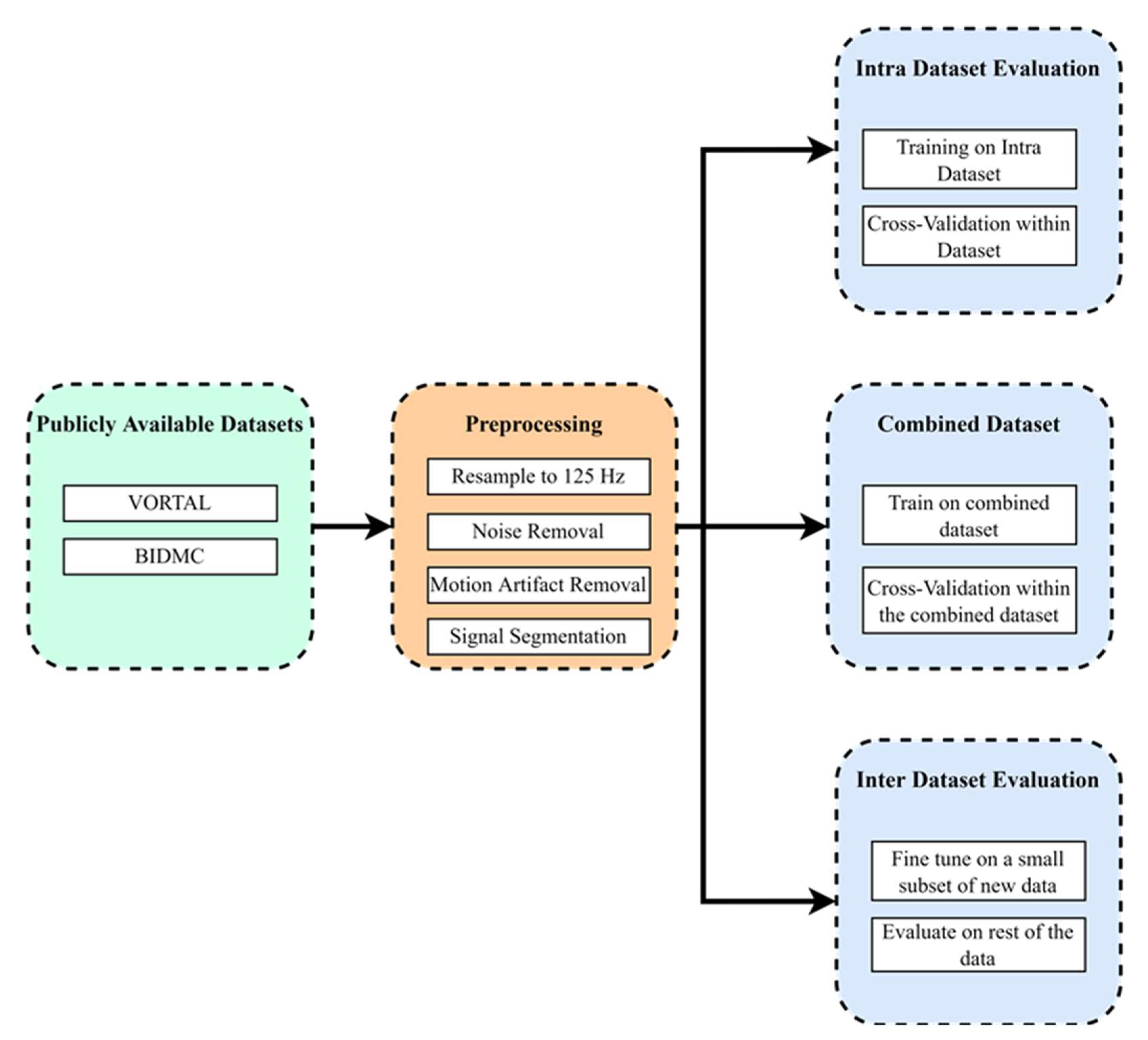
2. Materials and Methods
2.1. Preprocessing
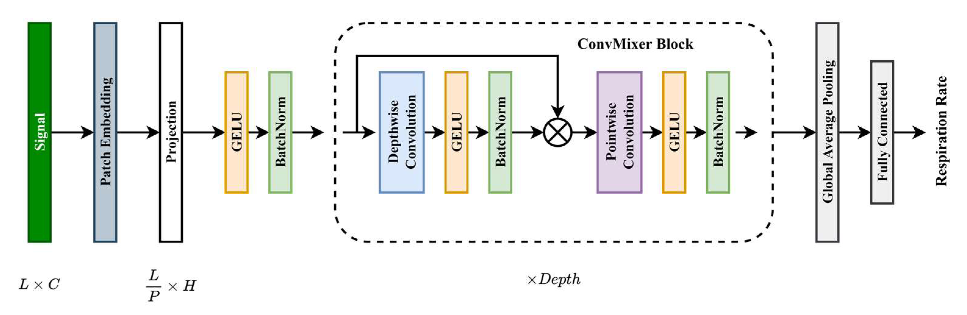
2.2. Neural Network Architectures
2.3. Dataset Description
2.4. Training Methodology
2.5. Evaluation Criteria
- Mean absolute error (MAE): MAE is the average of the absolute errors. This is one of the standard metrics for regression problems.
- RMSE (root mean squared error): RMSE is the square root of the mean of squared errors. This metric is very harsh when the predictions and ground truth differ largely.
- Correlation coefficient (R): R is used to calculate the degree to which two variables (prediction and ground truth) are linked. This is a scale-invariant metric that allows for reliable comparison between multiple datasets.where MSE (baseline) =
- 2SD: Standard deviation (SD) is a statistical technique that measures the spread of data relative to its mean. 2SD is significant as it indicates the 95% confidence interval.where error =
- Limit of agreement (LOA): LOA allows for errors resulting from random and systematic events. Hence, it is helpful to assess the reliability of the predictions of the models. In this work, 95% LOAs were calculated.
3. Results and Discussion
3.1. Intra Dataset Evaluation
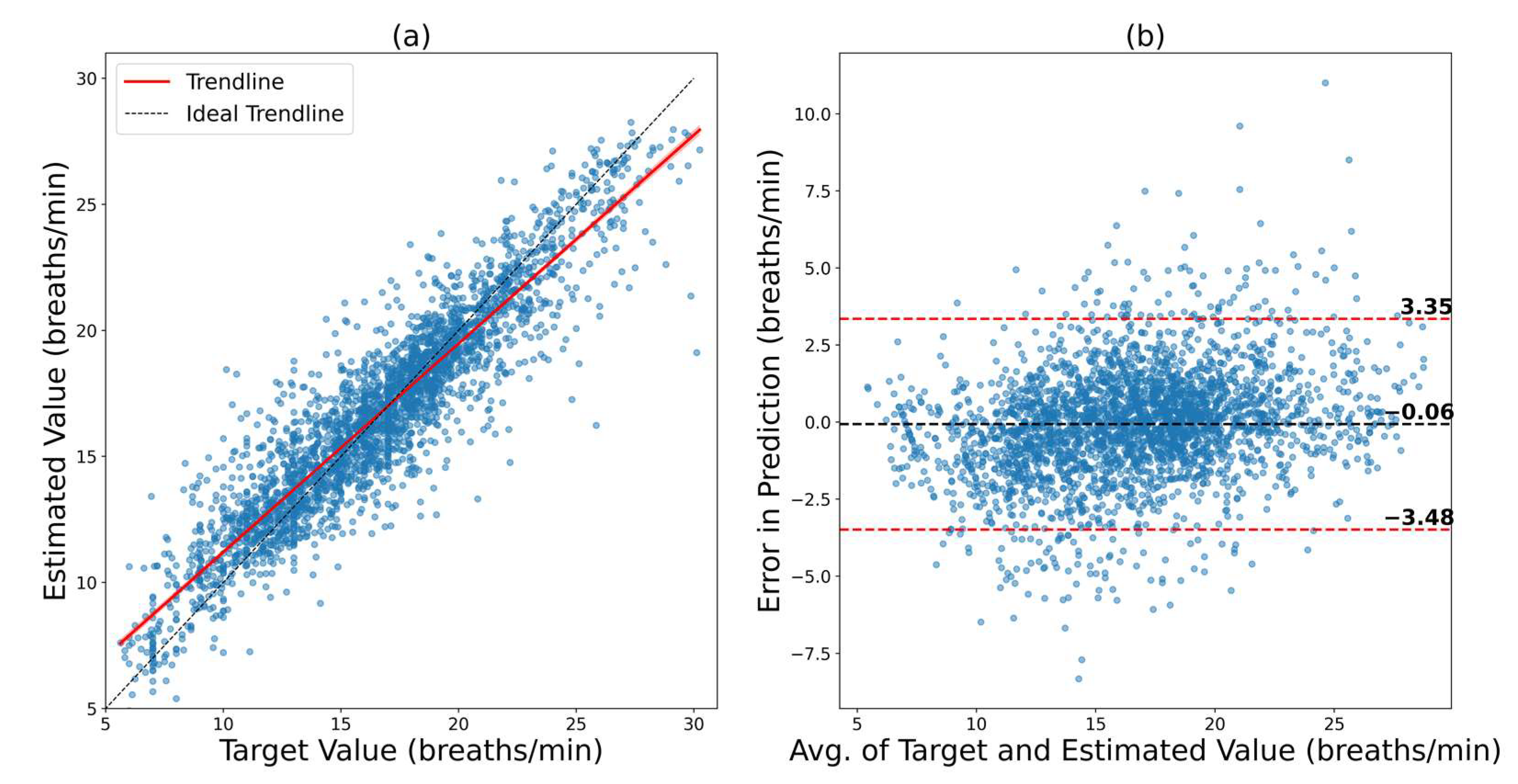
3.1.1. VORTAL
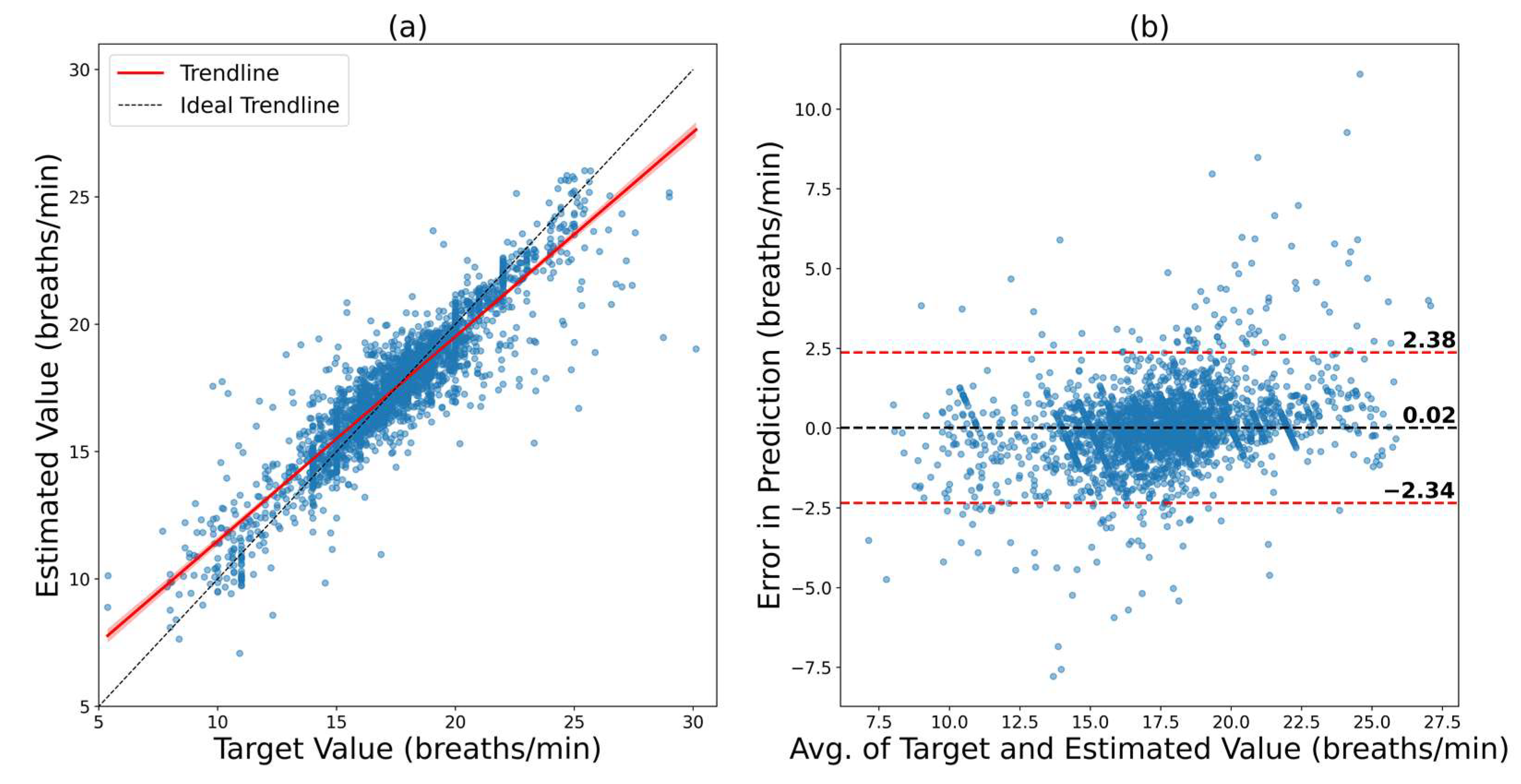
3.1.2. BIDMC
3.2. Inter Dataset Evaluation
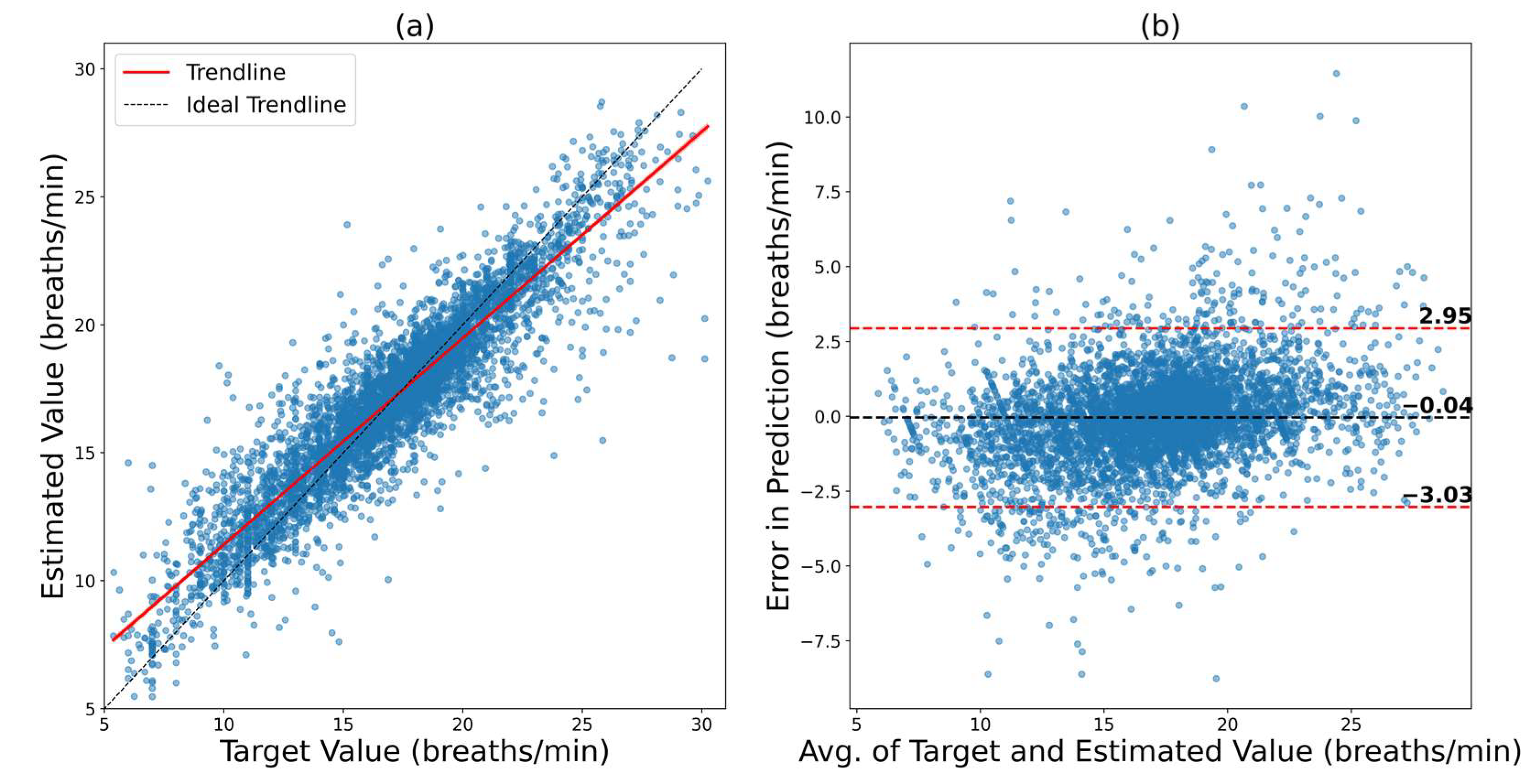
3.2.1. Combined Dataset
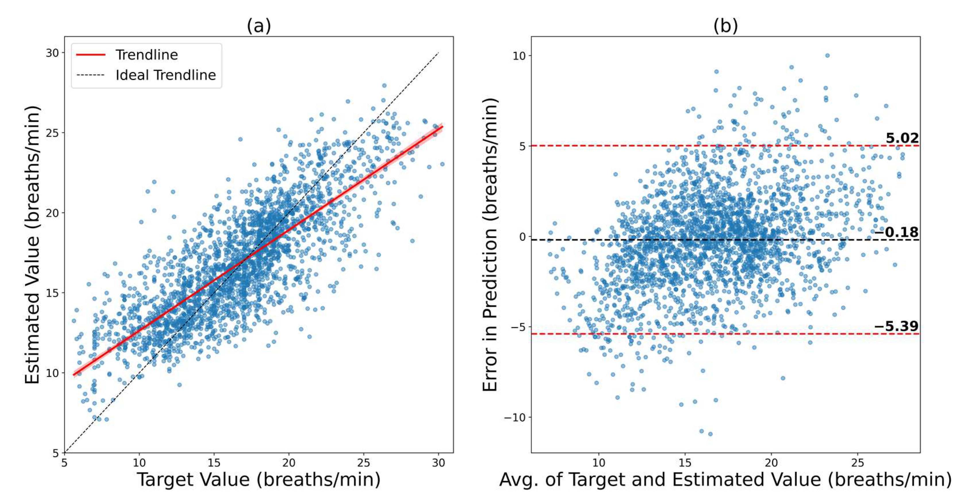
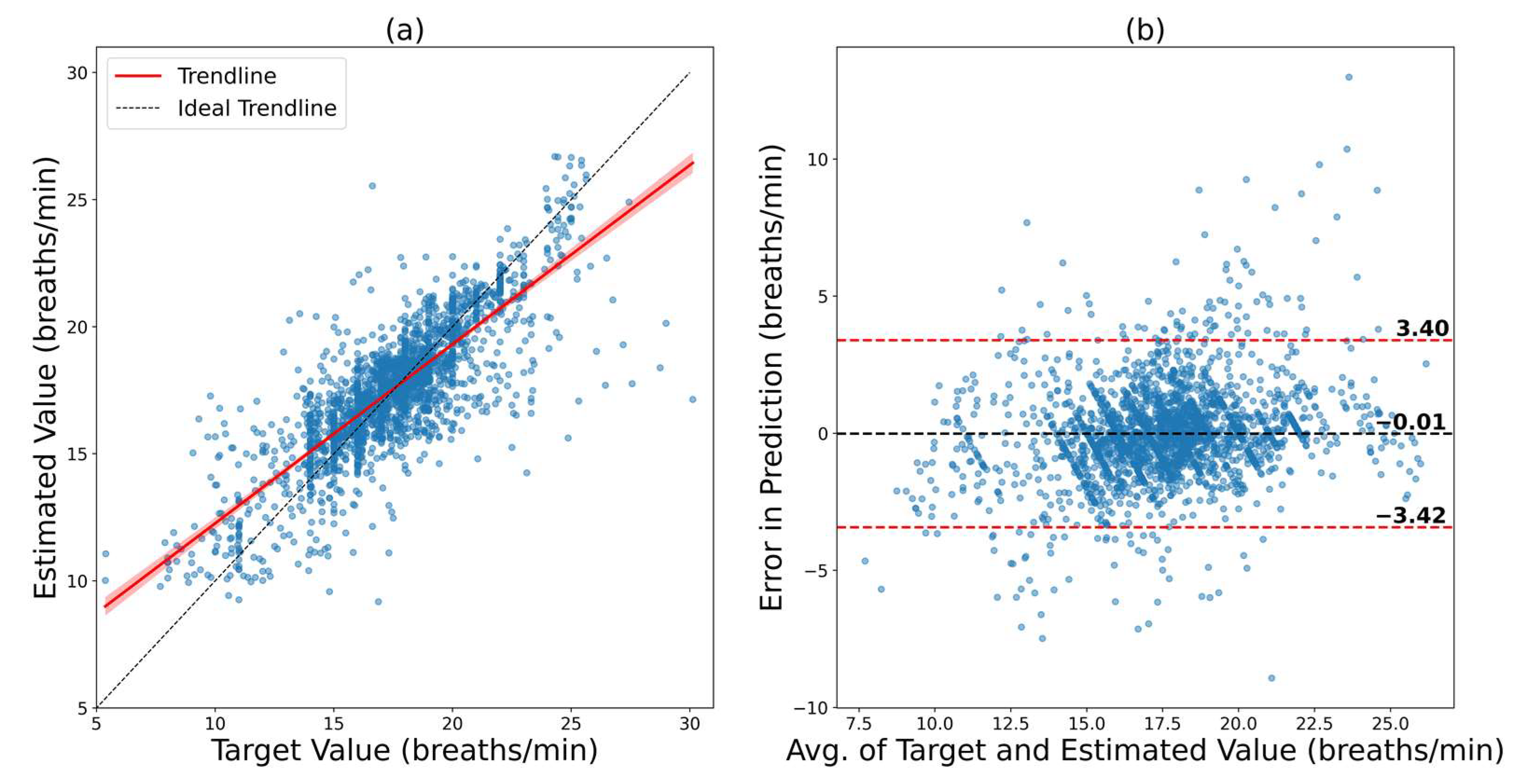
3.2.2. Fine-Tuning on a Small Subset of the New Dataset
3.3. Comparison with Literature
4. Conclusions
Supplementary Materials
Author Contributions
Funding
Institutional Review Board Statement
Informed Consent Statement
Data Availability Statement
Conflicts of Interest
References
- Fieselmann, J.F.; Hendryx, M.S.; Helms, C.M.; Wakefield, D.S. Respiratory Rate Predicts Cardiopulmonary Arrest for Internal Medicine Inpatients. J. Gen. Intern. Med. 1993, 8, 354–360. [Google Scholar] [CrossRef] [PubMed]
- Goldhill, D.R.; White, S.A.; Sumner, A. Physiological Values and Procedures in the 24 h before ICU Admission from the Ward. Anaesthesia 1999, 54, 529–534. [Google Scholar] [CrossRef] [PubMed]
- Ebell, M.H. Predicting Pneumonia in Adults with Respiratory Illness. Am. Fam. Physician 2007, 76, 560. [Google Scholar] [PubMed]
- Gravelyn, T.R.; Weg, J.G. Respiratory Rate as an Indicator of Acute Respiratory Dysfunction. JAMA 1980, 244, 1123–1125. [Google Scholar] [CrossRef] [PubMed]
- Schein, R.M.H.; Hazday, N.; Pena, M.; Ruben, B.H.; Sprung, C.L. Clinical Antecedents to In-Hospital Cardiopulmonary Arrest. Chest 1990, 98, 1388–1392. [Google Scholar] [CrossRef] [PubMed]
- Duckitt, R.W.; Buxton-Thomas, R.; Walker, J.; Cheek, E.; Bewick, V.; Venn, R.; Forni, L.G. Worthing Physiological Scoring System: Derivation and Validation of a Physiological Early-Warning System for Medical Admissions. An Observational, Population-Based Single-Centre Study. Br. J. Anaesth. 2007, 98, 769–774. [Google Scholar] [CrossRef] [PubMed]
- Karlen, W.; Raman, S.; Ansermino, J.M.; Dumont, G.A. Multiparameter Respiratory Rate Estimation from the Photoplethysmogram. IEEE Trans. Biomed. Eng. 2013, 60, 1946–1953. [Google Scholar] [CrossRef]
- Khalil, A.; Kelen, G.; Rothman, R.E. A Simple Screening Tool for Identification of Community-Acquired Pneumonia in an Inner City Emergency Department. Emerg. Med. J. 2007, 24, 336–338. [Google Scholar] [CrossRef]
- Pimentel, M.A.F.; Charlton, P.H.; Clifton, D.A. Probabilistic Estimation of Respiratory Rate from Wearable Sensors. In Wearable Electronics Sensors; Springer: Berlin/Heidelberg, Germany, 2015; pp. 241–262. [Google Scholar]
- Goldhaber, S.Z.; Visani, L.; De Rosa, M. Acute Pulmonary Embolism: Clinical Outcomes in the International Cooperative Pulmonary Embolism Registry (ICOPER). Lancet 1999, 353, 1386–1389. [Google Scholar] [CrossRef]
- Cretikos, M.A.; Bellomo, R.; Hillman, K.; Chen, J.; Finfer, S.; Flabouris, A. Respiratory Rate: The Neglected Vital Sign. Med. J. Aust. 2008, 188, 657–659. [Google Scholar] [CrossRef]
- Farrohknia, N.; Castrén, M.; Ehrenberg, A.; Lind, L.; Oredsson, S.; Jonsson, H.; Asplund, K.; Göransson, K.E. Emergency Department Triage Scales and Their Components: A Systematic Review of the Scientific Evidence. Scand. J. Trauma. Resusc. Emerg. Med. 2011, 19, 42. [Google Scholar] [CrossRef]
- Miller, D.J.; Capodilupo, J.V.; Lastella, M.; Sargent, C.; Roach, G.D.; Lee, V.H.; Capodilupo, E.R. Analyzing Changes in Respiratory Rate to Predict the Risk of COVID-19 Infection. PLoS ONE 2020, 15, e0243693. [Google Scholar] [CrossRef]
- Rahman, T.; Akinbi, A.; Chowdhury, M.E.H.; Rashid, T.A.; Sengür, A.; Khandakar, A.; Islam, K.R.; Ismael, A.M. COV-ECGNET: COVID-19 Detection Using ECG Trace Images with Deep Convolutional Neural Network. Heal. Inf. Sci. Syst. 2022, 10, 1–16. [Google Scholar] [CrossRef]
- Cretikos, M.; Chen, J.; Hillman, K.; Bellomo, R.; Finfer, S.; Flabouris, A.; Investigators, M.S. The Objective Medical Emergency Team Activation Criteria: A Case--Control Study. Resuscitation 2007, 73, 62–72. [Google Scholar] [CrossRef]
- William, B.; Albert, G.; Ball, C.; Bell, D.; Binks, R.; Durham, L.; Eddleston, J.; Edwards, N.; Evans, D.; Jones, M.; et al. National Early Warning Score (NEWS): Standardizing the Assessment of Acute Illness Severity in the NHS. Rep. Work. Party 2012, 12, 501–503. [Google Scholar]
- Lovett, P.B.; Buchwald, J.M.; Stürmann, K.; Bijur, P. The Vexatious Vital: Neither Clinical Measurements by Nurses nor an Electronic Monitor Provides Accurate Measurements of Respiratory Rate in Triage. Ann. Emerg. Med. 2005, 45, 68–76. [Google Scholar] [CrossRef]
- Philip, K.E.J.; Pack, E.; Cambiano, V.; Rollmann, H.; Weil, S.; O’Beirne, J. The Accuracy of Respiratory Rate Assessment by Doctors in a London Teaching Hospital: A Cross-Sectional Study. J. Clin. Monit. Comput. 2015, 29, 455–460. [Google Scholar] [CrossRef]
- Jaffe, M.B. Infrared Measurement of Carbon Dioxide in the Human Breath:“Breathe-through” Devices from Tyndall to the Present Day. Anesth. Analg. 2008, 107, 890–904. [Google Scholar] [CrossRef]
- Chowdhury, M.H.; Shuzan, M.N.I.; Chowdhury, M.E.H.; Mahbub, Z.B.; Uddin, M.M.; Khandakar, A.; Reaz, M.B.I. Estimating Blood Pressure from the Photoplethysmogram Signal and Demographic Features Using Machine Learning Techniques. Sensors 2020, 20, 3127. [Google Scholar] [CrossRef]
- Chowdhury, M.E.H.; Alzoubi, K.; Khandakar, A.; Khallifa, R.; Abouhasera, R.; Koubaa, S.; Ahmed, R.; Hasan, A. Wearable Real-Time Heart Attack Detection and Warning System to Reduce Road Accidents. Sensors 2019, 19, 2780. [Google Scholar] [CrossRef]
- Ibtehaz, N.; Chowdhury, M.E.H.; Khandakar, A.; Kiranyaz, S.; Rahman, M.S.; Tahir, A.; Qiblawey, Y.; Rahman, T. EDITH: ECG Biometrics Aided by Deep Learning for Reliable Individual AuTHentication. IEEE Trans. Emerg. Top. Comput. Intell. 2021. [Google Scholar] [CrossRef]
- Shen, Y.; Voisin, M.; Aliamiri, A.; Avati, A.; Hannun, A.; Ng, A. Ambulatory Atrial Fibrillation Monitoring Using Wearable Photoplethysmography with Deep Learning. In Proceedings of the 25th ACM SIGKDD International Conference on Knowledge Discovery & Data Mining, Anchorage, AK, USA, 4–8 August 2019; pp. 1909–1916. [Google Scholar]
- Adochiei, N.I.; David, V.; Tudosa, I. Methods of Electromagnetic Interference Reduction in Electrocardiographic Signal Acquisition. Environ. Eng. Manag. J. 2011, 10, 553–559. [Google Scholar] [CrossRef]
- Moody, G.B.; Mark, R.G.; Zoccola, A.; Mantero, S. Derivation of Respiratory Signals from Multi-Lead ECGs. Comput. Cardiol. 1985, 12, 113–116. [Google Scholar]
- Orphanidou, C.; Fleming, S.; Shah, S.A.; Tarassenko, L. Data Fusion for Estimating Respiratory Rate from a Single-Lead ECG. Biomed. Signal Process. Control 2013, 8, 98–105. [Google Scholar] [CrossRef]
- Mirmohamadsadeghi, L.; Vesin, J.-M. Respiratory Rate Estimation from the ECG Using an Instantaneous Frequency Tracking Algorithm. Biomed. Signal Process. Control 2014, 14, 66–72. [Google Scholar] [CrossRef]
- Drew, B.J.; Harris, P.; Zègre-Hemsey, J.K.; Mammone, T.; Schindler, D.; Salas-Boni, R.; Bai, Y.; Tinoco, A.; Ding, Q.; Hu, X. Insights into the Problem of Alarm Fatigue with Physiologic Monitor Devices: A Comprehensive Observational Study of Consecutive Intensive Care Unit Patients. PLoS ONE 2014, 9, e110274. [Google Scholar] [CrossRef]
- Charlton, P.H.; Birrenkott, D.A.; Bonnici, T.; Pimentel, M.A.F.; Johnson, A.E.W.; Alastruey, J.; Tarassenko, L.; Watkinson, P.J.; Beale, R.; Clifton, D.A. Breathing Rate Estimation from the Electrocardiogram and Photoplethysmogram: A Review. IEEE Rev. Biomed. Eng. 2017, 11, 2–20. [Google Scholar] [CrossRef]
- Charlton, P.H.; Bonnici, T.; Tarassenko, L.; Clifton, D.A.; Beale, R.; Watkinson, P.J. An Assessment of Algorithms to Estimate Respiratory Rate from the Electrocardiogram and Photoplethysmogram. Physiol. Meas. 2016, 37, 610. [Google Scholar] [CrossRef]
- Charlton, P.H.; Bonnici, T.; Tarassenko, L.; Alastruey, J.; Clifton, D.A.; Beale, R.; Watkinson, P.J. Extraction of Respiratory Signals from the Electrocardiogram and Photoplethysmogram: Technical and Physiological Determinants. Physiol. Meas. 2017, 38, 669. [Google Scholar] [CrossRef]
- Shah, S.A.; Fleming, S.; Thompson, M.; Tarassenko, L. Respiratory Rate Estimation during Triage of Children in Hospitals. J. Med. Eng. Technol. 2015, 39, 514–524. [Google Scholar]
- Zhang, X.; Ding, Q. Respiratory Rate Estimation from the Photoplethysmogram via Joint Sparse Signal Reconstruction and Spectra Fusion. Biomed. Signal Process. Control 2017, 35, 1–7. [Google Scholar] [CrossRef]
- Pirhonen, M.; Peltokangas, M.; Vehkaoja, A. Acquiring Respiration Rate from Photoplethysmographic Signal by Recursive Bayesian Tracking of Intrinsic Modes in Time-Frequency Spectra. Sensors 2018, 18, 1693. [Google Scholar] [CrossRef] [PubMed]
- Jarchi, D.; Rodgers, S.J.; Tarassenko, L.; Clifton, D.A. Accelerometry-Based Estimation of Respiratory Rate for Post-Intensive Care Patient Monitoring. IEEE Sens. J. 2018, 18, 4981–4989. [Google Scholar] [CrossRef]
- Hartmann, V.; Liu, H.; Chen, F.; Hong, W.; Hughes, S.; Zheng, D. Towards Accurate Extraction of Respiratory Frequency from the Photoplethysmogram: Effect of Measurement Site. Front. Physiol. 2019, 10, 732. [Google Scholar] [CrossRef] [PubMed]
- L’Her, E.; N’Guyen, Q.-T.; Pateau, V.; Bodenes, L.; Lellouche, F. Photoplethysmographic Determination of the Respiratory Rate in Acutely Ill Patients: Validation of a New Algorithm and Implementation into a Biomedical Device. Ann. Intensive Care 2019, 9, 11. [Google Scholar] [CrossRef] [PubMed]
- Motin, M.A.; Karmakar, C.K.; Palaniswami, M. Selection of Empirical Mode Decomposition Techniques for Extracting Breathing Rate from PPG. IEEE Signal Process. Lett. 2019, 26, 592–596. [Google Scholar] [CrossRef]
- Motin, M.A.; Kumar Karmakar, C.; Kumar, D.K.; Palaniswami, M. PPG Derived Respiratory Rate Estimation in Daily Living Conditions. Proc. Annu. Int. Conf. IEEE Eng. Med. Biol. Soc. EMBS 2020, 2020, 2736–2739. [Google Scholar] [CrossRef]
- Rathore, K.S.; Vijayarangan, S.; SP, P.; Sivaprakasam, M. A Deep Learning Based Multitask Network for Respiration Rate Estimation--A Practical Perspective. arXiv 2021, arXiv:2112.09071. [Google Scholar]
- Lampier, L.C.; Coelho, Y.L.; Caldeira, E.M.O.; Bastos-Filho, T.F. A Deep Learning Approach to Estimate the Respiratory Rate from Photoplethysmogram. Ingenius 2022, 96–104. [Google Scholar] [CrossRef]
- Pimentel, M.A.F.; Johnson, A.E.W.; Charlton, P.H.; Birrenkott, D.; Watkinson, P.J.; Tarassenko, L.; Clifton, D.A. Toward a Robust Estimation of Respiratory Rate from Pulse Oximeters. IEEE Trans. Biomed. Eng. 2016, 64, 1914–1923. [Google Scholar] [CrossRef]
- Shuzan, M.N.I.; Chowdhury, M.H.; Hossain, M.S.; Chowdhury, M.E.H.; Reaz, M.B.I.; Uddin, M.M.; Khandakar, A.; Bin Mahbub, Z.; Ali, S.H.M. A Novel Non-Invasive Estimation of Respiration Rate from Motion Corrupted Photoplethysmograph Signal Using Machine Learning Model. IEEE Access 2021, 9, 96775–96790. [Google Scholar] [CrossRef]
- Chatterjee, A.; Roy, U.K. PPG Based Heart Rate Algorithm Improvement with Butterworth IIR Filter and Savitzky-Golay FIR Filter. In Proceedings of the 2018 2nd International Conference on Electronics, Materials Engineering & Nano-Technology (IEMENTech), Kolkata, India, 4–5 April 2018; 2018; pp. 1–6. [Google Scholar]
- Wang, Y.; Markert, R. Filter Bank Property of Variational Mode Decomposition and Its Applications. Signal Processing 2016, 120, 509–521. [Google Scholar] [CrossRef]
- Roy, B.; Gupta, R.; Chandra, J.K. Estimation of Respiration Rate from Motion Corrupted Photoplethysmogram: A Combined Time and Frequency Domain Approach. In Proceedings of the 2019 IEEE Region 10 Symposium (TENSYMP), Kolkata, India, 7–9 June 2019; 2019; pp. 292–297. [Google Scholar]
- He, K.; Zhang, X.; Ren, S.; Sun, J. Deep Residual Learning for Image Recognition. In Proceedings of the IEEE Conference on Computer Vision and Pattern Recognition, Las Vegas, NV, USA, 27–30 June 2016; IEEE: Manhattan, NY, USA, 2016; pp. 770–778. [Google Scholar]
- Huang, G.; Liu, Z.; Van Der Maaten, L.; Weinberger, K.Q. Densely Connected Convolutional Networks. In Proceedings of the IEEE Conference on Computer Vision and Pattern Recognition, Honolulu, HI, USA, 21–26 July 2017; IEEE: Manhattan, NY, USA, 2017; pp. 4700–4708. [Google Scholar]
- Szegedy, C.; Liu, W.; Jia, Y.; Sermanet, P.; Reed, S.; Anguelov, D.; Erhan, D.; Vanhoucke, V.; Rabinovich, A. Going Deeper with Convolutions. In Proceedings of the IEEE Conference on Computer Vision and Pattern Recognition, Boston, MA, USA, 7–12 June 2015; IEEE: Manhattan, NY, USA, 2015; pp. 1–9. [Google Scholar]
- Howard, A.G.; Zhu, M.; Chen, B.; Kalenichenko, D.; Wang, W.; Weyand, T.; Andreetto, M.; Adam, H. Mobilenets: Efficient Convolutional Neural Networks for Mobile Vision Applications. arXiv 2017, arXiv:1704.04861. [Google Scholar]
- Trockman, A.; Kolter, J.Z. Patches Are All You Need? arXiv 2022, arXiv:2201.09792. [Google Scholar]
- Saeed, M.; Villarroel, M.; Reisner, A.T.; Clifford, G.; Lehman, L.-W.; Moody, G.; Heldt, T.; Kyaw, T.H.; Moody, B.; Mark, R.G. Multiparameter Intelligent Monitoring in Intensive Care II (MIMIC-II): A Public-Access Intensive Care Unit Database. Crit. Care Med. 2011, 39, 952. [Google Scholar] [CrossRef]


| Median | Range | ||
|---|---|---|---|
| VORTAL | Sex (female) | 54% | - |
| Age (years) | 29 | 18–39 | |
| BMI (kg/m2) | 23 | - | |
| RR (bpm) | - | 5–32 | |
| PPG Sample Rate (Hz) | 500 | - | |
| BIDMC | Sex (female) | 60% | - |
| Age (years) | - | 19–90+ | |
| RR (bpm) | - | 5–25 | |
| PPG Sample Rate (Hz) | 125 | - | |
| Model | Parameters (Millions) | R | MAE (bpm) | RMSE (bpm) |
|---|---|---|---|---|
| Resnet18 | 0.93 | 0.6462 | 2.6926 | 3.4274 |
| Inception_v1 | 3.40 | 0.8239 | 1.8698 | 2.5463 |
| Mobilenet_v1 | 2.01 | 0.7349 | 2.4252 | 3.1651 |
| Densenet121 | 277.36 | 0.7494 | 2.2265 | 2.9825 |
| ConvMixer | 0.56 | 0.9209 | 1.2702 | 1.7450 |
| Scenario | R | RMSE (bpm) | MAE (bpm) | LOA (bpm) | 2SD (bpm) |
|---|---|---|---|---|---|
| Fivefold cross-validation on VORTAL | 0.9209 | 1.7450 | 1.2702 | −3.48 to 3.35 | 3.42 |
| Fivefold cross-validation on BIDMC | 0.9155 | 1.2039 | 0.7656 | −2.34 to 2.38 | 2.36 |
| Fivefold cross-validation on the combined dataset | 0.9183 | 1.5246 | 1.0417 | −3.03 to 2.95 | 2.99 |
| BIDMC model fine-tuned on VORTAL | 0.8017 | 2.6609 | 2.0174 | −5.39 to 5.02 | 5.21 |
| VORTAL model fine-tuned on BIDMC | 0.8123 | 1.7403 | 1.1838 | −3.42 to 3.40 | 3.41 |
| Author | Database | Subject | Method | Metric | Result |
|---|---|---|---|---|---|
| Pirhonenet al. [34] | Vortal | 39 | Wavelet Synchro squeezing Transform | MAE RMSE R 2SD | 2.33 3.68 - - |
| Jarchiet al. [35] | BIDMC | 10 | Accelerometer | MAE RMSE R 2SD | 2.56 - - - |
| Shuzanet al. [43] | Vortal | 39 | Machine Learning | MAE RMSE R 2SD | 1. 97 2.63 0.88 5.25 |
| Lampieret al. [41] | BIDMC | 53 | Deep Neural Network | MAE RMSE R 2SD | 3.4 6.9 - - |
| This work (Intra Dataset) | Vortal | 39 | ConvMixer | MAE RMSE R 2SD | 1.27 1.75 0.92 3.42 |
| This work (Intra Dataset) | BIDMC | 53 | ConvMixer | MAE RMSE R 2SD | 0.77 1.20 0.92 2.36 |
Publisher’s Note: MDPI stays neutral with regard to jurisdictional claims in published maps and institutional affiliations. |
© 2022 by the authors. Licensee MDPI, Basel, Switzerland. This article is an open access article distributed under the terms and conditions of the Creative Commons Attribution (CC BY) license (https://creativecommons.org/licenses/by/4.0/).
Share and Cite
Chowdhury, M.H.; Shuzan, M.N.I.; Chowdhury, M.E.H.; Reaz, M.B.I.; Mahmud, S.; Al Emadi, N.; Ayari, M.A.; Ali, S.H.M.; Bakar, A.A.A.; Rahman, S.M.; et al. Lightweight End-to-End Deep Learning Solution for Estimating the Respiration Rate from Photoplethysmogram Signal. Bioengineering 2022, 9, 558. https://doi.org/10.3390/bioengineering9100558
Chowdhury MH, Shuzan MNI, Chowdhury MEH, Reaz MBI, Mahmud S, Al Emadi N, Ayari MA, Ali SHM, Bakar AAA, Rahman SM, et al. Lightweight End-to-End Deep Learning Solution for Estimating the Respiration Rate from Photoplethysmogram Signal. Bioengineering. 2022; 9(10):558. https://doi.org/10.3390/bioengineering9100558
Chicago/Turabian StyleChowdhury, Moajjem Hossain, Md Nazmul Islam Shuzan, Muhammad E. H. Chowdhury, Mamun Bin Ibne Reaz, Sakib Mahmud, Nasser Al Emadi, Mohamed Arselene Ayari, Sawal Hamid Md Ali, Ahmad Ashrif A. Bakar, Syed Mahfuzur Rahman, and et al. 2022. "Lightweight End-to-End Deep Learning Solution for Estimating the Respiration Rate from Photoplethysmogram Signal" Bioengineering 9, no. 10: 558. https://doi.org/10.3390/bioengineering9100558
APA StyleChowdhury, M. H., Shuzan, M. N. I., Chowdhury, M. E. H., Reaz, M. B. I., Mahmud, S., Al Emadi, N., Ayari, M. A., Ali, S. H. M., Bakar, A. A. A., Rahman, S. M., & Khandakar, A. (2022). Lightweight End-to-End Deep Learning Solution for Estimating the Respiration Rate from Photoplethysmogram Signal. Bioengineering, 9(10), 558. https://doi.org/10.3390/bioengineering9100558