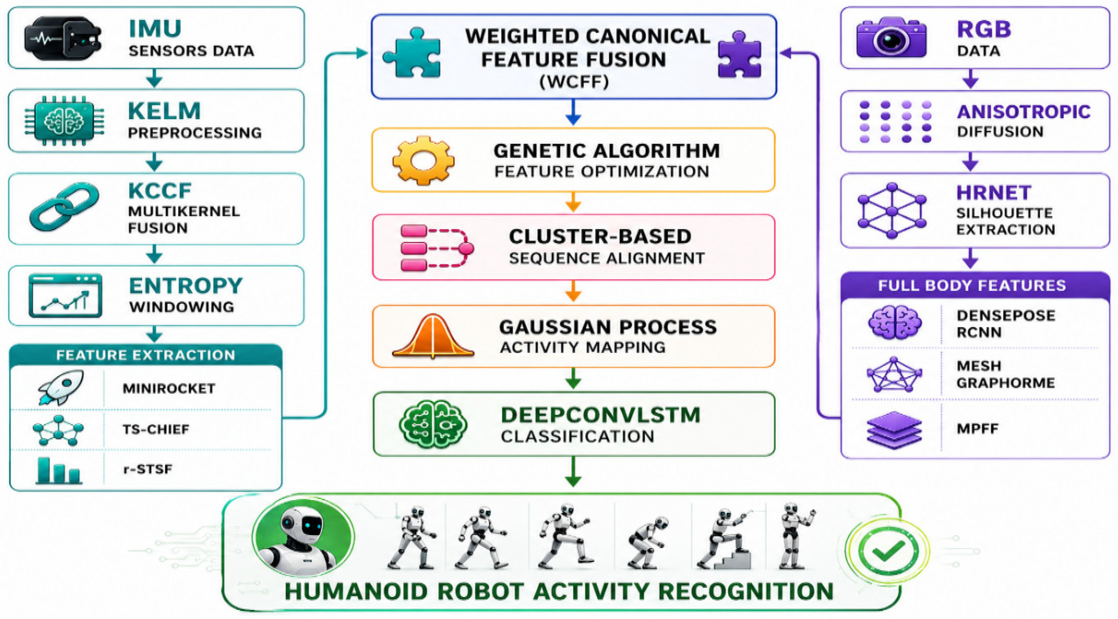
Figure 1.
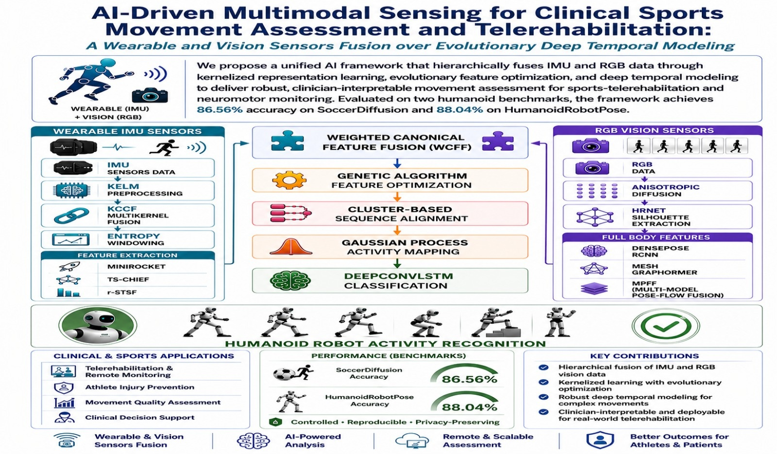
End-to-end pipeline of the proposed multimodal humanoid robotic activity recognition framework. Arrows represent the workflow between successive processing stages, and the different colors are used solely to differentiate the modules visually.
Figure 1.
End-to-end pipeline of the proposed multimodal humanoid robotic activity recognition framework. Arrows represent the workflow between successive processing stages, and the different colors are used solely to differentiate the modules visually.
Figure 2.
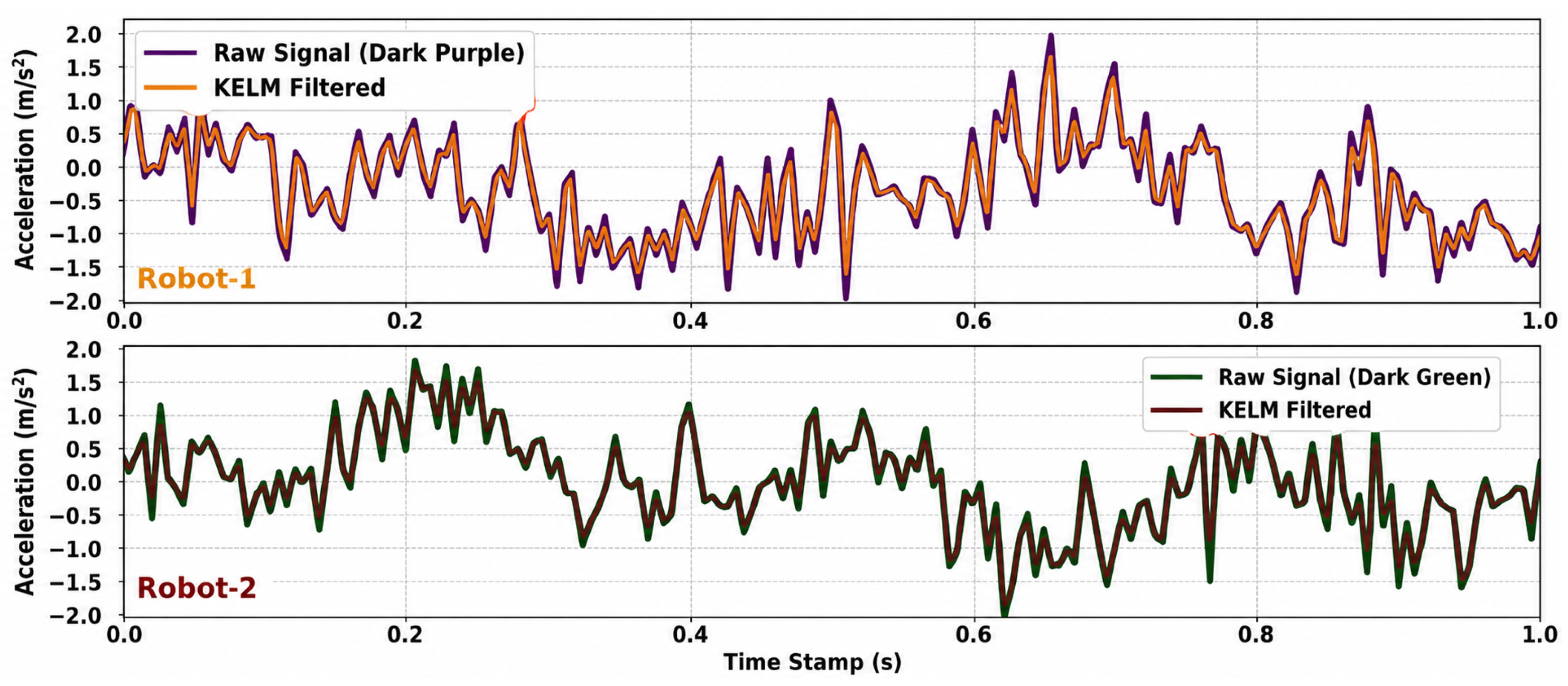
Effect of KELM-based preprocessing on a representative humanoid IMU acceleration channel: raw vs. denoised waveform.
Figure 2.
Effect of KELM-based preprocessing on a representative humanoid IMU acceleration channel: raw vs. denoised waveform.
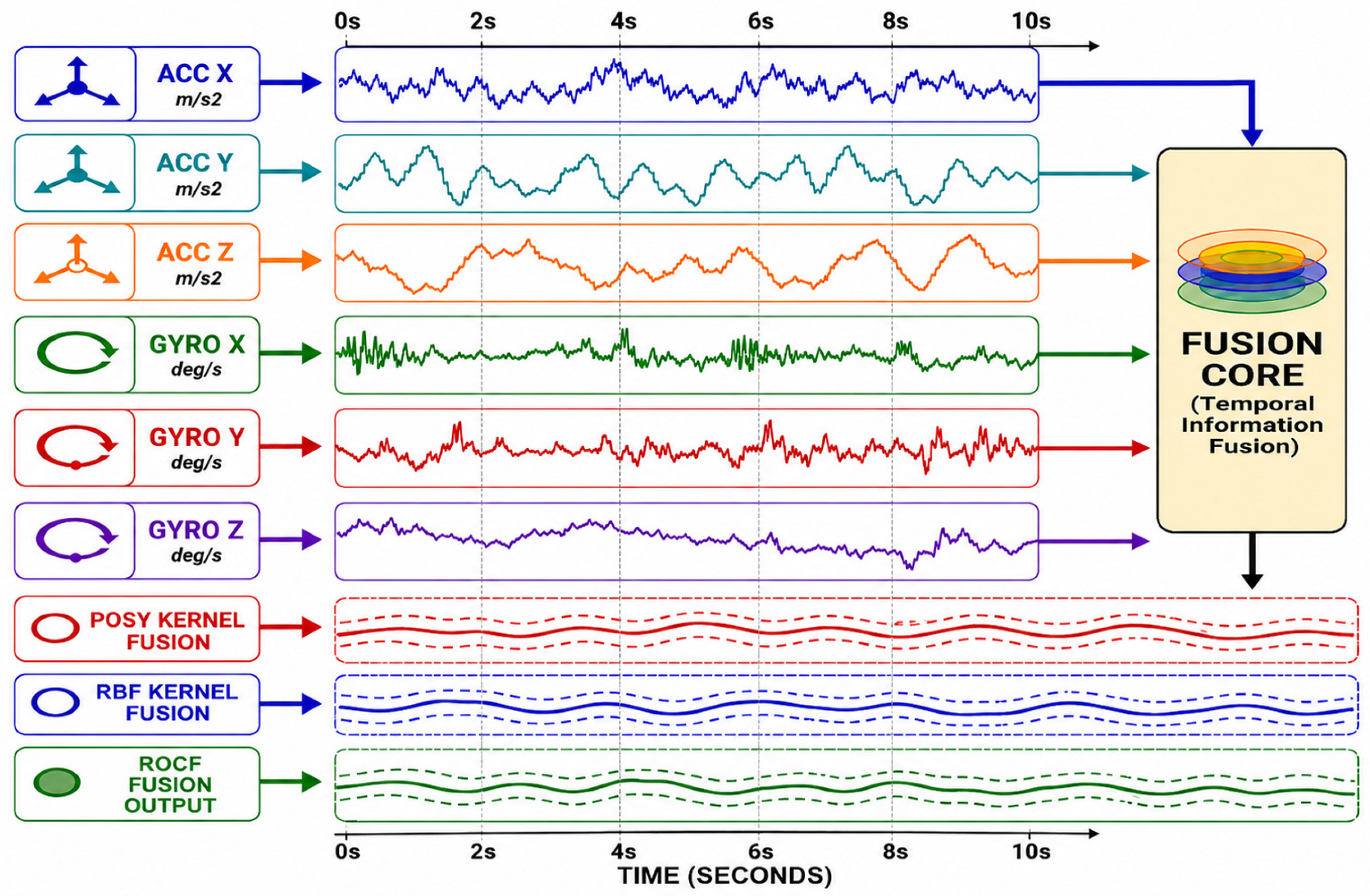
Figure 3.
Kernelized Canonical Correlation Fusion (KCCF) of tri-axial accelerometer and gyroscope signals using RBF and Polynomial kernels. Arrows indicate the data flow, solid and dashed lines represent fused signals and their confidence bounds, respectively, while colors distinguish sensor channels and fusion stages.
Figure 3.
Kernelized Canonical Correlation Fusion (KCCF) of tri-axial accelerometer and gyroscope signals using RBF and Polynomial kernels. Arrows indicate the data flow, solid and dashed lines represent fused signals and their confidence bounds, respectively, while colors distinguish sensor channels and fusion stages.
Figure 4.
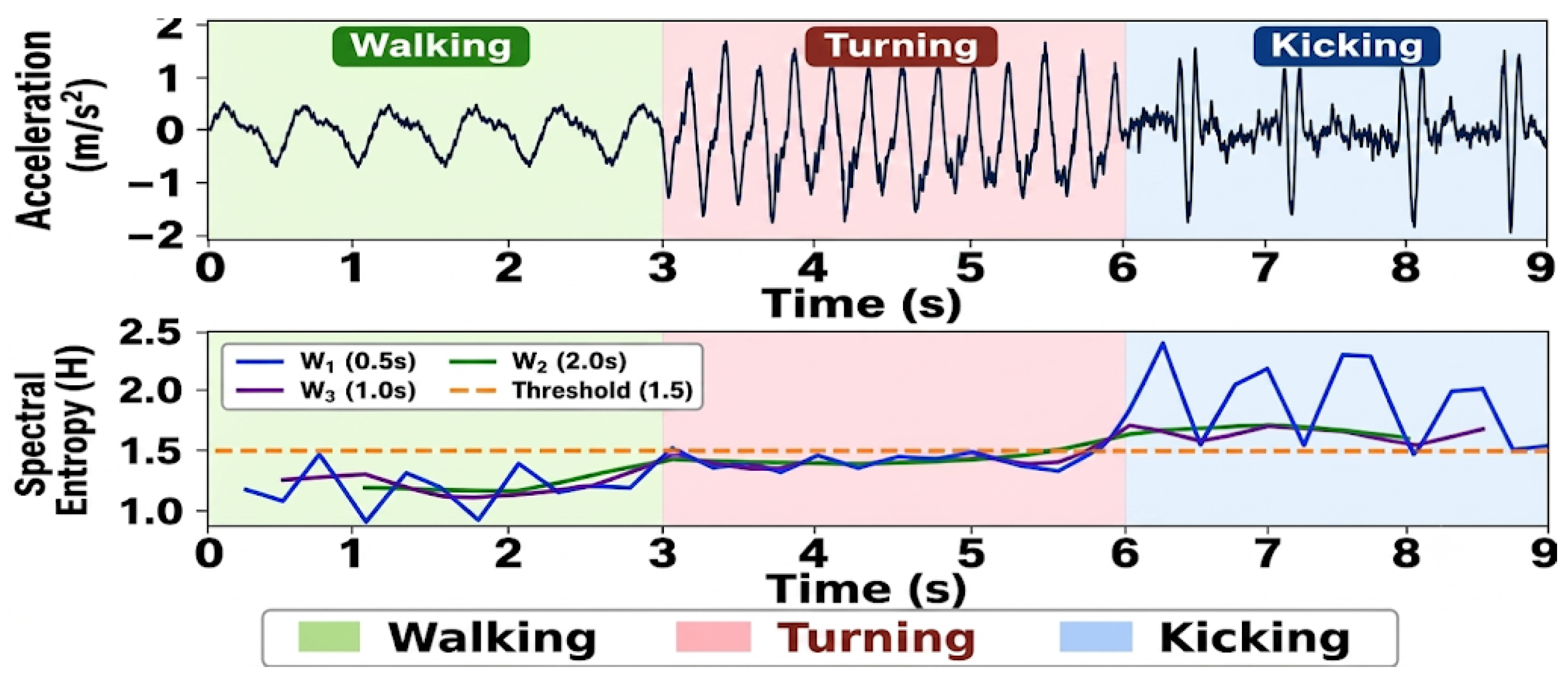
Multi-windowing segmentation via entropy monitoring, illustrating signal transitions between walking, running, and kicking based on spectral entropy thresholds.
Figure 4.
Multi-windowing segmentation via entropy monitoring, illustrating signal transitions between walking, running, and kicking based on spectral entropy thresholds.
Figure 5.
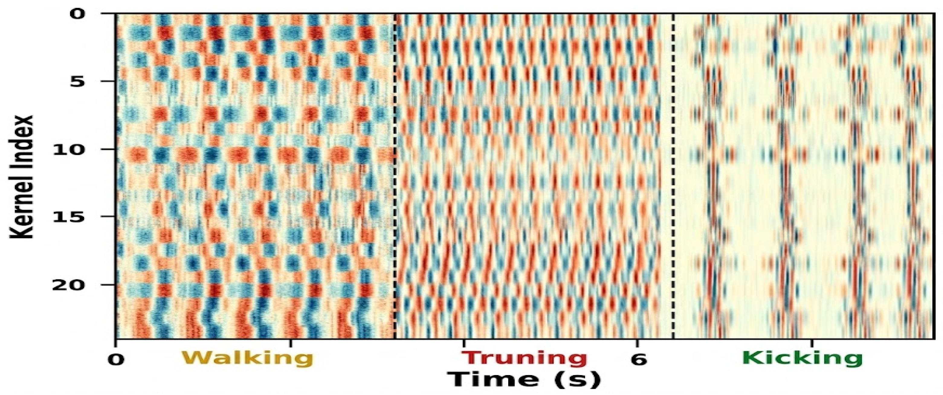
Heatmap of kernel-indexed features over time.
Figure 5.
Heatmap of kernel-indexed features over time.
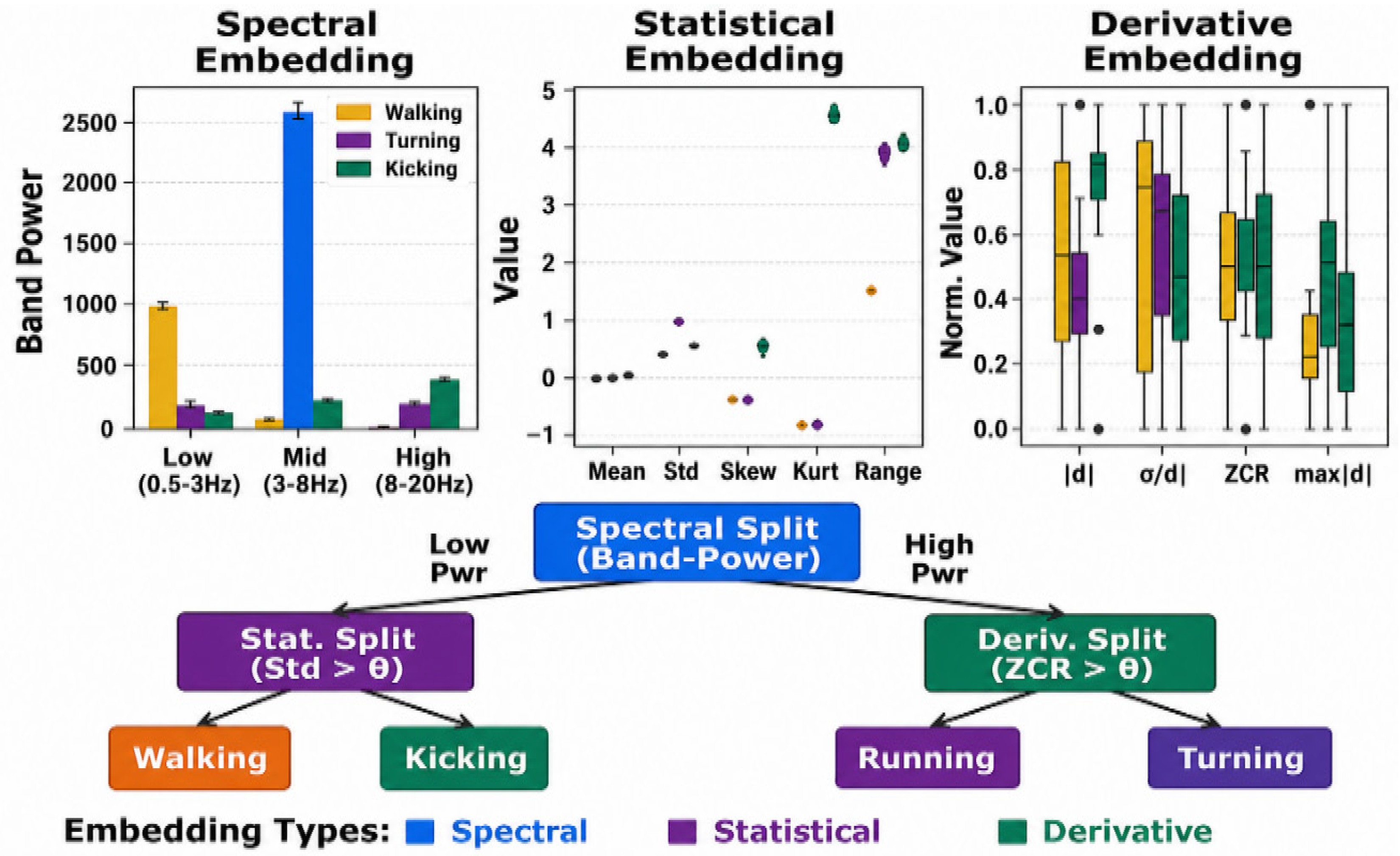
Figure 6.
TS–CHIEF heterogeneous embedding forest feature extraction across spectral, statistical, and derivative domains with its corresponding hierarchical decision structure for activity classification. Colors indicate the different embedding types and their associated activity classes.
Figure 6.
TS–CHIEF heterogeneous embedding forest feature extraction across spectral, statistical, and derivative domains with its corresponding hierarchical decision structure for activity classification. Colors indicate the different embedding types and their associated activity classes.
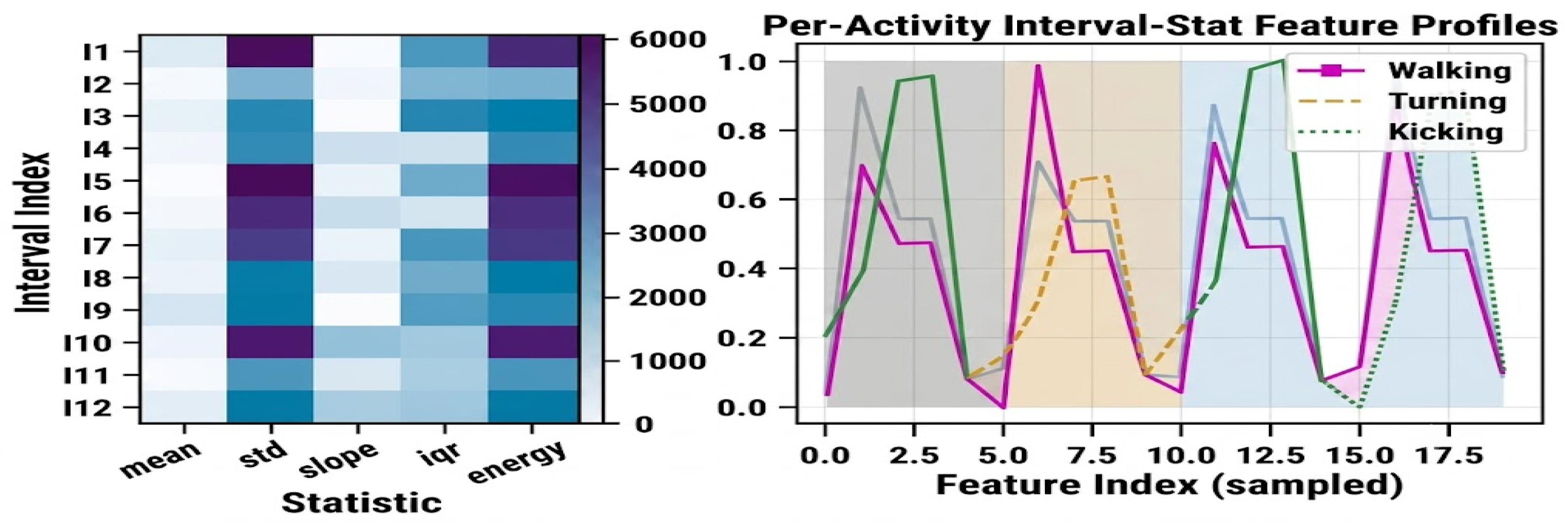
Figure 7.
Heatmap of statistical F-values and corresponding per-activity interval feature profiles for walking, turning, and kicking. Colours and line styles distinguish the activity profiles, while the green solid line denotes the overall top-ranked interval profile.
Figure 7.
Heatmap of statistical F-values and corresponding per-activity interval feature profiles for walking, turning, and kicking. Colours and line styles distinguish the activity profiles, while the green solid line denotes the overall top-ranked interval profile.
Figure 8.
Anisotropic diffusion preprocessing on an edge-preserving denoised output of an RGB frame.
Figure 8.
Anisotropic diffusion preprocessing on an edge-preserving denoised output of an RGB frame.
Figure 9.
Visual setup for multi-robot silhouette extraction and segmentation using HRNet.
Figure 9.
Visual setup for multi-robot silhouette extraction and segmentation using HRNet.
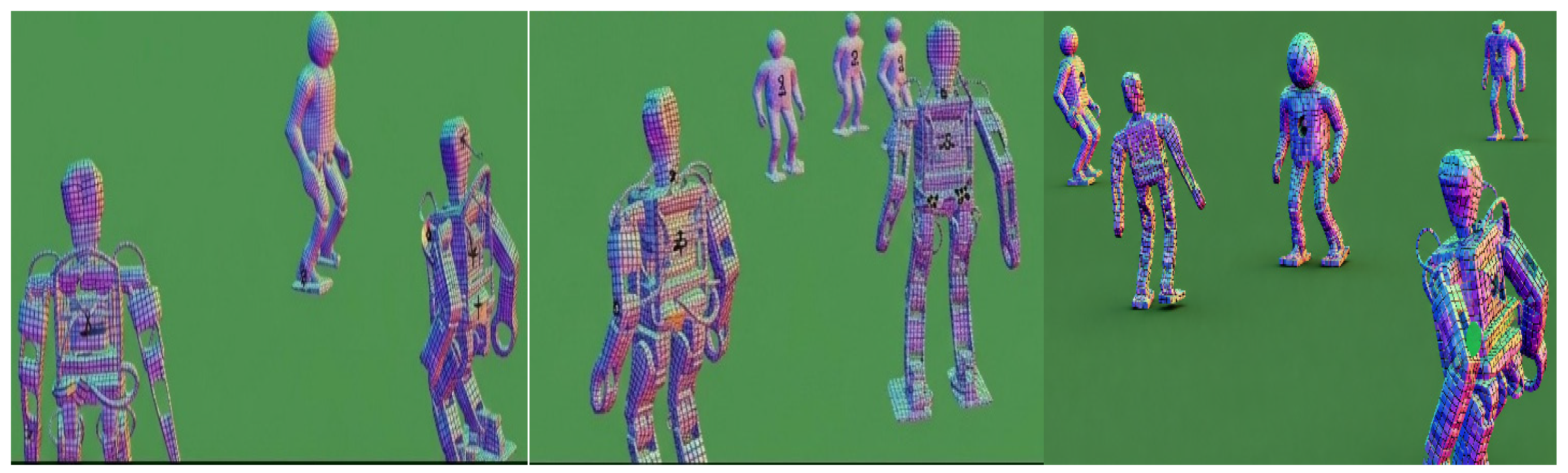
Figure 10.
DensePose R-CNN surface mapping. Dense 3D mesh estimation and UV coordinate mapping on the humanoid robot subjects.
Figure 10.
DensePose R-CNN surface mapping. Dense 3D mesh estimation and UV coordinate mapping on the humanoid robot subjects.
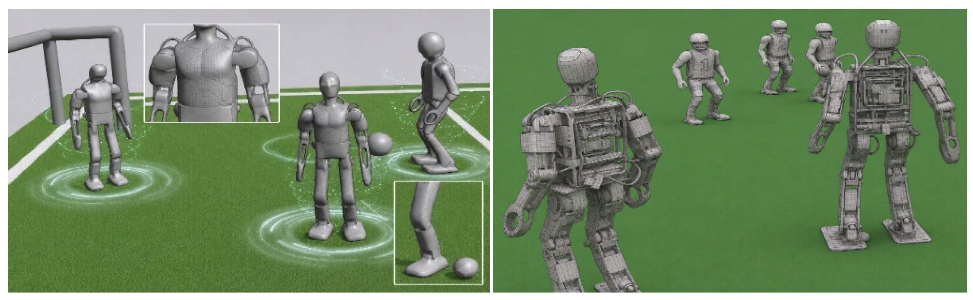
Figure 11.
3D human mesh generation with fine-grained body shape and pose modeling for activity analysis. Inset frames highlight enlarged views of selected body regions for enhanced visualization of pose details.
Figure 11.
3D human mesh generation with fine-grained body shape and pose modeling for activity analysis. Inset frames highlight enlarged views of selected body regions for enhanced visualization of pose details.
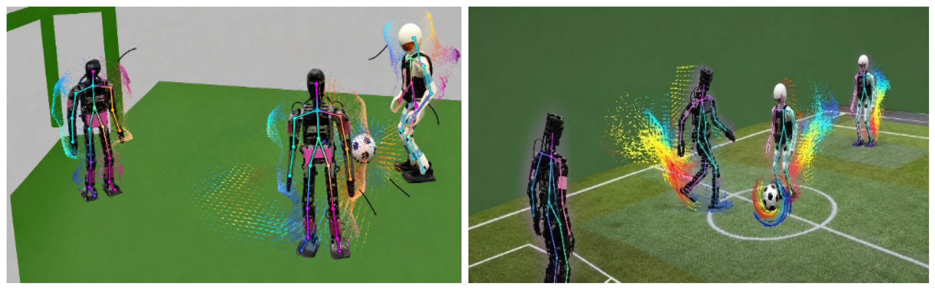
Figure 12.
Joint pose-flow feature extraction capturing spatial and temporal dynamics of humanoid robots.
Figure 12.
Joint pose-flow feature extraction capturing spatial and temporal dynamics of humanoid robots.
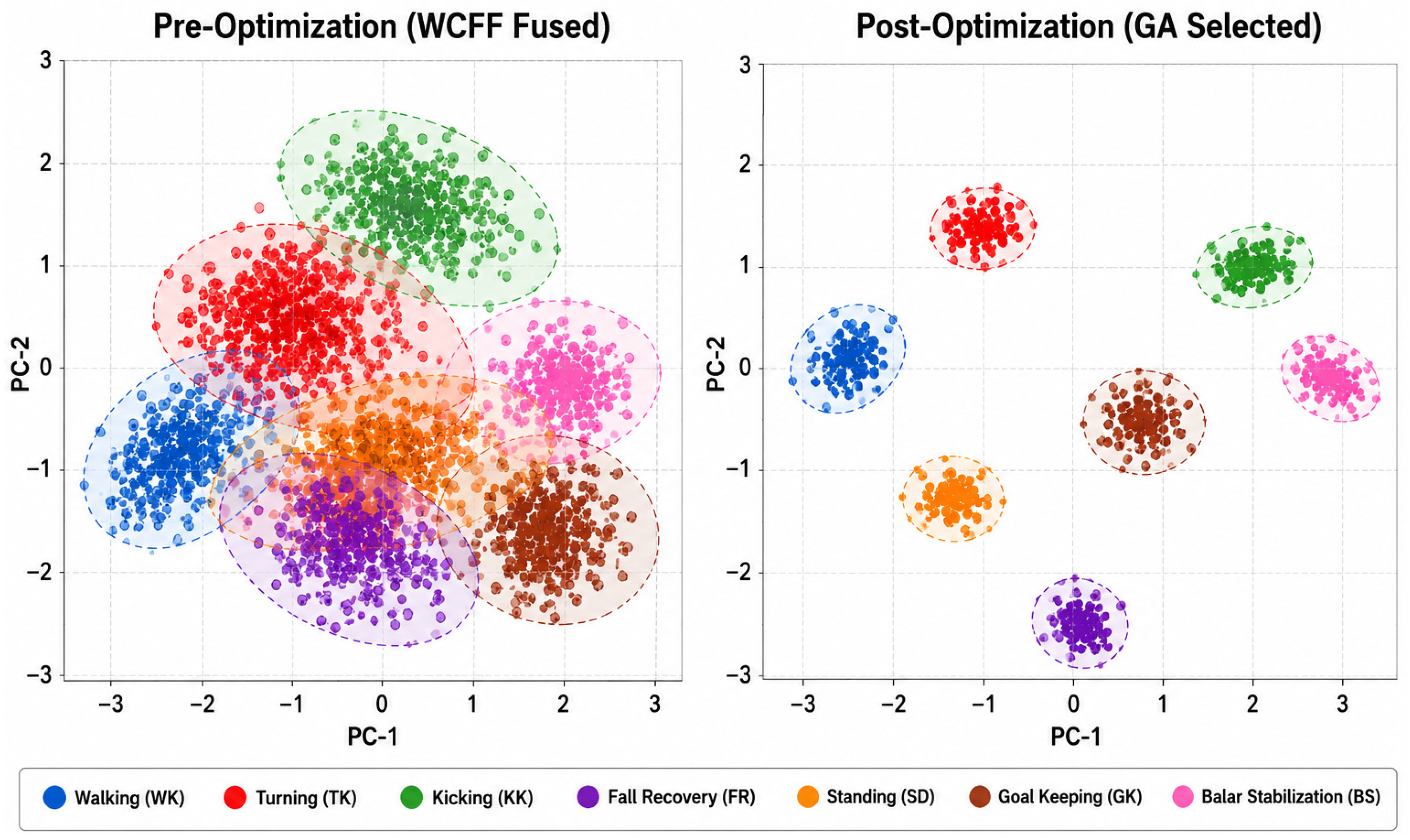
Figure 13.
Two-dimensional visualization of the multimodal feature space before and after GA-based feature optimization, showing improved class compactness and inter-class separation following the removal of redundant features.
Figure 13.
Two-dimensional visualization of the multimodal feature space before and after GA-based feature optimization, showing improved class compactness and inter-class separation following the removal of redundant features.
Figure 14.
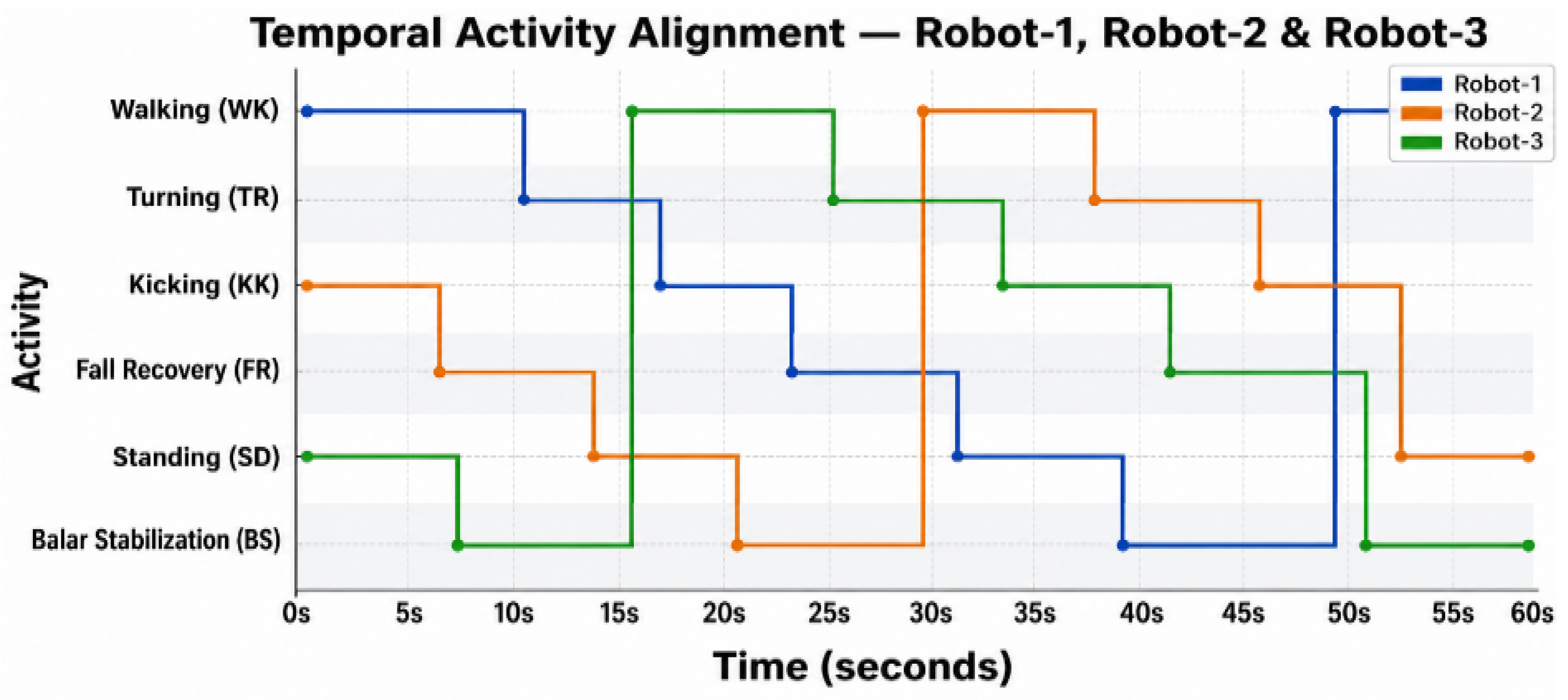
Temporal activity alignment and behavioral state transitions for Robot-1, Robot-2, and Robot-3 over a 60 s duration.
Figure 14.
Temporal activity alignment and behavioral state transitions for Robot-1, Robot-2, and Robot-3 over a 60 s duration.
Figure 15.
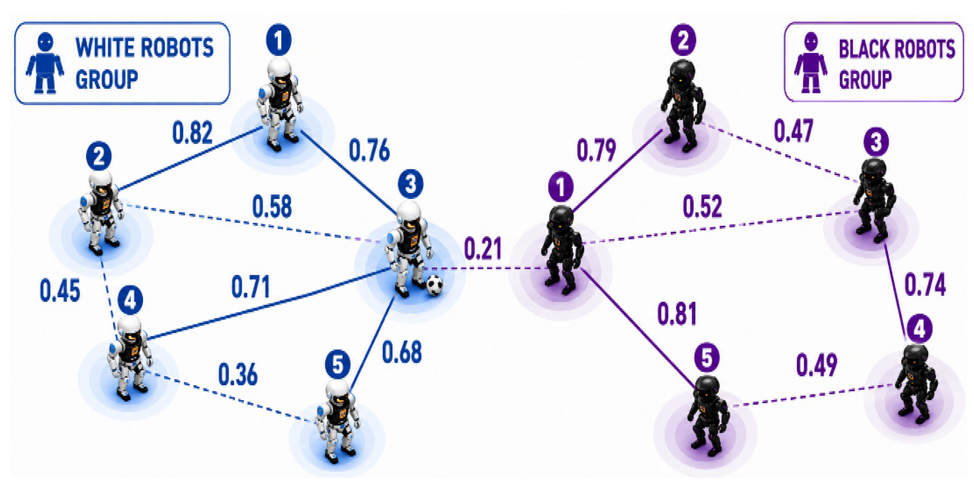
Interaction graph between the White Robots Group and Black Robots Group. Blue and purple colors denote the two robot groups, respectively; solid and dashed lines represent strong and weak interaction links, while the numbers on the edges indicate the corresponding interaction weights.
Figure 15.
Interaction graph between the White Robots Group and Black Robots Group. Blue and purple colors denote the two robot groups, respectively; solid and dashed lines represent strong and weak interaction links, while the numbers on the edges indicate the corresponding interaction weights.
Figure 16.
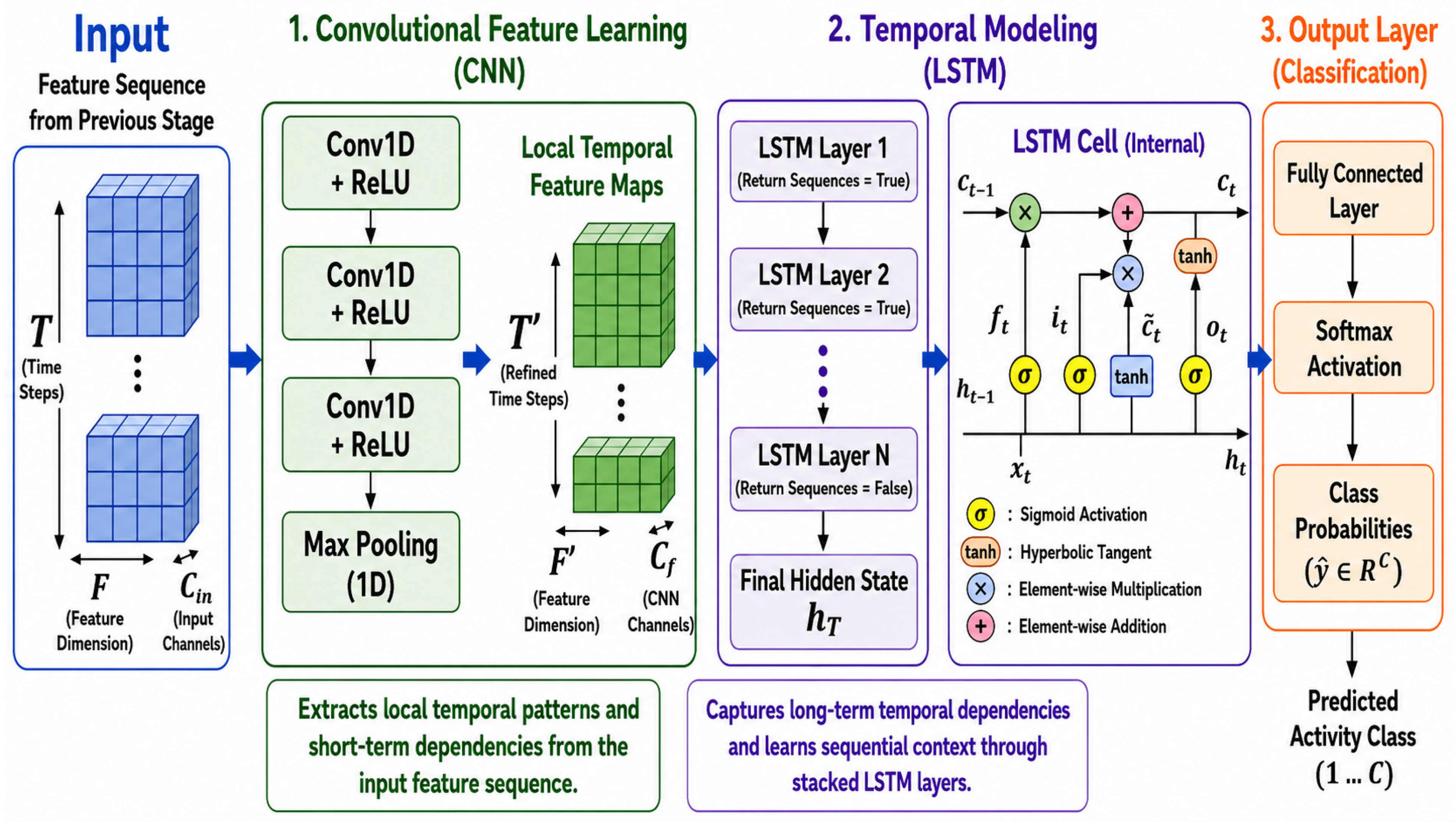
Proposed CNN–LSTM architecture for temporal feature learning and activity classification. Arrows indicate the data flow between processing stages, while colors distinguish the input, CNN feature extraction, LSTM temporal modeling, and output classification modules.
Figure 16.
Proposed CNN–LSTM architecture for temporal feature learning and activity classification. Arrows indicate the data flow between processing stages, while colors distinguish the input, CNN feature extraction, LSTM temporal modeling, and output classification modules.
Figure 17.
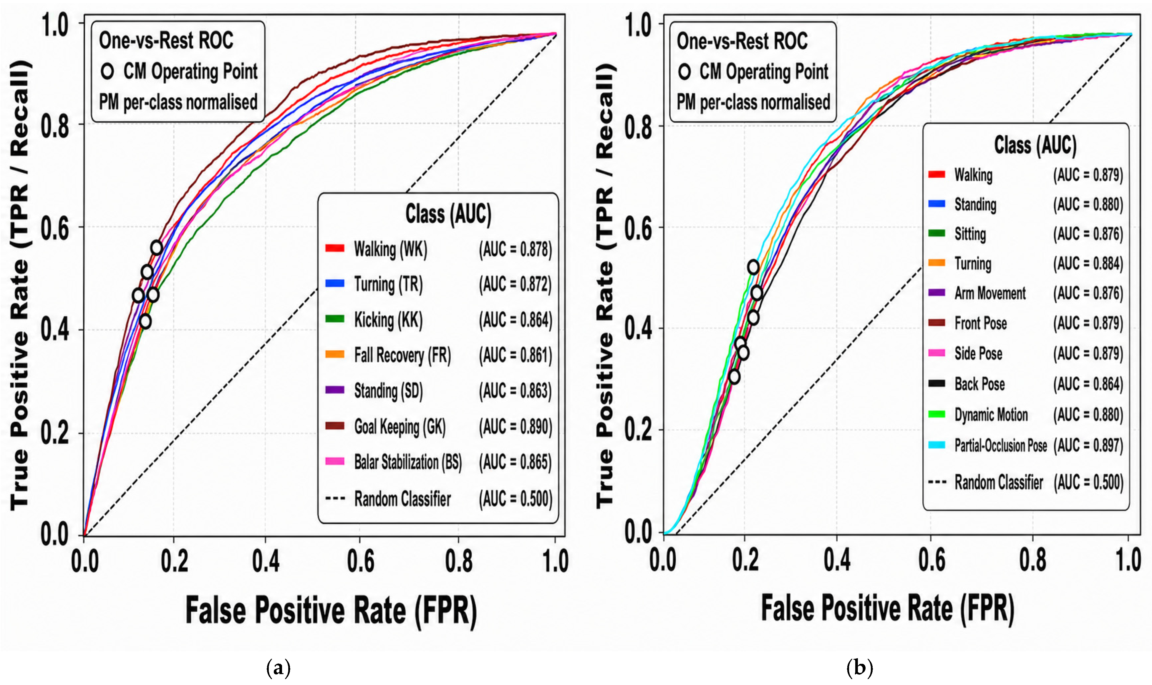
(a) Per-class ROC curves on the SoccerDiffusion (one-vs-rest); (b) HumanoidRobotPose dataset.
Figure 17.
(a) Per-class ROC curves on the SoccerDiffusion (one-vs-rest); (b) HumanoidRobotPose dataset.
Table 1.
Confusion matrix for the SoccerDiffusion dataset (per-class recognition rates, %).
Table 1.
Confusion matrix for the SoccerDiffusion dataset (per-class recognition rates, %).
| Actual/Predicted | WK | TR | KK | FR | SD | GK | BS |
|---|
| Walking (WK) | 85 | 4 | 5 | 2 | 1 | 2 | 1 |
| Turning (TR) | 5 | 84 | 3 | 3 | 2 | 2 | 1 |
| Kicking (KK) | 5 | 4 | 83 | 3 | 2 | 2 | 1 |
| Fall Recovery (FR) | 2 | 3 | 3 | 86 | 3 | 2 | 1 |
| Standing (SD) | 2 | 2 | 3 | 3 | 87 | 2 | 1 |
| Goal Keeping (GK) | 2 | 2 | 1 | 2 | 2 | 88 | 3 |
| Balar Stabilization (BS) | 1 | 1 | 1 | 1 | 1 | 2 | 93 |
Table 2.
Confusion matrix for the HumanoidRobotPose dataset (per-class recognition rates, %).
Table 2.
Confusion matrix for the HumanoidRobotPose dataset (per-class recognition rates, %).
| Actual/Predicted | Wlk | Std | Sit | Trn | ArM | FrP | SdP | BkP | DyM | POP |
|---|
| Walking (Wlk) | 87 | 2 | 1 | 3 | 2 | 1 | 1 | 1 | 1 | 1 |
| Standing (Std) | 2 | 86 | 3 | 1 | 2 | 2 | 1 | 1 | 1 | 1 |
| Sitting (Sit) | 1 | 3 | 87 | 1 | 2 | 2 | 1 | 1 | 1 | 1 |
| Turning (Trn) | 3 | 1 | 1 | 88 | 2 | 1 | 1 | 1 | 1 | 1 |
| Arm Movement (ArM) | 1 | 2 | 1 | 1 | 89 | 2 | 1 | 1 | 1 | 1 |
| Front Pose (FrP) | 1 | 2 | 1 | 1 | 2 | 87 | 2 | 2 | 1 | 1 |
| Side Pose (SdP) | 1 | 1 | 1 | 1 | 2 | 2 | 88 | 2 | 1 | 1 |
| Back Pose (BkP) | 1 | 1 | 1 | 1 | 2 | 2 | 2 | 86 | 2 | 2 |
| Dynamic Motion (DyM) | 1 | 1 | 1 | 1 | 2 | 1 | 1 | 2 | 89 | 1 |
| Partial-Occlusion (POP) | 1 | 1 | 1 | 1 | 1 | 1 | 1 | 1 | 1 | 91 |
Table 3.
Precision, recall, and F1-score on the SoccerDiffusion dataset.
Table 3.
Precision, recall, and F1-score on the SoccerDiffusion dataset.
| Class | Precision (%) | Recall (%) | F1-Score (%) |
|---|
| Walking (WK) | 83.33 | 85.00 | 84.16 |
| Turning (TR) | 84.00 | 84.00 | 84.00 |
| Kicking (KK) | 83.84 | 83.00 | 83.42 |
| Fall Recovery (FR) | 86.00 | 86.00 | 86.00 |
| Standing (SD) | 88.78 | 87.00 | 87.88 |
| Goal Keeping (GK) | 88.00 | 88.00 | 88.00 |
| Balar Stabilization (BS) | 92.08 | 93.00 | 92.54 |
| Macro Average | 86.58 | 86.57 | 86.57 |
Table 4.
Precision, recall, and F1-score on the HumanoidRobotPose dataset.
Table 4.
Precision, recall, and F1-score on the HumanoidRobotPose dataset.
| Class | Precision (%) | Recall (%) | F1-Score (%) |
|---|
| Walking | 87.00 | 87.00 | 87.00 |
| Standing | 86.00 | 86.00 | 86.00 |
| Sitting | 87.87 | 87.00 | 87.43 |
| Turning | 88.88 | 88.00 | 88.43 |
| Arm Movement | 85.57 | 89.00 | 87.25 |
| Front Pose | 86.13 | 87.00 | 86.56 |
| Side Pose | 88.00 | 88.00 | 88.00 |
| Back Pose | 87.75 | 86.00 | 86.86 |
| Dynamic Motion | 89.89 | 89.00 | 89.44 |
| Partial-Occlusion Pose | 91.00 | 91.00 | 91.00 |
| Macro Average | 87.81 | 87.80 | 87.80 |
Table 5.
Five-fold subject-independent cross-validation results of the proposed multimodal framework on the SoccerDiffusion and HumanoidRobotPose datasets (mean ± standard deviation).
Table 5.
Five-fold subject-independent cross-validation results of the proposed multimodal framework on the SoccerDiffusion and HumanoidRobotPose datasets (mean ± standard deviation).
| Fold | SoccerDiffusion Acc. | SoccerDiffusion Macro-F1 | HumanoidRobotPose Acc. | HumanoidRobotPose Macro-F1 |
|---|
| Fold 1 | 85.92 | 85.55 | 87.43 | 87.12 |
| Fold 2 | 86.48 | 86.10 | 88.11 | 87.81 |
| Fold 3 | 87.08 | 86.73 | 88.63 | 88.36 |
| Fold 4 | 86.77 | 86.38 | 88.29 | 88.01 |
| Fold 5 | 86.55 | 86.18 | 87.74 | 87.46 |
| Mean ± SD | 86.56 ± 0.44 | 86.19 ± 0.42 | 88.04 ± 0.46 | 87.75 ± 0.47 |
Table 6.
Robustness analysis of the proposed framework under different random seed initializations, demonstrating the stability and reproducibility of the reported recognition performance.
Table 6.
Robustness analysis of the proposed framework under different random seed initializations, demonstrating the stability and reproducibility of the reported recognition performance.
| Seed | SoccerDiffusion | HumanoidRobotPose |
|---|
| 42 | 86.56 | 88.04 |
| 7 | 86.14 | 87.69 |
| 123 | 86.83 | 88.31 |
| 2024 | 86.37 | 87.91 |
| 31,337 | 86.91 | 88.22 |
| Mean ± SD | 86.56 ± 0.31 | 88.03 ± 0.25 |
Table 7.
Leakage prevention strategy adopted throughout the experimental pipeline.
Table 7.
Leakage prevention strategy adopted throughout the experimental pipeline.
| Pipeline Stage | Training Data Only | Test Data Used During Fitting | Leakage Risk | Mitigation Strategy |
|---|
| Subject-independent split | ✓ | No | None | Dataset partitioned before any learnable operation. |
| KELM preprocessing | ✓ | No | Low | KELM parameters estimated exclusively from the training partition and applied unchanged to the test set. |
| KCCF kernel learning | ✓ | No | Low | Kernel mappings are learned only from training samples. |
| Entropy-monitoring windowing | N/A | No | None | Applied independently to each signal without dataset-level statistics. |
| MINIROCKET/TS-CHIEF/r-STSF | ✓ | No | Low | Feature extraction fitted only on training data. |
| WCFF fusion | ✓ | No | Low | Fusion weights are estimated exclusively using training features. |
| Genetic Algorithm | ✓ | No | Medium | Feature selection optimized only on the training partition. |
| GPSM | ✓ | No | Low | Model trained exclusively on training sequences. |
| DeepConvLSTM | ✓ | No | None | Network optimized only using the training partition. |
Table 8.
Performance comparison with representative unimodal and multimodal state-of-the-art methods.
Table 8.
Performance comparison with representative unimodal and multimodal state-of-the-art methods.
| Method | Modality | Soccer Diffusion Acc. (%) | HumanoidRobotPose Acc. (%) |
|---|
| DeepConvLSTM [35] | IMU | 79.43 | 81.22 |
| Transformer-based diffusion model [36] | IMU | 81.05 | 82.87 |
| TimeSformer [20] | RGB (Vision Transformer) | 82.18 | 83.76 |
| VideoMAE V2 [32] | RGB (Masked Video Transformer) | 83.54 | 85.08 |
| HAMLET [37] | IMU + RGB | 82.60 | 83.94 |
| BodyFormer [38] | IMU + Skeleton | 83.78 | 85.31 |
| HARFusion [39] | IMU + RGB | 84.12 | 86.09 |
| HRNet [40] | IMU + Video | 84.97 | 86.73 |
| Proposed Method | IMU + RGB | 86.56 | 88.04 |
Table 9.
Fusion ablation with the classifier held constant.
Table 9.
Fusion ablation with the classifier held constant.
| Configuration | Classifier | Soccer Diffusion Acc. (%) | HumanoidRobotPose Acc. (%) |
|---|
| (1) IMU branch only | DeepConvLSTM | 81.20 | 83.05 |
| (2) RGB branch only | DeepConvLSTM | 82.67 | 84.10 |
| (3) Naïve concatenation | DeepConvLSTM | 83.75 | 85.20 |
| (4) WCFF fusion, without GA | DeepConvLSTM | 84.89 | 86.15 |
| (5) WCFF + GA (proposed) | DeepConvLSTM | 86.56 | 88.04 |
Table 10.
Computational complexity (Big-O) and per-segment wall-clock time of each pipeline stage.
Table 10.
Computational complexity (Big-O) and per-segment wall-clock time of each pipeline stage.
| Stage | Time Complexity | Space Complexity | Per-Segment Time (ms) |
|---|
| KELM Preprocessing | O(T3) | O(T2) | 8.4 |
| KCCF Multikernel Fusion | O(M T3) | O(M T2) | 21.3 |
| Entropy-Monitoring Windowing | O(T B) | O(B) | 1.2 |
| MINIROCKET | O(N T) | O(N) | 3.6 |
| TS-CHIEF | O(Kt T log T) | O(Kt T) | 12.5 |
| r-STSF | O(Kr T log T) | O(Kr T) | 9.8 |
| Anisotropic Diffusion | O(n H W) | O(H W) | 5.7 |
| HRNet Silhouette | O(H W C) | O(H W C) | 18.2 |
| DensePose R-CNN | O(H W C) | O(H W C) | 26.8 |
| Mesh Graphormer | O(|V|2 d) | O(|V| d) | 22.4 |
| MPFF | O(J T) | O(J T) | 4.1 |
| WCFF | O(D3) | O(D2) | 11.5 |
| Genetic Algorithm | O(G P D) | O(P D) | 14.7 |
| Cluster-based Sequence Alignment | O(K T) | O(K T) | 6.2 |
| Gaussian Process Sequence Model | O(T3) | O(T2) | 9.1 |
| DeepConvLSTM | O(T D h + T h2) | O(T h) | 23.6 |




 ,
,