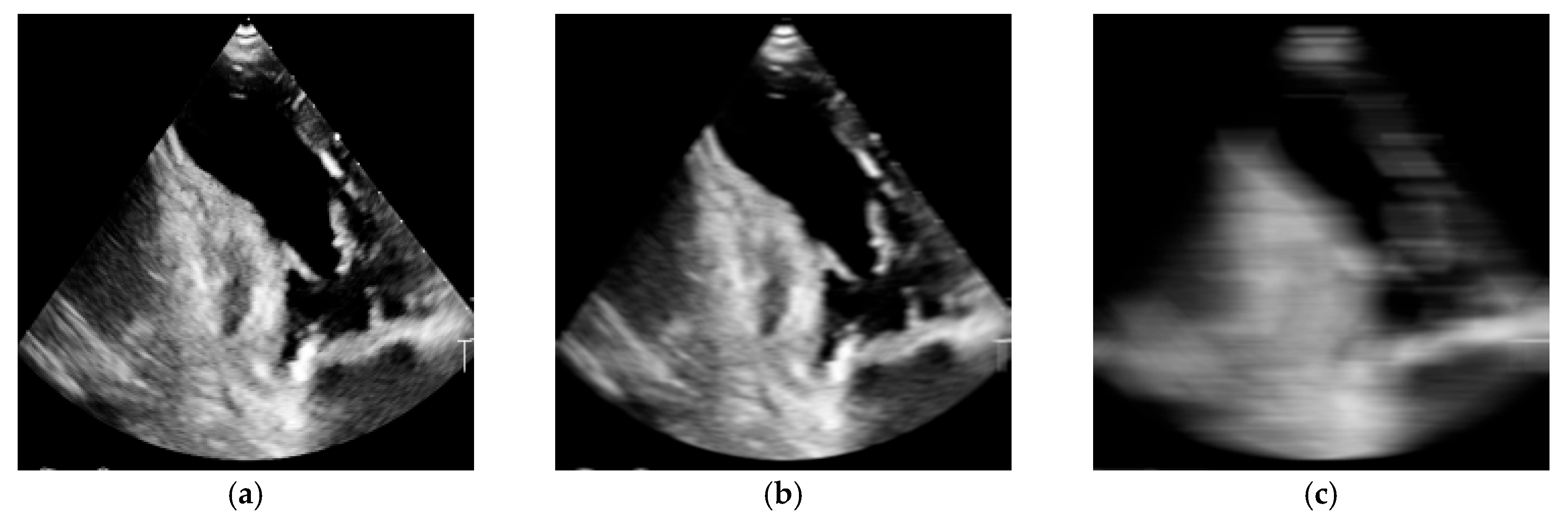
Figure 1.
Example of simulated motion blur artifact in a transthoracic echocardiographic image. From left: (a) reference image without distortion (kernel size = 0), (b) image with mild blurring (kernel size = 5), (c) image with severe blurring (kernel size = 20).
Figure 1.
Example of simulated motion blur artifact in a transthoracic echocardiographic image. From left: (a) reference image without distortion (kernel size = 0), (b) image with mild blurring (kernel size = 5), (c) image with severe blurring (kernel size = 20).
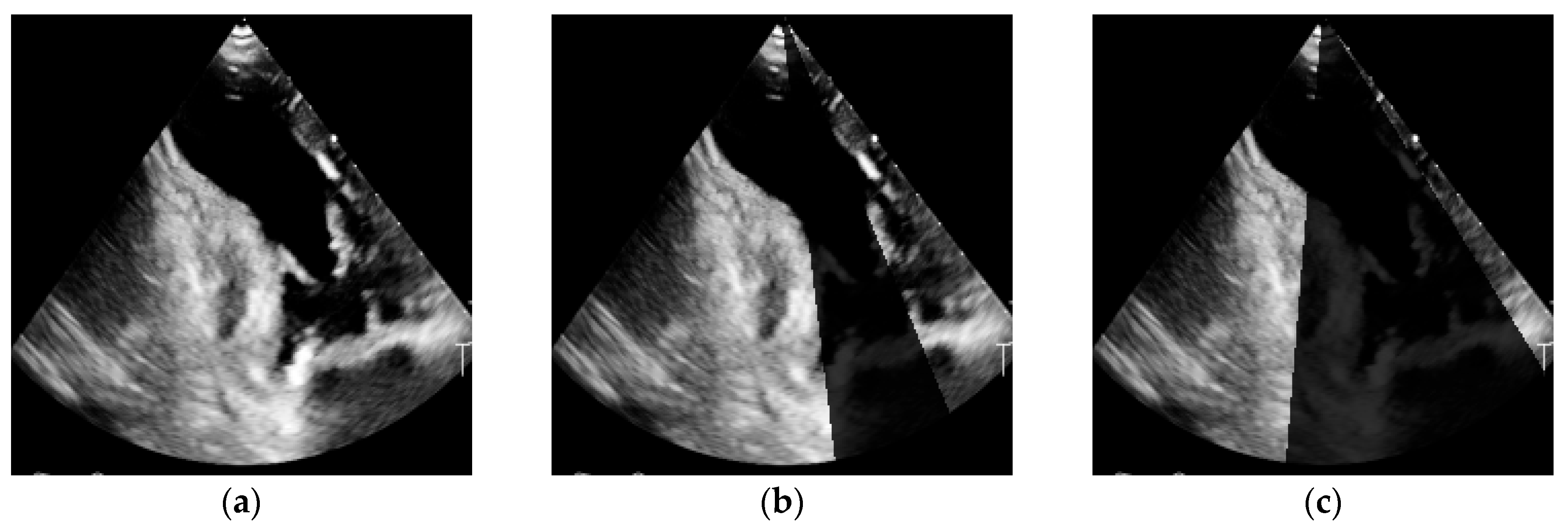
Figure 2.
Example of simulated acoustic shadowing artifact in a transthoracic echocardiographic image. From left: (a) reference image without distortion (shadow width = 0), (b) image with a narrow shadow (shadow width = 0.3), and (c) image with a wide shadow (shadow width = 0.7).
Figure 2.
Example of simulated acoustic shadowing artifact in a transthoracic echocardiographic image. From left: (a) reference image without distortion (shadow width = 0), (b) image with a narrow shadow (shadow width = 0.3), and (c) image with a wide shadow (shadow width = 0.7).
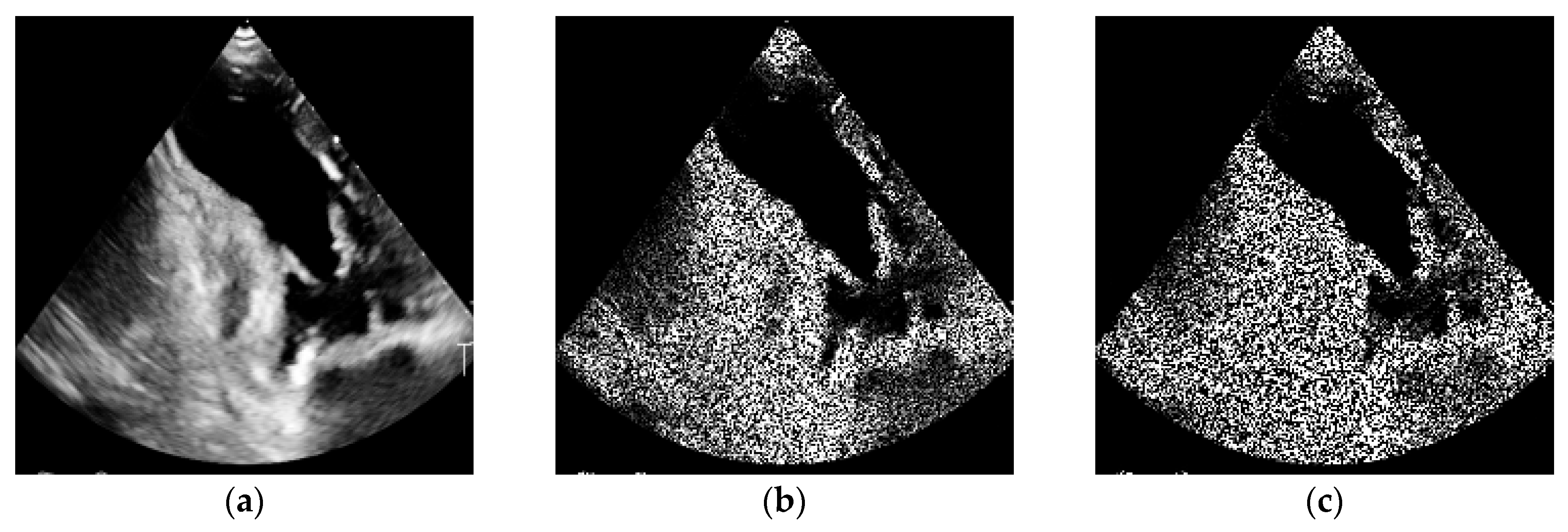
Figure 3.
Example of simulated speckle noise artifact in a transthoracic echocardiographic image. From left: (a) reference image without distortion (noise amount = 0), (b) image with a moderate noise level (noise amount = 1), (c) image with a high noise level (noise amount = 3). With increasing values of the noise amount parameter, the granular speckle pattern becomes more pronounced, hindering the interpretation of the echocardiogram.
Figure 3.
Example of simulated speckle noise artifact in a transthoracic echocardiographic image. From left: (a) reference image without distortion (noise amount = 0), (b) image with a moderate noise level (noise amount = 1), (c) image with a high noise level (noise amount = 3). With increasing values of the noise amount parameter, the granular speckle pattern becomes more pronounced, hindering the interpretation of the echocardiogram.
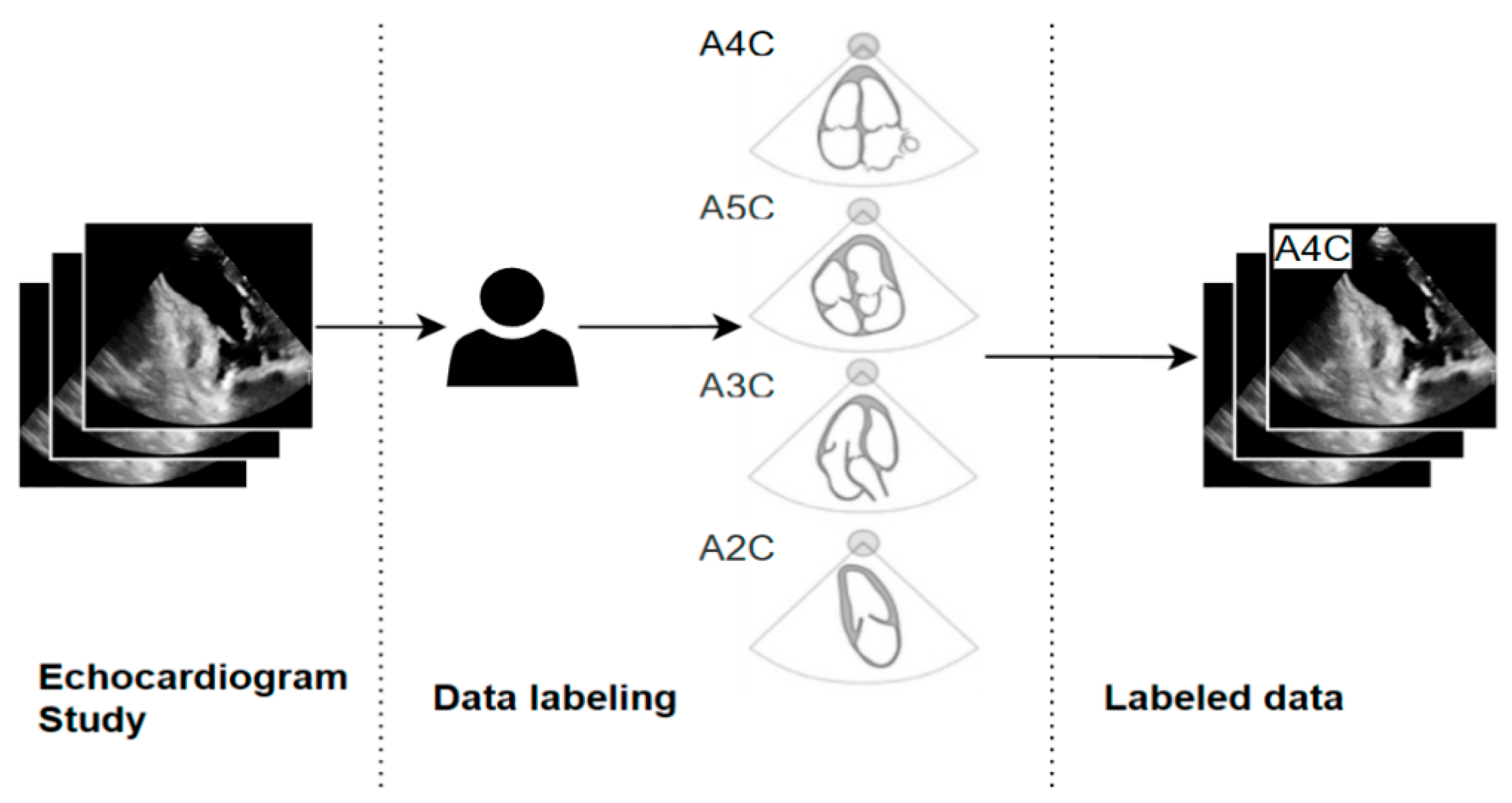
Figure 4.
Schematic representation of the echocardiographic data labeling process. Raw TTE images were manually annotated by an expert and assigned to the corresponding cardiac views (A2C, A3C, A4C, A5C). The resulting labeled dataset constituted the basis for subsequent preprocessing and training of CNN models. (TTE—transthoracic echocardiography; A2C—apical two-chamber; A3C—apical three-chamber; A4C—apical four-chamber; A5C—apical five-chamber).
Figure 4.
Schematic representation of the echocardiographic data labeling process. Raw TTE images were manually annotated by an expert and assigned to the corresponding cardiac views (A2C, A3C, A4C, A5C). The resulting labeled dataset constituted the basis for subsequent preprocessing and training of CNN models. (TTE—transthoracic echocardiography; A2C—apical two-chamber; A3C—apical three-chamber; A4C—apical four-chamber; A5C—apical five-chamber).
Figure 5.
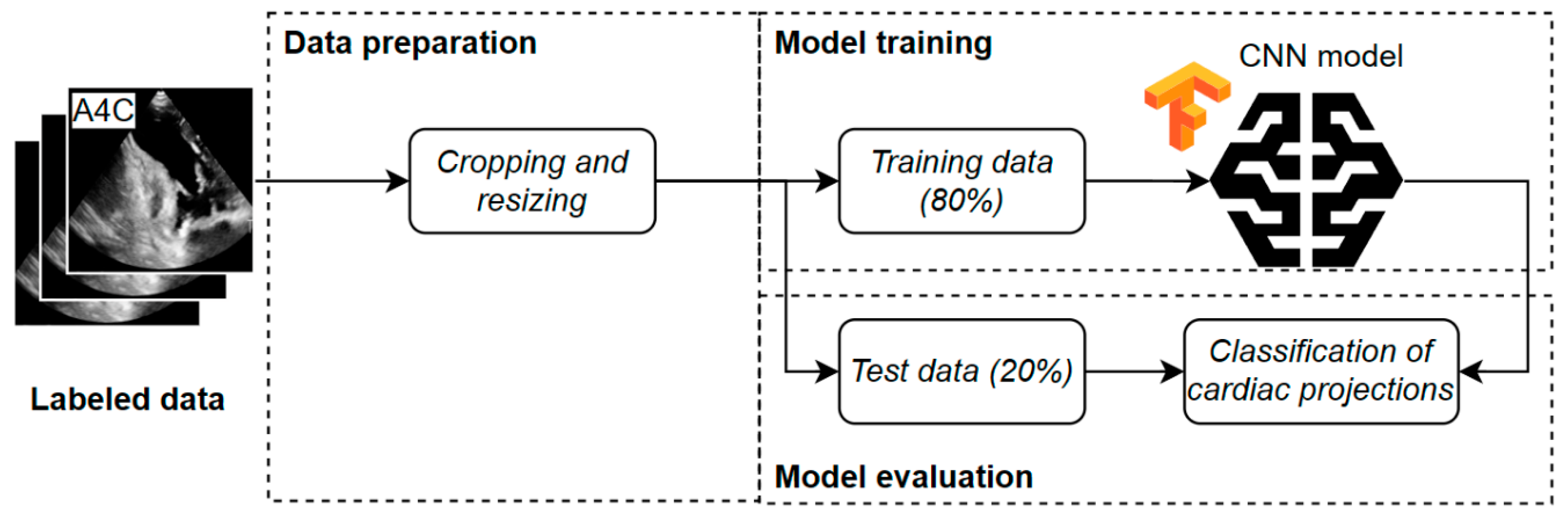
General workflow of the experiment. The labeled data were subjected to preprocessing (cropping and resizing) and subsequently divided into training and test sets. CNN models (ResNet-18, ResNet-34) were then trained to classify cardiac views. (CNN—convolutional neural network).
Figure 5.
General workflow of the experiment. The labeled data were subjected to preprocessing (cropping and resizing) and subsequently divided into training and test sets. CNN models (ResNet-18, ResNet-34) were then trained to classify cardiac views. (CNN—convolutional neural network).
Figure 6.
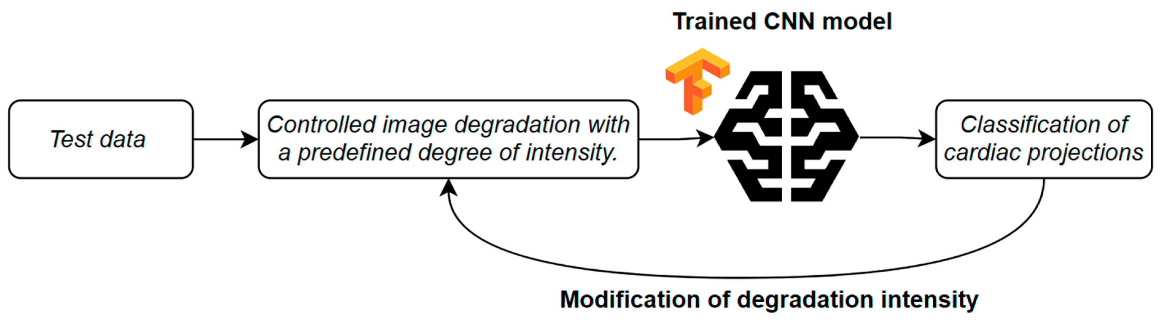
Schematic representation of the procedure for assessing CNN robustness to image degradation. Test data were subjected to controlled degradation with a defined intensity level and subsequently classified using the trained model. The process was repeated across varying degradation intensities to analyze the impact of artifacts on the classification performance of echocardiographic views. (CNN—convolutional neural network).
Figure 6.
Schematic representation of the procedure for assessing CNN robustness to image degradation. Test data were subjected to controlled degradation with a defined intensity level and subsequently classified using the trained model. The process was repeated across varying degradation intensities to analyze the impact of artifacts on the classification performance of echocardiographic views. (CNN—convolutional neural network).
Figure 7.
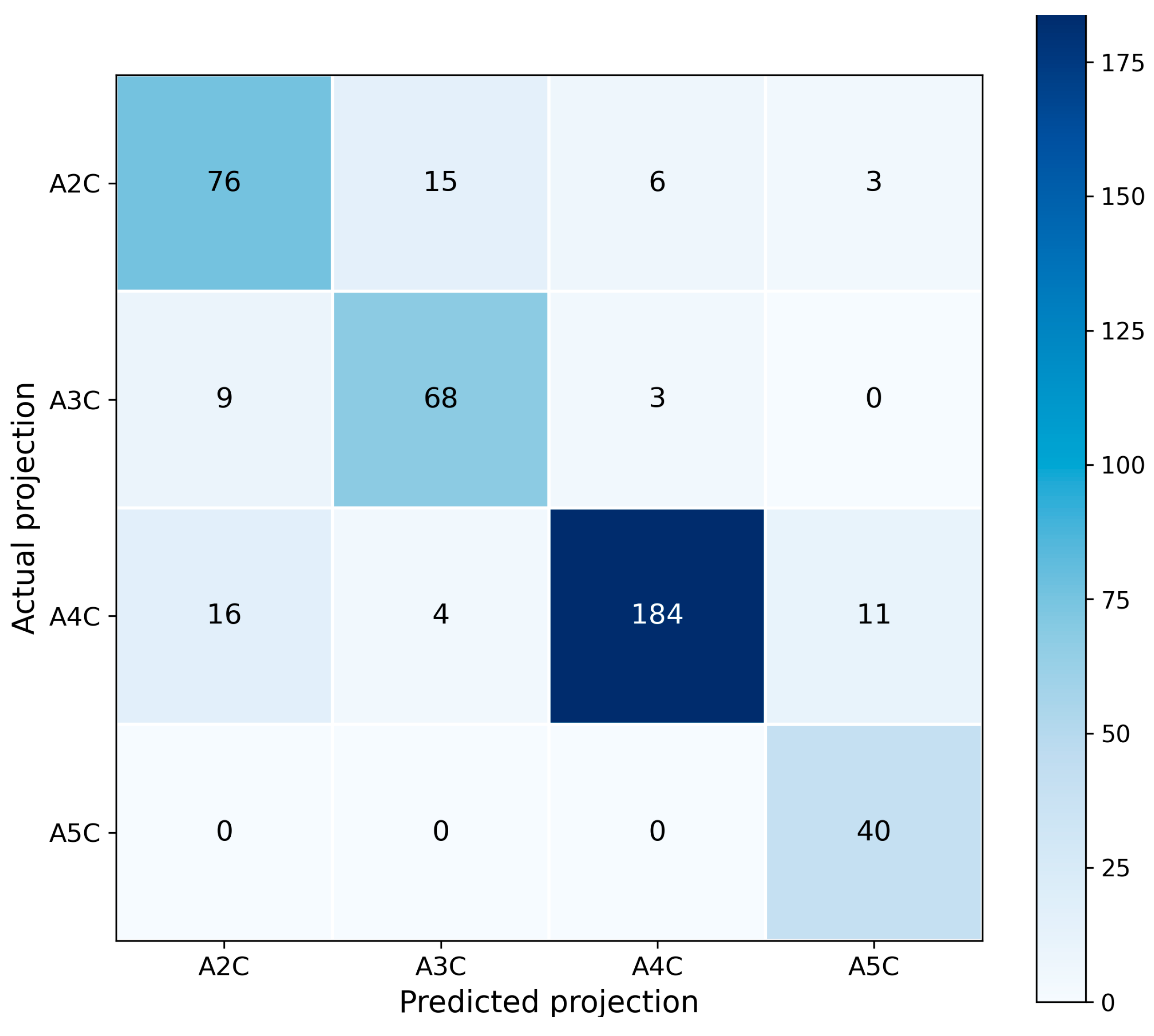
Frame-level confusion matrix for ResNet-18 on the independent test set.
Figure 7.
Frame-level confusion matrix for ResNet-18 on the independent test set.
Figure 8.
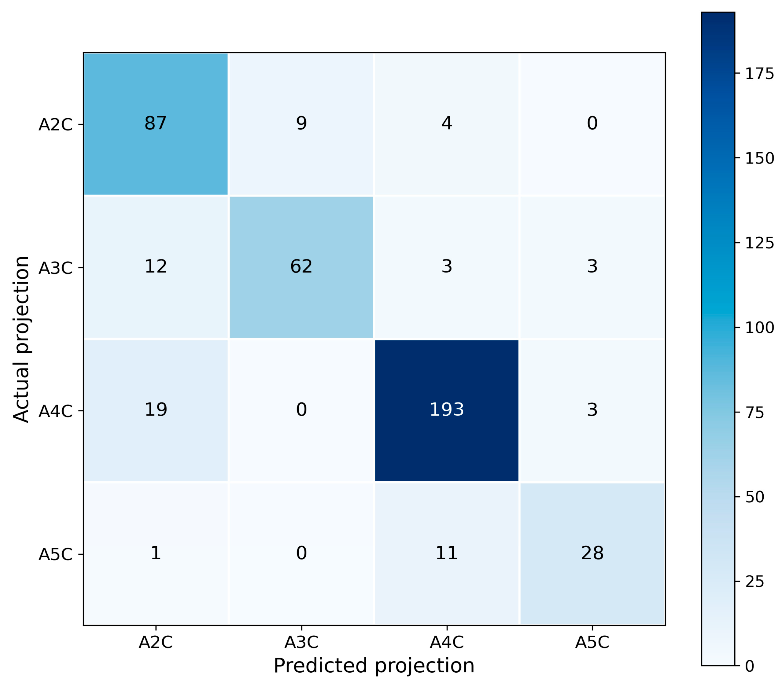
Frame-level confusion matrix for ResNet-34 on the independent test set.
Figure 8.
Frame-level confusion matrix for ResNet-34 on the independent test set.
Figure 9.
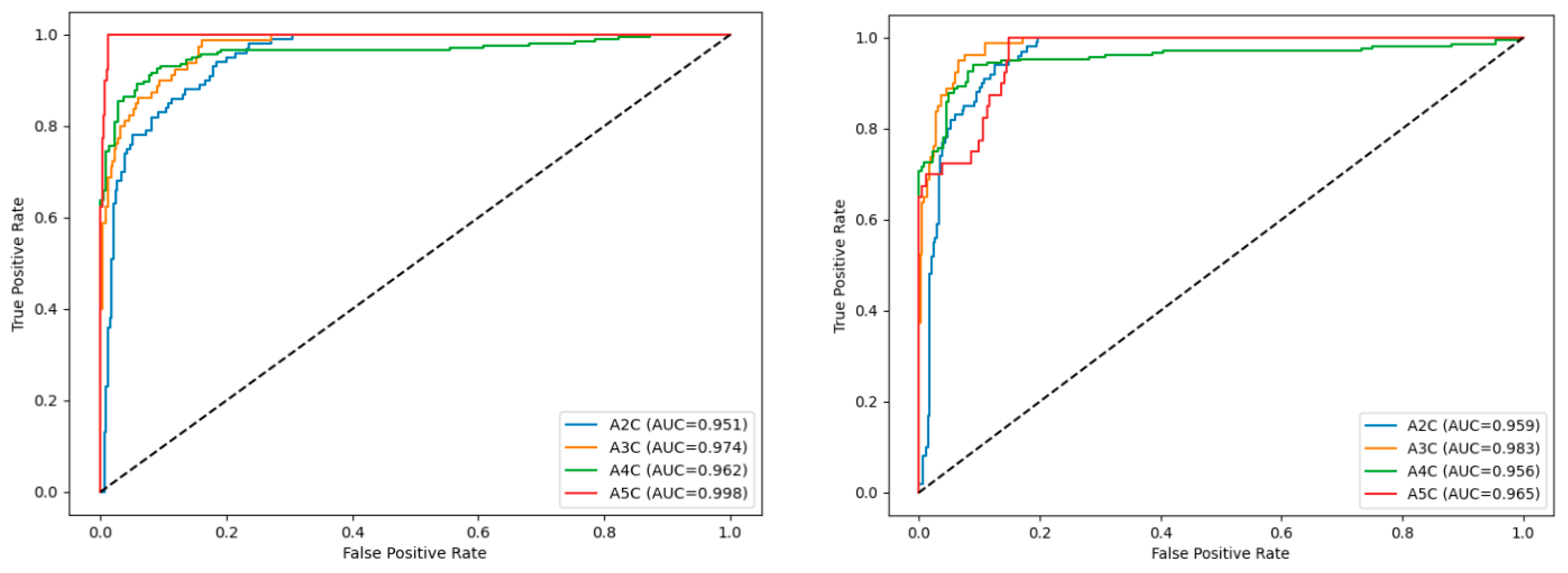
Receiver operating characteristic (ROC) curves for individual echocardiographic views obtained using the ResNet-18 model (left) and the ResNet-34 model (right). The area under the curve (AUC) values are reported separately for the A2C, A3C, A4C, and A5C classes. (A2C—apical two-chamber; A3C—apical three-chamber; A4C—apical four-chamber; A5C—apical five-chamber). The dashed diagonal line represents the performance of a random classifier, corresponding to an AUC of 0.5.
Figure 9.
Receiver operating characteristic (ROC) curves for individual echocardiographic views obtained using the ResNet-18 model (left) and the ResNet-34 model (right). The area under the curve (AUC) values are reported separately for the A2C, A3C, A4C, and A5C classes. (A2C—apical two-chamber; A3C—apical three-chamber; A4C—apical four-chamber; A5C—apical five-chamber). The dashed diagonal line represents the performance of a random classifier, corresponding to an AUC of 0.5.
Figure 10.
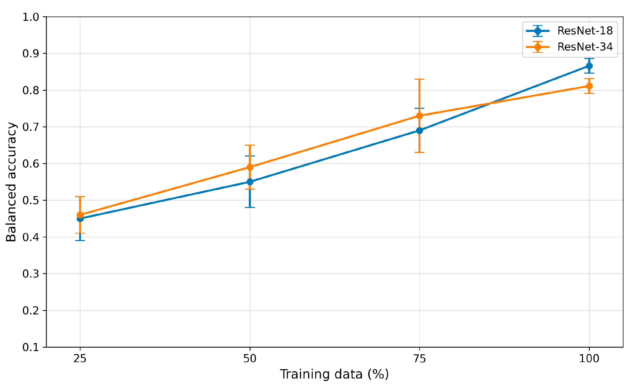
Learning curve showing the effect of training dataset size on balanced accuracy for ResNet-18 and ResNet-34 architectures.
Figure 10.
Learning curve showing the effect of training dataset size on balanced accuracy for ResNet-18 and ResNet-34 architectures.
Figure 11.
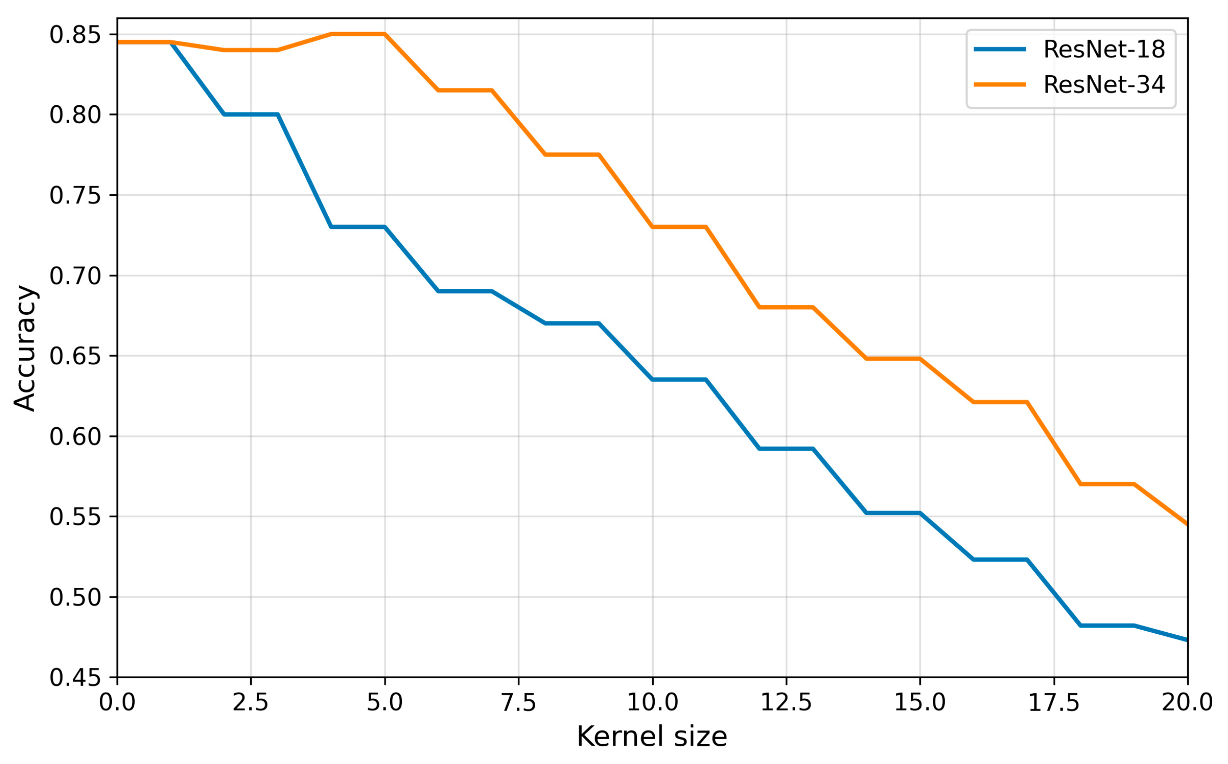
Classification accuracy as a function of motion blur kernel size for ResNet-18 and ResNet-34 models.
Figure 11.
Classification accuracy as a function of motion blur kernel size for ResNet-18 and ResNet-34 models.
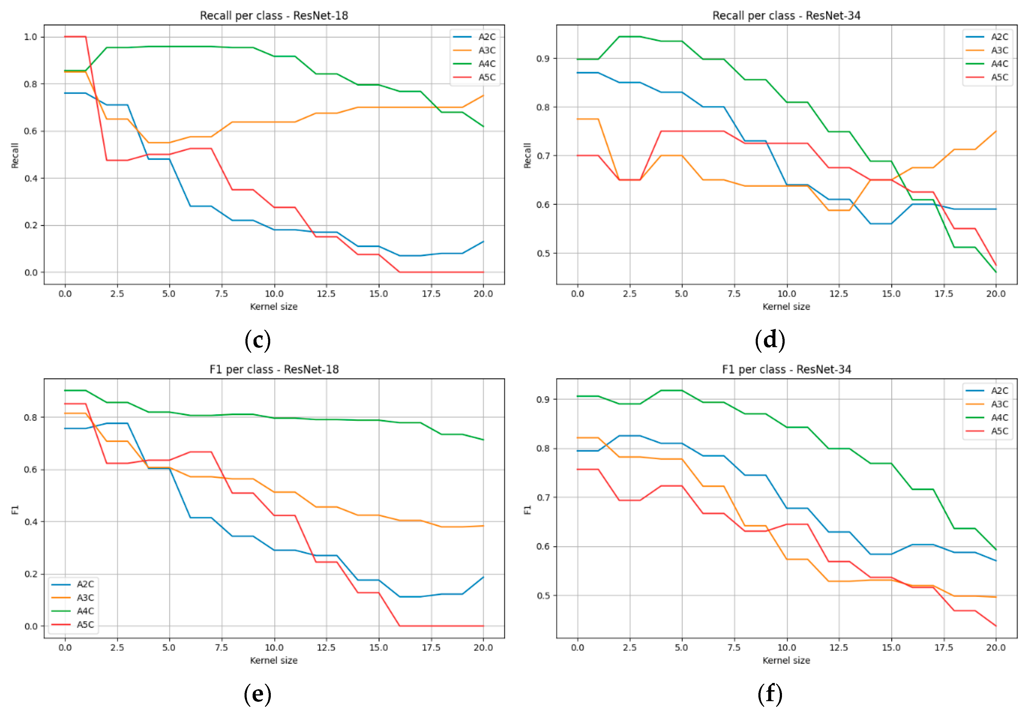
Figure 12.
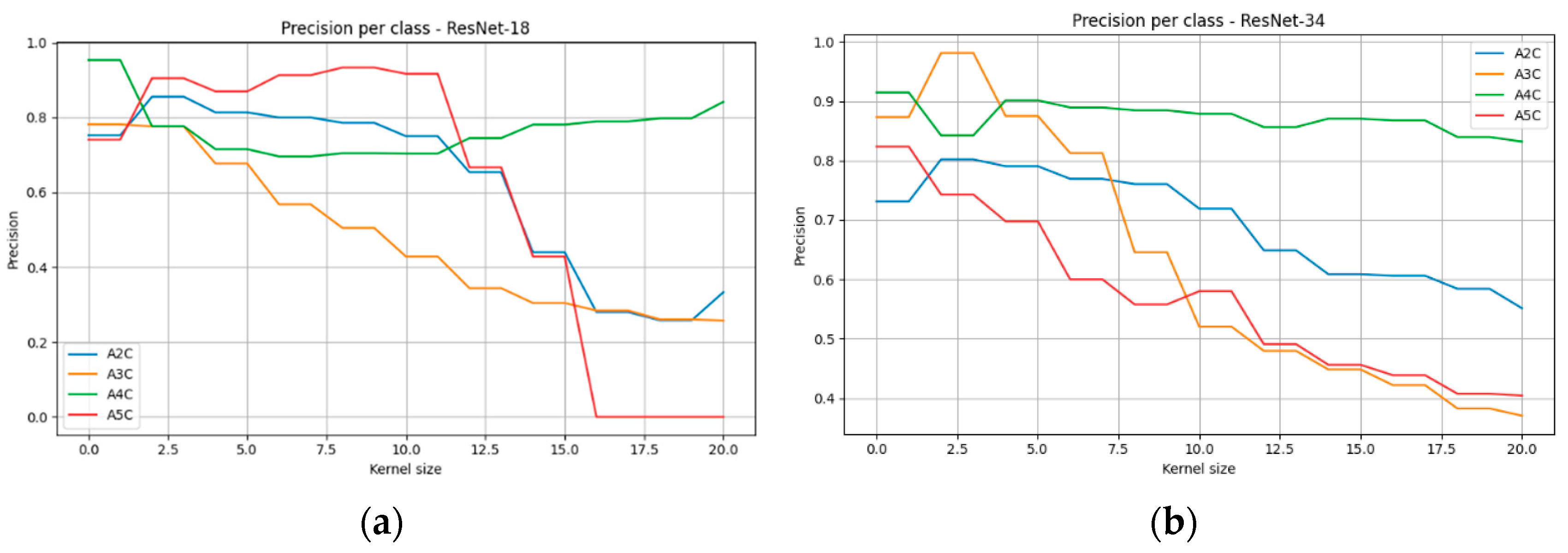
Impact of motion blur artifact on the classification performance of transthoracic echocardiographic views for ResNet-18 and ResNet-34 models. Results are presented separately for precision (a,b), recall (c,d), and F1-score (e,f).
Figure 12.
Impact of motion blur artifact on the classification performance of transthoracic echocardiographic views for ResNet-18 and ResNet-34 models. Results are presented separately for precision (a,b), recall (c,d), and F1-score (e,f).
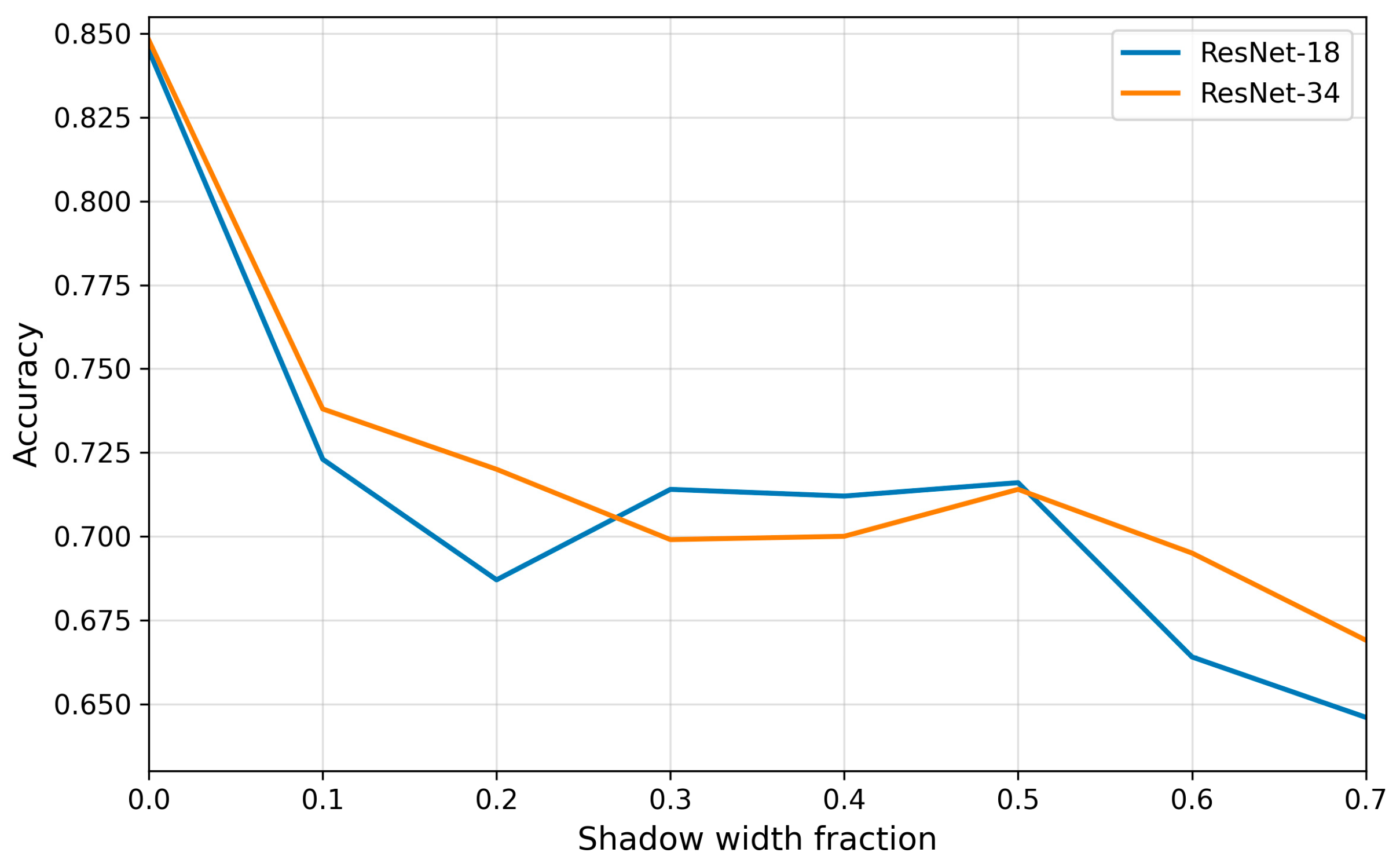
Figure 13.
Classification accuracy of transthoracic echocardiographic views as a function of acoustic shadow width for ResNet-18 and ResNet-34 models.
Figure 13.
Classification accuracy of transthoracic echocardiographic views as a function of acoustic shadow width for ResNet-18 and ResNet-34 models.
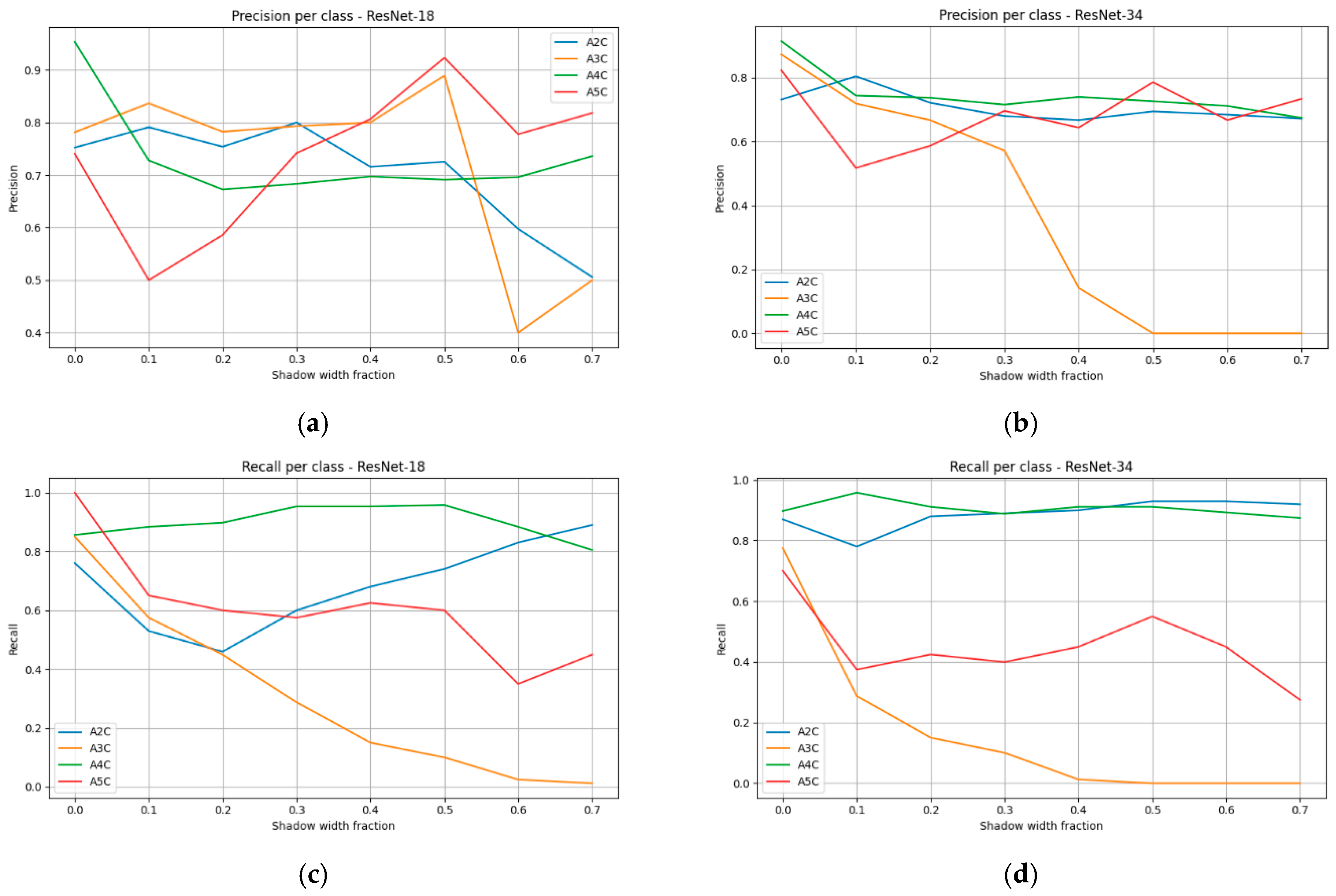
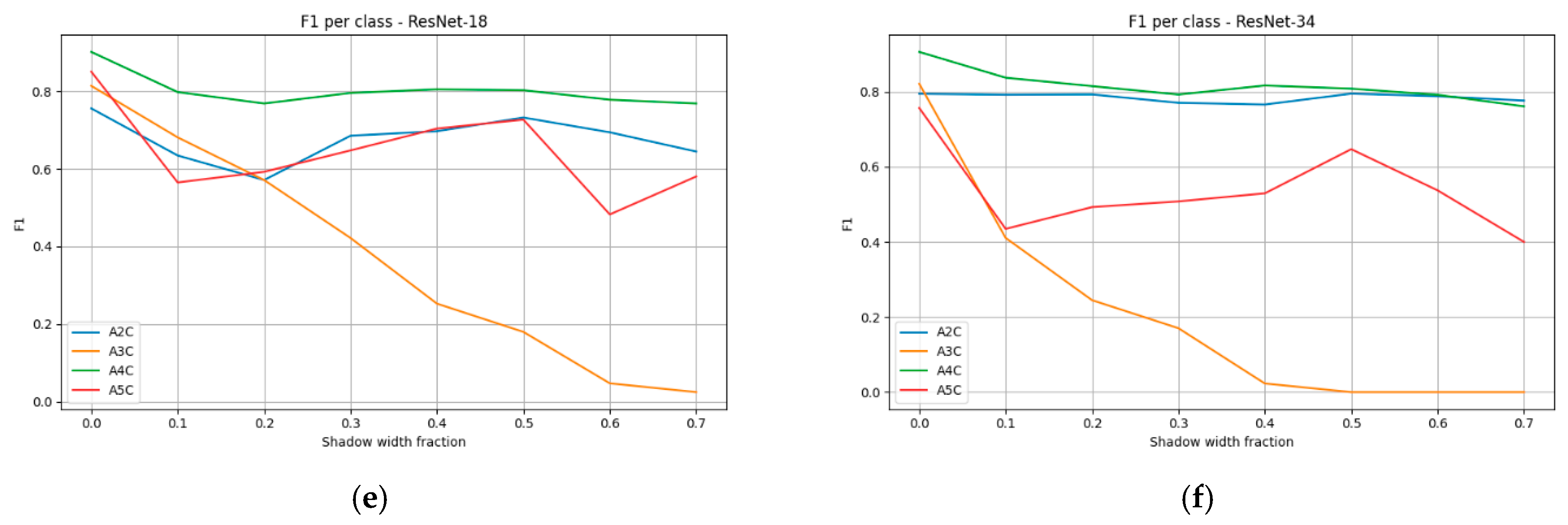
Figure 14.
Impact of acoustic shadow width on the classification performance of transthoracic echocardiographic views for ResNet-18 and ResNet-34 models. Results are presented separately for precision (a,b), recall (c,d), and F1-score (e,f), broken down by projection classes: A2C, A3C, A4C, and A5C.
Figure 14.
Impact of acoustic shadow width on the classification performance of transthoracic echocardiographic views for ResNet-18 and ResNet-34 models. Results are presented separately for precision (a,b), recall (c,d), and F1-score (e,f), broken down by projection classes: A2C, A3C, A4C, and A5C.
Figure 15.
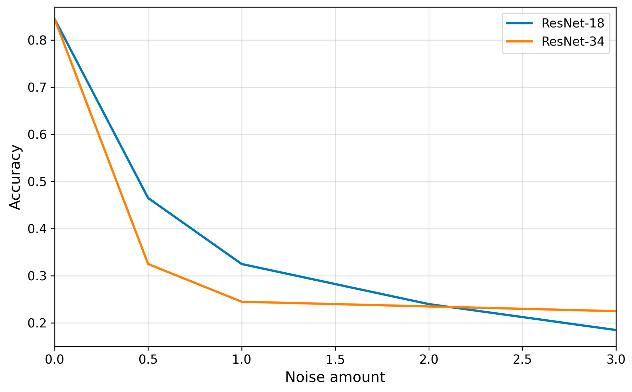
Classification accuracy as a function of speckle noise level (noise amount) for ResNet-18 and ResNet-34 models.
Figure 15.
Classification accuracy as a function of speckle noise level (noise amount) for ResNet-18 and ResNet-34 models.
Figure 16.
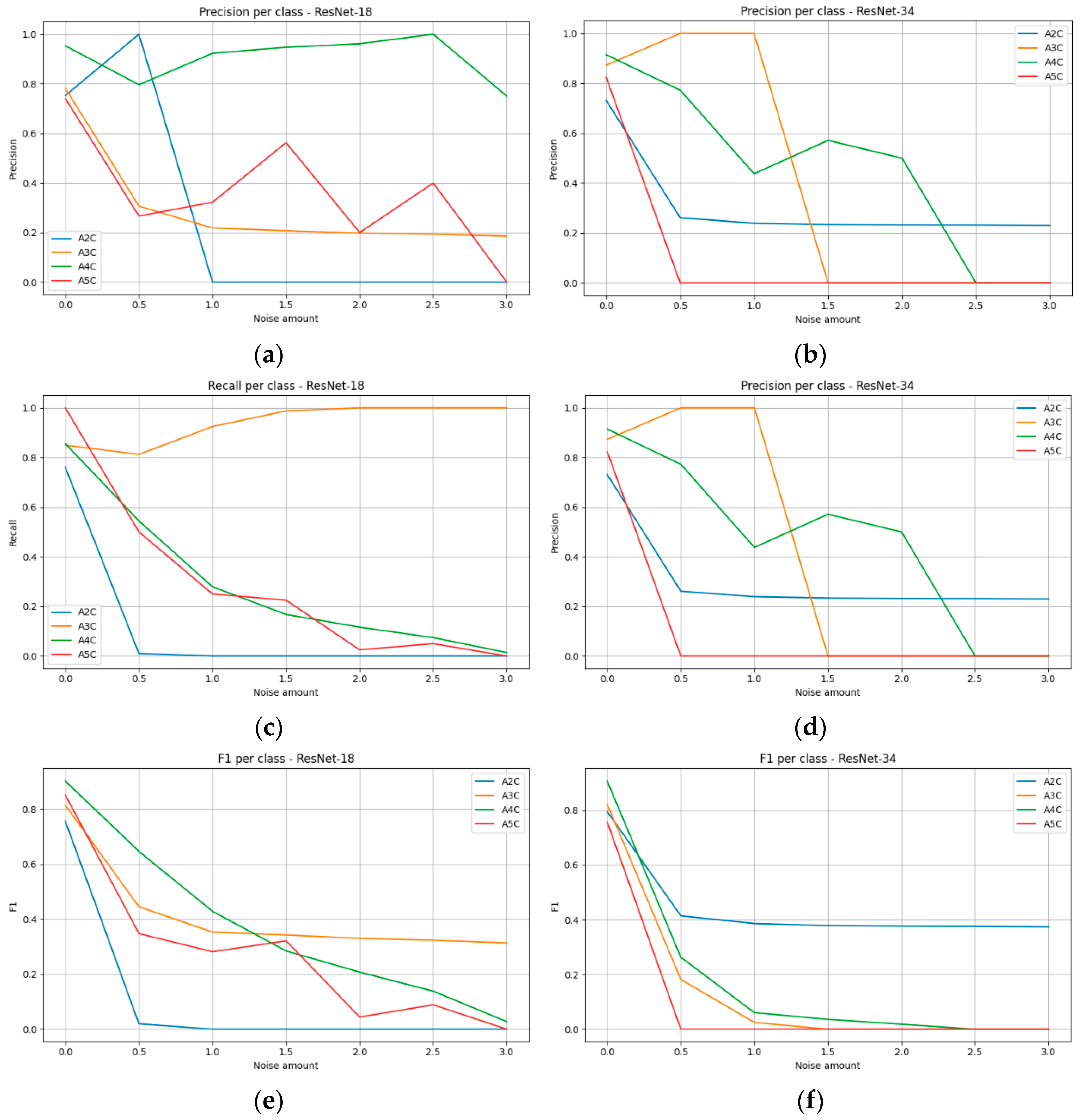
Impact of speckle noise on the classification performance of transthoracic echocardiographic (TTE) views for ResNet-18 and ResNet-34 models. Results are presented separately for precision (a,b), recall (c,d), and F1-score (e,f), broken down by projection classes: A2C, A3C, A4C, and A5C.
Figure 16.
Impact of speckle noise on the classification performance of transthoracic echocardiographic (TTE) views for ResNet-18 and ResNet-34 models. Results are presented separately for precision (a,b), recall (c,d), and F1-score (e,f), broken down by projection classes: A2C, A3C, A4C, and A5C.
Figure 17.
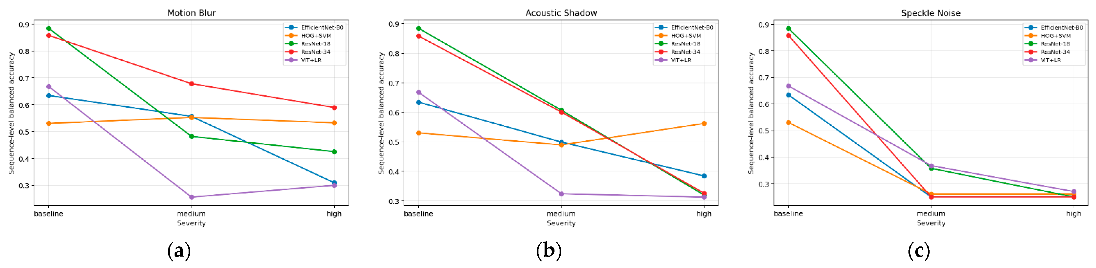
Comparison of sequence-level balanced accuracy for ResNet-18, ResNet-34, EfficientNet-B0, ViT + LR, and HOG + SVM as a function of artifact severity for: (a) motion blur, (b) acoustic shadowing, and (c) speckle noise.
Figure 17.
Comparison of sequence-level balanced accuracy for ResNet-18, ResNet-34, EfficientNet-B0, ViT + LR, and HOG + SVM as a function of artifact severity for: (a) motion blur, (b) acoustic shadowing, and (c) speckle noise.
Figure 18.
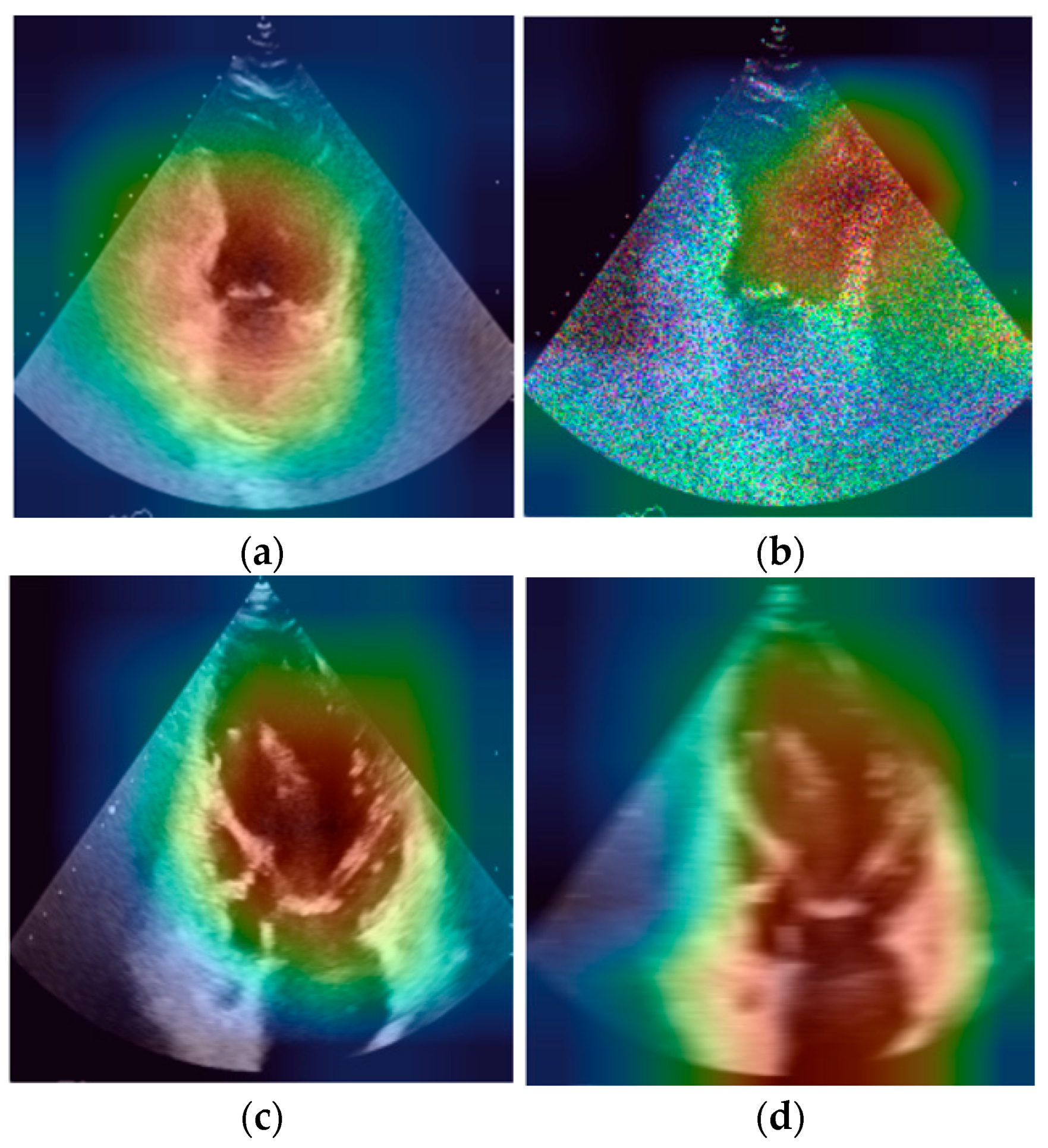
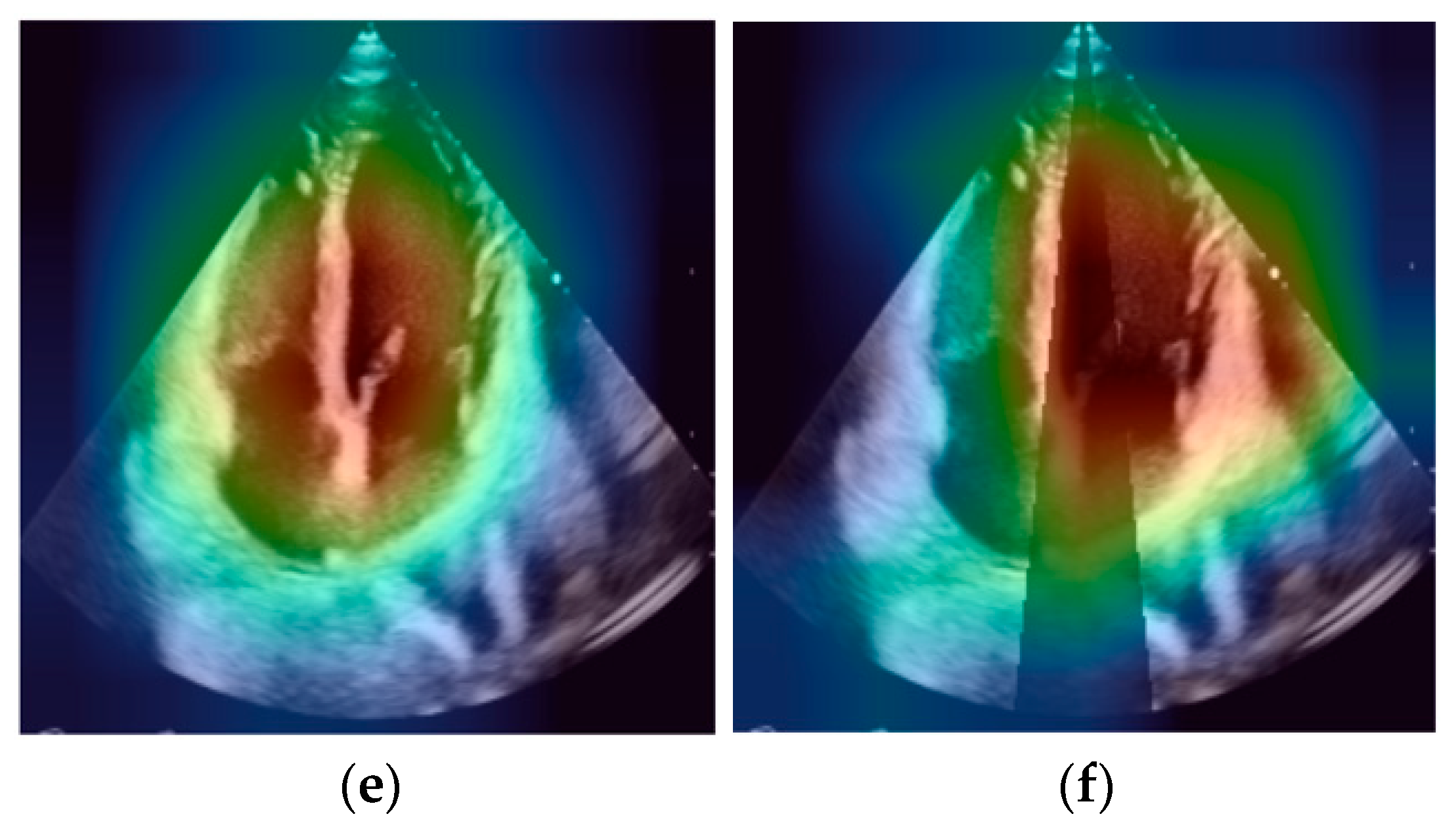
Grad-CAM visualization of CNN attention for baseline and artifact-degraded echocardiographic images. (a,c,e) Baseline images. (b,d,f) Corresponding images degraded by simulated artifacts: speckle noise (a,b), motion blur (c,d), and acoustic shadow (e,f). Warmer colors indicate image regions with higher Grad-CAM activation and stronger contribution to the model prediction, whereas cooler colors indicate regions with lower activation and weaker contribution.
Figure 18.
Grad-CAM visualization of CNN attention for baseline and artifact-degraded echocardiographic images. (a,c,e) Baseline images. (b,d,f) Corresponding images degraded by simulated artifacts: speckle noise (a,b), motion blur (c,d), and acoustic shadow (e,f). Warmer colors indicate image regions with higher Grad-CAM activation and stronger contribution to the model prediction, whereas cooler colors indicate regions with lower activation and weaker contribution.
Table 1.
Number of frames assigned to individual apical cardiac views in the training and test sets.
Table 1.
Number of frames assigned to individual apical cardiac views in the training and test sets.
| Projection | Frames in Training Set | Frames in Validation Set | Frames in Test Set |
|---|
| A2C | 334 | 84 | 100 |
| A3C | 248 | 62 | 80 |
| A4C | 688 | 172 | 215 |
| A5C | 119 | 28 | 40 |
Table 2.
Computational characteristics of the ResNet-18 and ResNet-34 architectures.
Table 2.
Computational characteristics of the ResNet-18 and ResNet-34 architectures.
| Model | Parameters [M] | FLOPs [G] | Inference Time [ms] |
|---|
| ResNet-18 | 11.18 | 4.74 | 22.08 |
| ResNet-34 | 21.29 | 9.57 | 40.65 |
Table 3.
Training configuration of the primary CNN models.
Table 3.
Training configuration of the primary CNN models.
| Parameter | Value |
|---|
| Architectures | ResNet-18, ResNet-34 (torchvision) |
| Pretraining | ImageNet-1K pretrained weights |
| Output head | Dropout (p = 0.3) + linear classification layer |
| Classes | A2C, A3C, A4C, A5C |
| Input resolution | 256 × 256 RGB images |
| Normalization | ImageNet statistics |
| Data augmentation | random rotation (±10°), horizontal flip |
| Train/test split | sequence-level stratified 80/20 |
| Validation split | frame-level stratified 20% of training data |
| Optimizer | AdamW |
| Learning rate | 1 × 10⁻⁴ (backbone), 5 × 10⁻⁴ (classification head) |
| Weight decay | 1 × 10⁻⁴ |
| Loss function | cross-entropy with label smoothing (0.05) |
| Class imbalance handling | class-weighted loss + weighted sampling |
| Batch size | 32 |
| Maximum epochs | 30 |
| Learning-rate scheduler | cosine annealing |
| Early stopping | patience = 5 epochs |
Table 4.
Training configuration of additional models.
Table 4.
Training configuration of additional models.
| Model | Initialization | Training Strategy | Feature Representation | Classifier |
|---|
| EfficientNet-B0 | ImageNet-1K pretrained | Full fine-tuning (same
protocol as ResNet models) | Final feature maps | Linear layer |
| ViT-B/16 | ImageNet-1K pretrained | Frozen backbone | CLS token embedding | Logistic Regression |
| HOG + SVM | HOG descriptor computed from grayscale images | no end-to-end training; handcrafted feature extraction | histograms of oriented gradients | Support Vector Machine |
Table 5.
Classification metrics (precision, recall, F1-score, AUC) for the ResNet-18 model under reference conditions.
Table 5.
Classification metrics (precision, recall, F1-score, AUC) for the ResNet-18 model under reference conditions.
| Projection | Precision | Recall | F1-Score | AUC | Support |
|---|
| A2C | 0.752 (0.666–0.836) | 0.760 (0.676–0.842) | 0.756 (0.687–0.824) | 0.951 (0.931–0.969) | 100 |
| A3C | 0.782 (0.691–0.871) | 0.850 (0.772–0.928) | 0.814 (0.744–0.878) | 0.974 (0.959–0.985) | 80 |
| A4C | 0.953 (0.923–0.979) | 0.856 (0.809–0.899) | 0.902 (0.869–0.93) | 0.962 (0.942–0.979) | 215 |
| A5C | 0.741 (0.625–0.843) | 1.000 (1.0–1.0) | 0.851 (0.769–0.914) | 0.998 (0.994–0.999) | 40 |
| accuracy | 0.846 | 435 |
| balanced accuracy | 0.866 |
Table 6.
Classification metrics (precision, recall, F1-score, AUC) for the ResNet-34 model under reference conditions.
Table 6.
Classification metrics (precision, recall, F1-score, AUC) for the ResNet-34 model under reference conditions.
| Projection | Precision | Recall | F1-Score | AUC | Support |
|---|
| A2C | 0.731 (0.648–0.809) | 0.870 (0.802–0.933) | 0.795 (0.728–0.848) | 0.959 (0.941–0.974) | 100 |
| A3C | 0.873 (0.794–0.945) | 0.775 (0.682–0.869) | 0.821 (0.748–0.887) | 0.983 (0.972–0.991) | 80 |
| A4C | 0.915 (0.876–0.949) | 0.898 (0.856–0.936) | 0.906 (0.877–0.931) | 0.956 (0.934–0.975) | 215 |
| A5C | 0.824 (0.687–0.942) | 0.7 (0.549–0.837) | 0.757 (0.631–0.857) | 0.965 (0.942–0.982) | 40 |
| accuracy | 0.851 | 435 |
| balanced accuracy | 0.81 |
Table 7.
Effect of motion blur intensity on Macro-AUC for the ResNet-18 model.
Table 7.
Effect of motion blur intensity on Macro-AUC for the ResNet-18 model.
| Motion Blur Kernel Size (k) | Baseline Macro-AUC | Macro-AUC Under Motion Blur | Δ AUC | 95% CI for Δ | Bootstrap p-Value | Holm-Adjusted p-Value | Significant (α = 0.05) |
|---|
| 0 | 0.981 | 0.981 | 0.000 | [0.000, 0.000] | 1.000 | 1.000 | No |
| 2.5 | 0.972 | −0.009 | [−0.027, 0.004] | 0.186 | 0.372 | No |
| 5 | 0.947 | −0.034 | [−0.072, −0.005] | 0.006 | 0.018 | Yes |
| 7.5 | 0.905 | −0.076 | [−0.143, −0.024] | 0.000 | 0.000 | Yes |
| 10 | 0.876 | −0.106 | [−0.183, −0.038] | 0.000 | 0.000 | Yes |
| 12.5 | 0.841 | −0.140 | [−0.237, −0.052] | 0.000 | 0.000 | Yes |
| 15 | 0.813 | −0.168 | [−0.289, −0.061] | 0.000 | 0.000 | Yes |
| 17.5 | 0.765 | −0.216 | [−0.344, −0.096] | 0.000 | 0.000 | Yes |
| 20 | 0.757 | −0.224 | [−0.359, −0.099] | 0.000 | 0.000 | Yes |
Table 8.
Effect of motion blur intensity on Macro-AUC for the ResNet-34 model.
Table 8.
Effect of motion blur intensity on Macro-AUC for the ResNet-34 model.
| Motion Blur Kernel Size (k) | Baseline Macro-AUC | Macro-AUC Under Motion Blur | Δ AUC | 95% CI for Δ | Bootstrap p-Value | Holm-Adjusted p-Value | Significant (α = 0.05) |
|---|
| 0 | 0.976 | 0.976 | 0.000 | [0.000, 0.000] | 1.000 | 1.000 | No |
| 2.5 | 0.971 | −0.005 | [−0.021, 0.005] | 0.506 | 1.000 | No |
| 5 | 0.968 | −0.008 | [−0.025, 0.003] | 0.212 | 0.637 | No |
| 7.5 | 0.941 | −0.035 | [−0.080, −0.003] | 0.016 | 0.065 | No |
| 10 | 0.926 | −0.050 | [−0.101, −0.009] | 0.004 | 0.020 | Yes |
| 12.5 | 0.908 | −0.068 | [−0.132, −0.017] | 0.000 | 0.000 | Yes |
| 15 | 0.895 | −0.081 | [−0.151, −0.021] | 0.000 | 0.000 | Yes |
| 17.5 | 0.875 | −0.101 | [−0.171, −0.040] | 0.000 | 0.000 | Yes |
| 20 | 0.864 | −0.112 | [−0.189, −0.047] | 0.000 | 0.000 | Yes |
Table 9.
Effect of acoustic shadow width on Macro-AUC for the ResNet-18 model.
Table 9.
Effect of acoustic shadow width on Macro-AUC for the ResNet-18 model.
| Shadow Width Fraction | Baseline Macro-AUC | Macro-AUC Under Shadow | Δ AUC | 95% CI for Δ | Bootstrap p-Value | Holm-Adjusted p-Value | Significant (α = 0.05) |
|---|
| 0 | 0.981 | 0.981 | 0.000 | [0.000, 0.000] | 1.000 | 1.000 | No |
| 0.1 | 0.957 | −0.025 | [−0.053, 0.000] | 0.057 | 0.113 | No |
| 0.2 | 0.932 | −0.049 | [−0.105, −0.008] | 0.000 | 0.000 | Yes |
| 0.3 | 0.909 | −0.073 | [−0.141, −0.018] | 0.000 | 0.000 | Yes |
| 0.4 | 0.858 | −0.123 | [−0.224, −0.037] | 0.000 | 0.000 | Yes |
| 0.5 | 0.810 | −0.171 | [−0.276, −0.084] | 0.000 | 0.000 | Yes |
| 0.6 | 0.801 | −0.181 | [−0.279, −0.094] | 0.000 | 0.000 | Yes |
| 0.7 | 0.780 | −0.201 | [−0.306, −0.105] | 0.000 | 0.000 | Yes |
Table 10.
Effect of acoustic shadow width on Macro-AUC for the ResNet-34 model.
Table 10.
Effect of acoustic shadow width on Macro-AUC for the ResNet-34 model.
| Shadow Width Fraction | Baseline Macro-AUC | Macro-AUC Under Shadow | Δ AUC | 95% CI for Δ | Bootstrap p-Value | Holm-Adjusted p-Value | Significant (α = 0.05) |
|---|
| 0 | 0.976 | 0.976 | 0.000 | [0.000, 0.000] | 1.000 | 1.000 | No |
| 0.1 | 0.951 | −0.025 | [−0.062, −0.003] | 0.028 | 0.057 | No |
| 0.2 | 0.905 | −0.071 | [−0.139, −0.022] | 0.000 | 0.000 | Yes |
| 0.3 | 0.914 | −0.062 | [−0.122, −0.019] | 0.000 | 0.000 | Yes |
| 0.4 | 0.871 | −0.105 | [−0.184, −0.045] | 0.000 | 0.000 | Yes |
| 0.5 | 0.828 | −0.148 | [−0.246, −0.069] | 0.000 | 0.000 | Yes |
| 0.6 | 0.798 | −0.178 | [−0.286, −0.090] | 0.000 | 0.000 | Yes |
| 0.7 | 0.847 | −0.129 | [−0.202, −0.068] | 0.000 | 0.000 | Yes |
Table 11.
Effect of speckle noise intensity on Macro-AUC for the ResNet-18 model.
Table 11.
Effect of speckle noise intensity on Macro-AUC for the ResNet-18 model.
| Noise Amount | Baseline Macro-AUC | Macro-AUC Under Noise | Δ AUC | 95% CI for Δ | Bootstrap p-Value | Holm-Adjusted p-Value | Significant (α = 0.05) |
|---|
| 0 | 0.981 | 0.981 | 0.000 | [0.000, 0.000] | 1.000 | 1.000 | No |
| 0.5 | 0.832 | −0.149 | [−0.231, −0.077] | 0.000 | 0.000 | Yes |
| 1 | 0.768 | −0.213 | [−0.306, −0.123] | 0.000 | 0.000 | Yes |
| 1.5 | 0.706 | −0.275 | [−0.387, −0.165] | 0.000 | 0.000 | Yes |
| 2 | 0.691 | −0.290 | [−0.411, −0.172] | 0.000 | 0.000 | Yes |
| 2.5 | 0.684 | −0.297 | [−0.408, −0.184] | 0.000 | 0.000 | Yes |
| 3 | 0.663 | −0.319 | [−0.445, −0.196] | 0.000 | 0.000 | Yes |
Table 12.
Effect of speckle noise intensity on Macro-AUC for the ResNet-34 model.
Table 12.
Effect of speckle noise intensity on Macro-AUC for the ResNet-34 model.
| Noise Amount | Baseline Macro-AUC | Macro-AUC Under Noise | Δ AUC | 95% CI for Δ | Bootstrap p-Value | Holm-Adjusted p-Value | Significant (α = 0.05) |
|---|
| 0 | 0.976 | 0.976 | 0.000 | [0.000, 0.000] | 1.000 | 1.000 | No |
| 0.5 | 0.900 | −0.076 | [−0.131, −0.028] | 0.000 | 0.000 | Yes |
| 1 | 0.690 | −0.286 | [−0.375, −0.187] | 0.000 | 0.000 | Yes |
| 1.5 | 0.634 | −0.342 | [−0.443, −0.242] | 0.000 | 0.000 | Yes |
| 2 | 0.588 | −0.388 | [−0.493, −0.295] | 0.000 | 0.000 | Yes |
| 2.5 | 0.575 | −0.401 | [−0.515, −0.288] | 0.000 | 0.000 | Yes |
| 3 | 0.591 | −0.385 | [−0.500, −0.261] | 0.000 | 0.000 | Yes |
Table 13.
Comparison of sequence-level balanced accuracy for the primary and reference models under reference conditions and under medium and high levels of simulated artifacts.
Table 13.
Comparison of sequence-level balanced accuracy for the primary and reference models under reference conditions and under medium and high levels of simulated artifacts.
| Model | Baseline | Motion Blur (10) | Motion Blur (20) | Acoustic Shadow (0.3) | Acoustic Shadow (0.7) | Speckle Noise (1.5) | Speckle Noise (3.0) |
|---|
| ResNet-18 | 0.885 | 0.482 | 0.426 | 0.607 | 0.320 | 0.358 | 0.250 |
| ResNet-34 | 0.859 | 0.678 | 0.590 | 0.601 | 0.326 | 0.250 | 0.250 |
| EfficientNet-B0 | 0.635 | 0.557 | 0.310 | 0.499 | 0.385 | 0.250 | 0.250 |
| ViT + LR | 0.668 | 0.256 | 0.300 | 0.324 | 0.313 | 0.368 | 0.270 |
| HOG + SVM | 0.531 | 0.553 | 0.533 | 0.490 | 0.562 | 0.261 | 0.261 |
Table 14.
Representative failure cases illustrating systematic misclassification under image artifacts.
Table 14.
Representative failure cases illustrating systematic misclassification under image artifacts.
| Model | Artifact Type | Intensity | True View | Predicted View | Δ True-Class Probability |
|---|
| ResNet-18 | Motion blur | kernel = 5.0 | A5C | A3C | −0.88 |
| ResNet-18 | Acoustic shadow | wf = 0.7 | A5C | A2C | −0.65 |
| ResNet-18 | Speckle noise | Speckle = 3.0 | A5C | A2C | −0.77 |
| ResNet-34 | Motion blur | kernel = 2.5 | A2C | A3C | −0.89 |
| ResNet-34 | Acoustic shadow | Wf = 0.6 | A2C | A3C | −0.75 |
| ResNet-34 | Speckle noise | Speckle =2.5 | A3C | A2C | −0.89 |
Table 15.
Checklist of evaluation criteria for the proposed echocardiographic view classification framework.
Table 15.
Checklist of evaluation criteria for the proposed echocardiographic view classification framework.
| Criterion | Description | Addressed in This Study |
|---|
| Baseline performance | Classification accuracy and discrimination under reference (artifact-free) imaging conditions | Section 3.1, Figure 9 |
| Robustness to artifacts | Performance degradation under controlled motion blur, acoustic shadowing, speckle noise, etc. | Section 3.2, Section 3.3, Section 3.4 and Section 3.5; Table 5, Table 6, Table 7, Table 8, Table 9, Table 10, Table 11 and Table 12 |
| Probability stability | Changes in true-class probability distributions with increasing artifact severity | Section 3.7, Table 14 |
| Architectural consistency | Comparison of degradation trends across ResNet-18 and ResNet-34 | Section 3.2, Section 3.3, Section 3.4 and Section 3.5 |
| Failure mode transparency | Qualitative analysis of systematic misclassifications under artifacts | Section 3.8 |



 ,
,