

Controlling Cell Migratory Patterns Under an Electric Field Regulated by a Neural Network-Based Feedback Controller

 ,
,  , , , , and
Abstract
1. Introduction
2. Materials and Methods
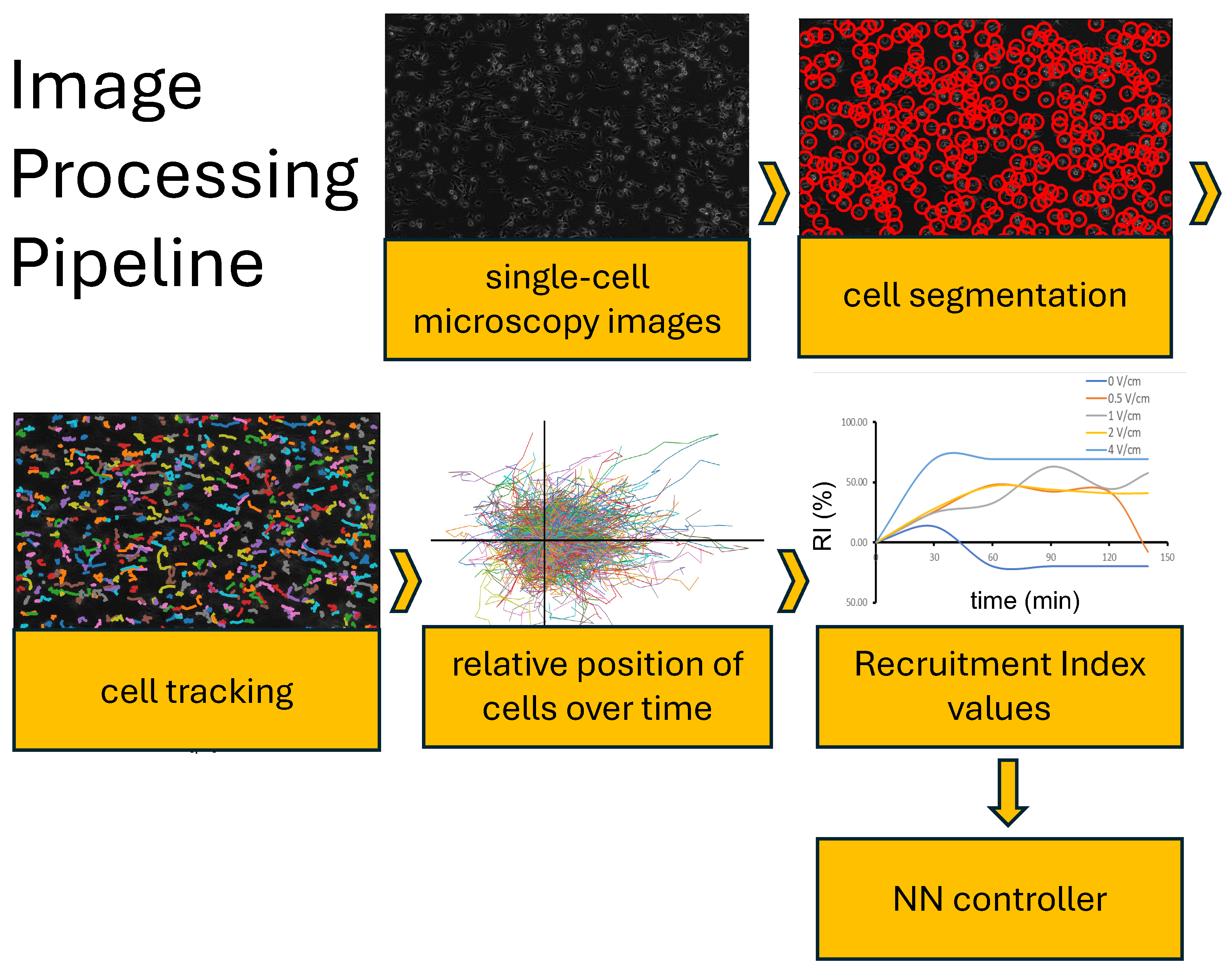
2.1. Image Analysis Tool for Image Processing/Cell Tracking
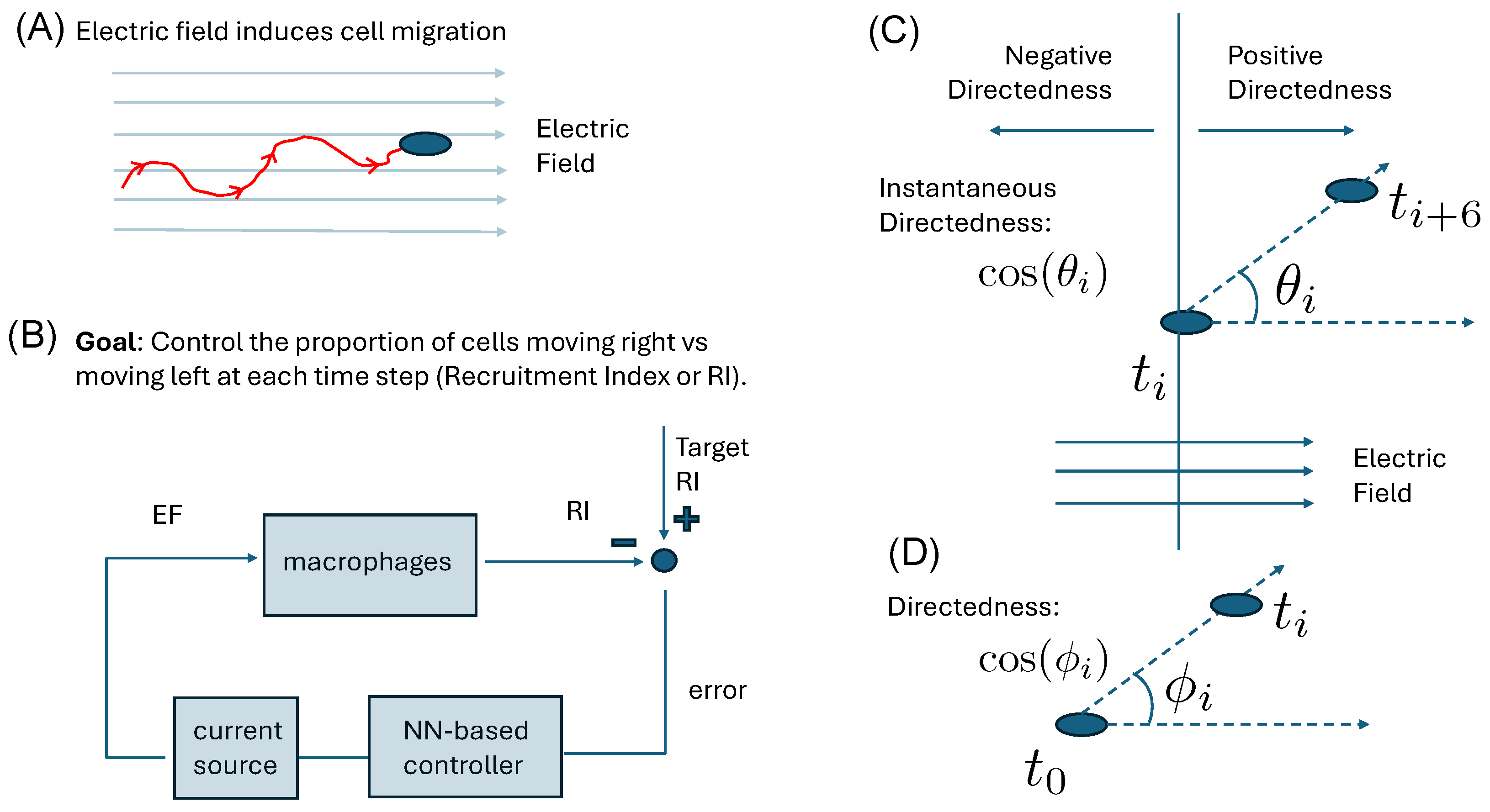
2.2. Quantification of Cellular Response
- are those cells with directedness .
- are those cells with directedness .
- is the total cell count (including those with directedness between and ).
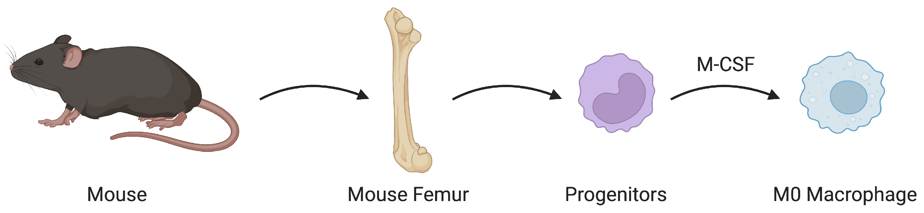
2.3. Preparing Macrophages
2.4. Experimental Setup
2.5. Neural Network Controller Overview
3. Results
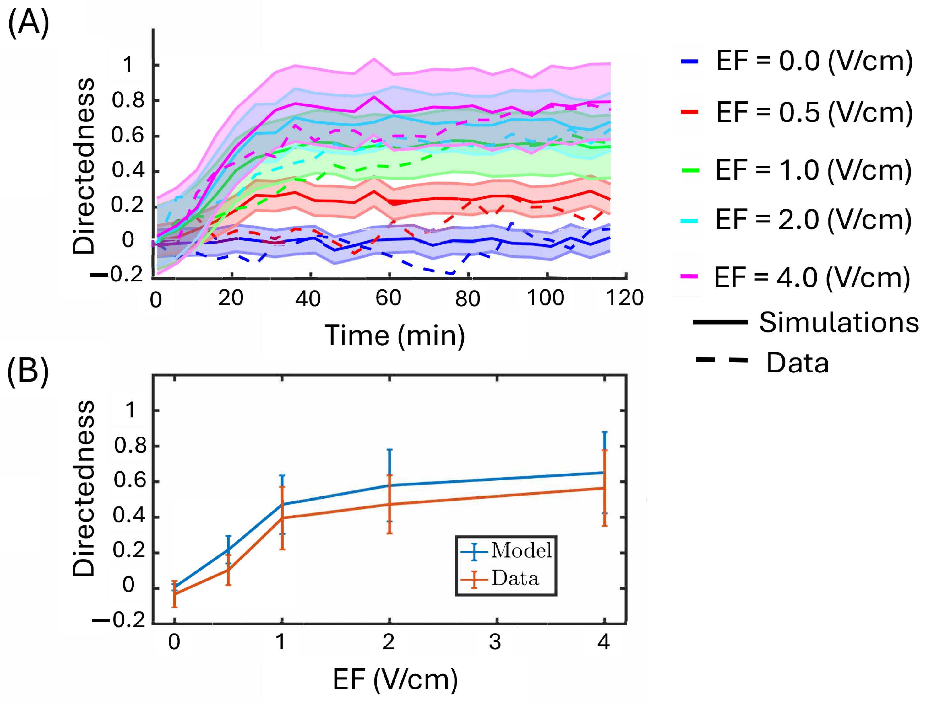
3.1. Qualitative Stochastic Model of Cell Directedness
3.2. Adapted Neural Network Controller
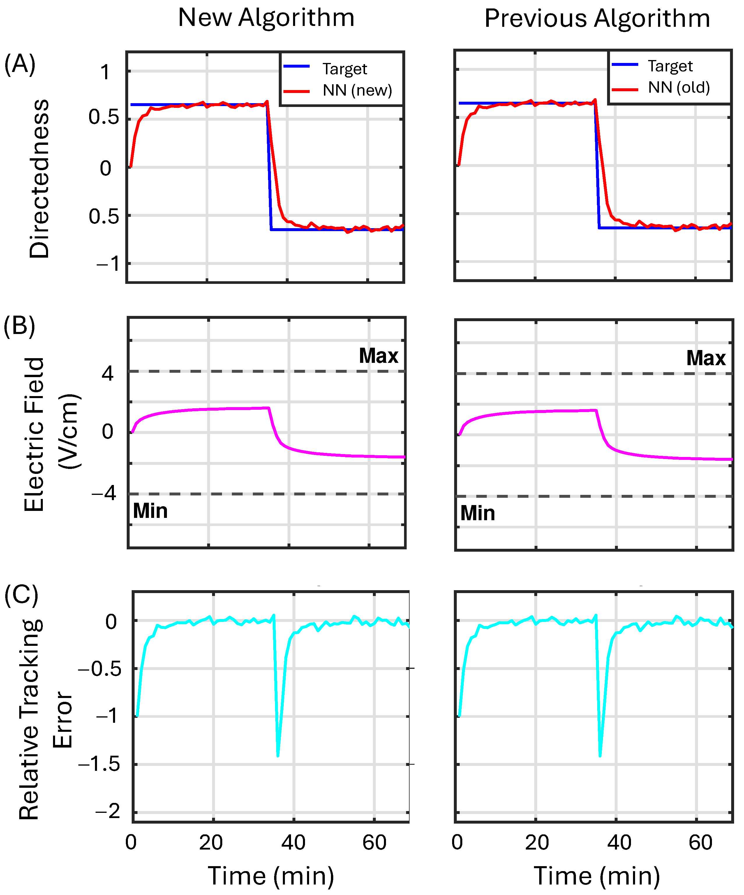
3.3. In Silico Feedback Control Experiments
3.3.1. Example 1
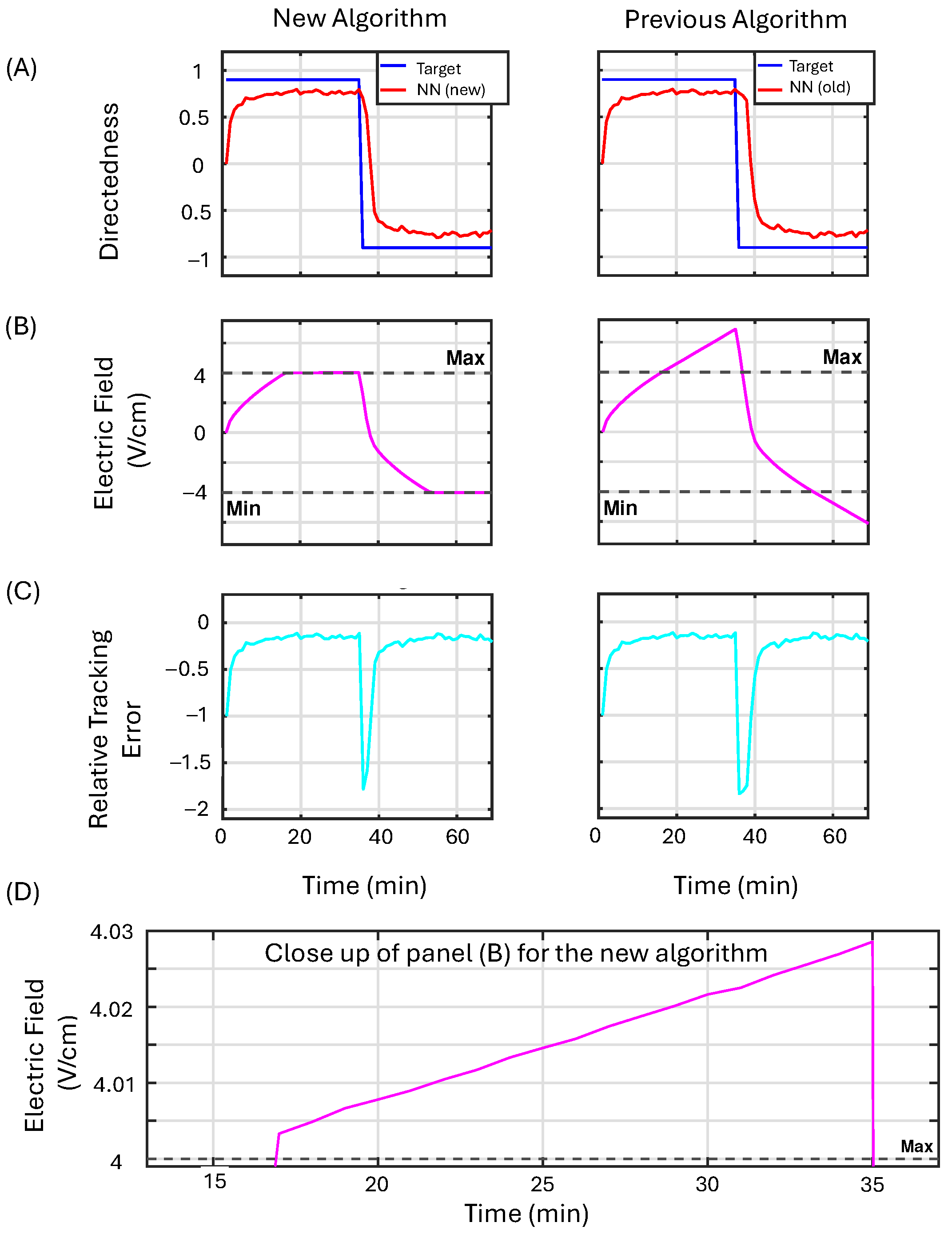
3.3.2. Example 2
3.3.3. Example 3
3.3.4. Summary
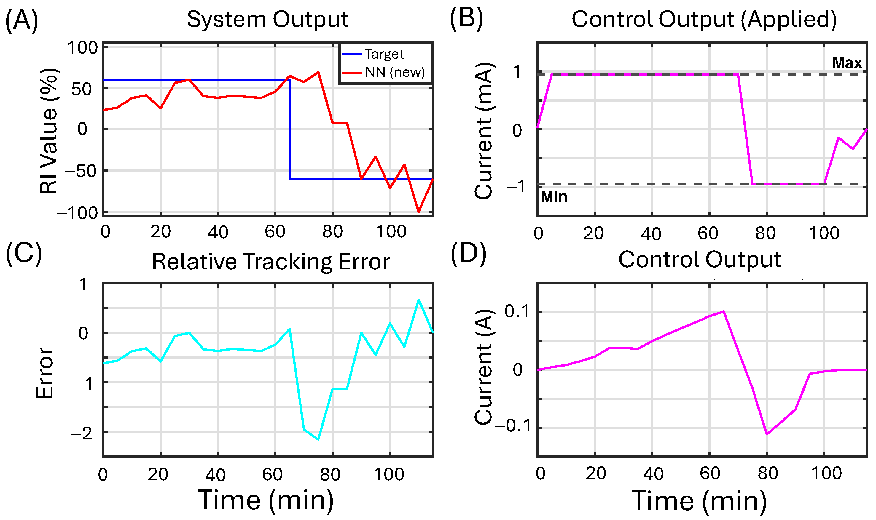
3.4. In Vitro Feedback Control Experiments
4. Discussion
5. Conclusions
Author Contributions
Funding
Institutional Review Board Statement
Informed Consent Statement
Data Availability Statement
Acknowledgments
Conflicts of Interest
Appendix A. Lyapunov Analysis
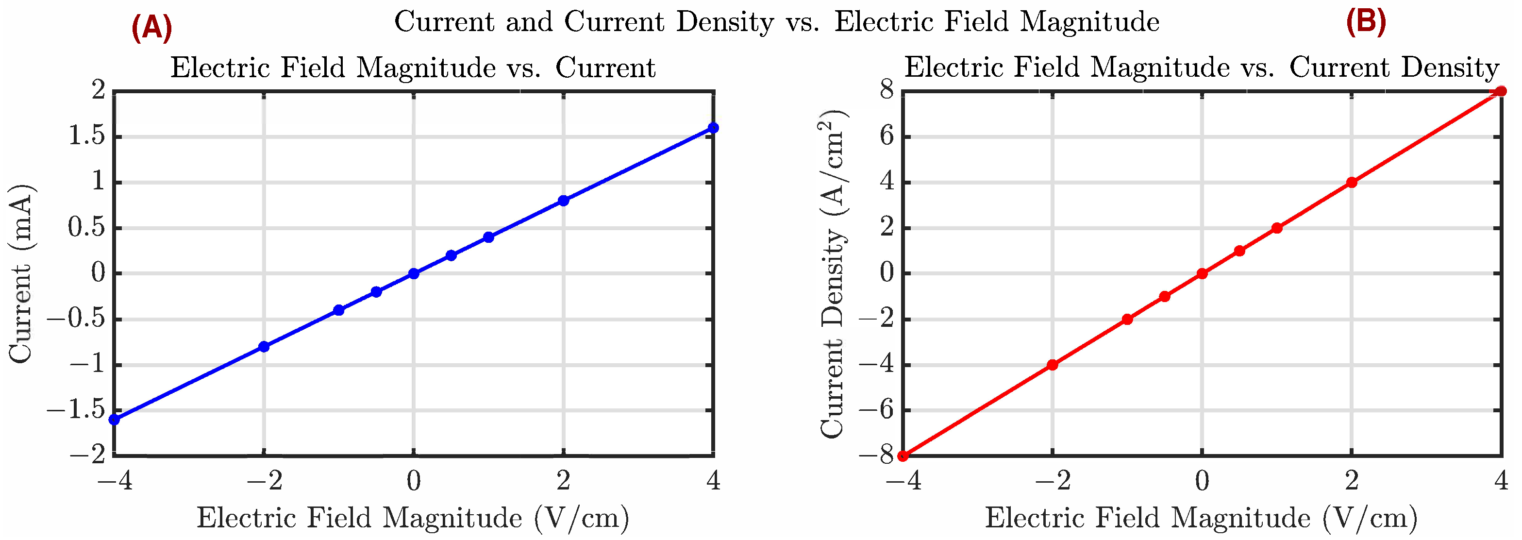
Appendix B. Electric Field, Current Density, and Current Relations
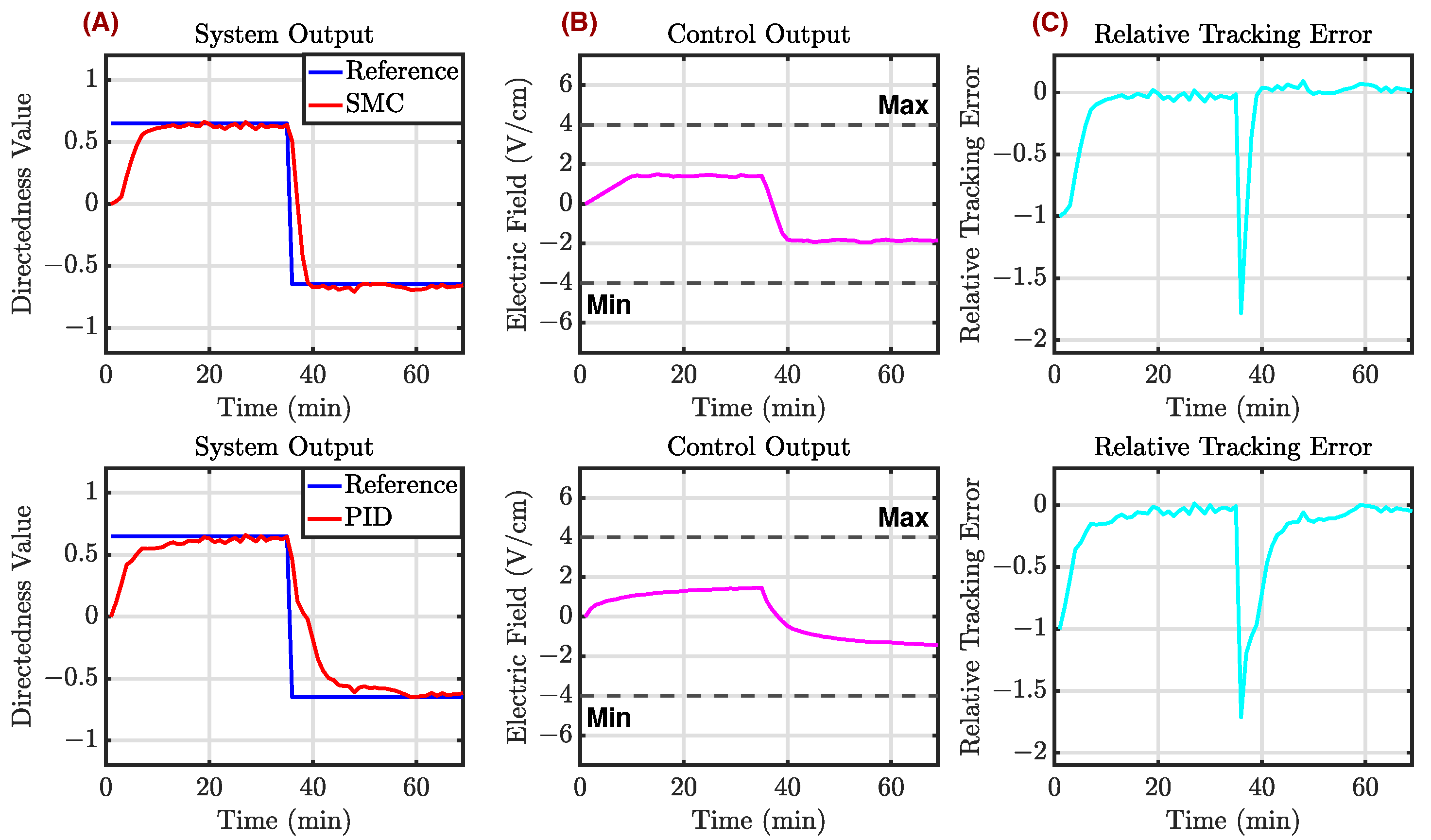
Appendix C. Additional In Silico Comparisons with Existing Controllers
Appendix C.1. Example 1
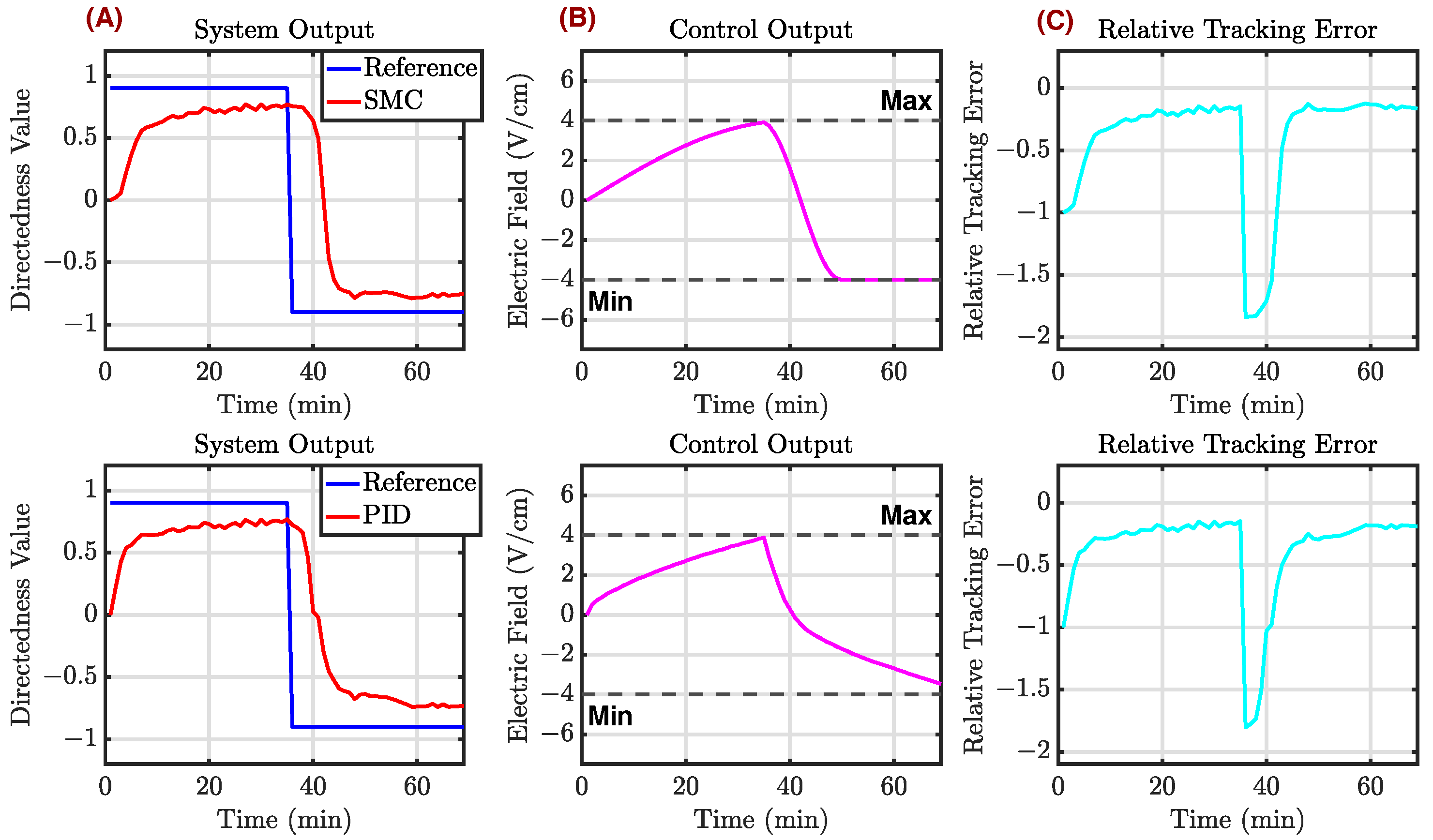
Appendix C.2. Example 2
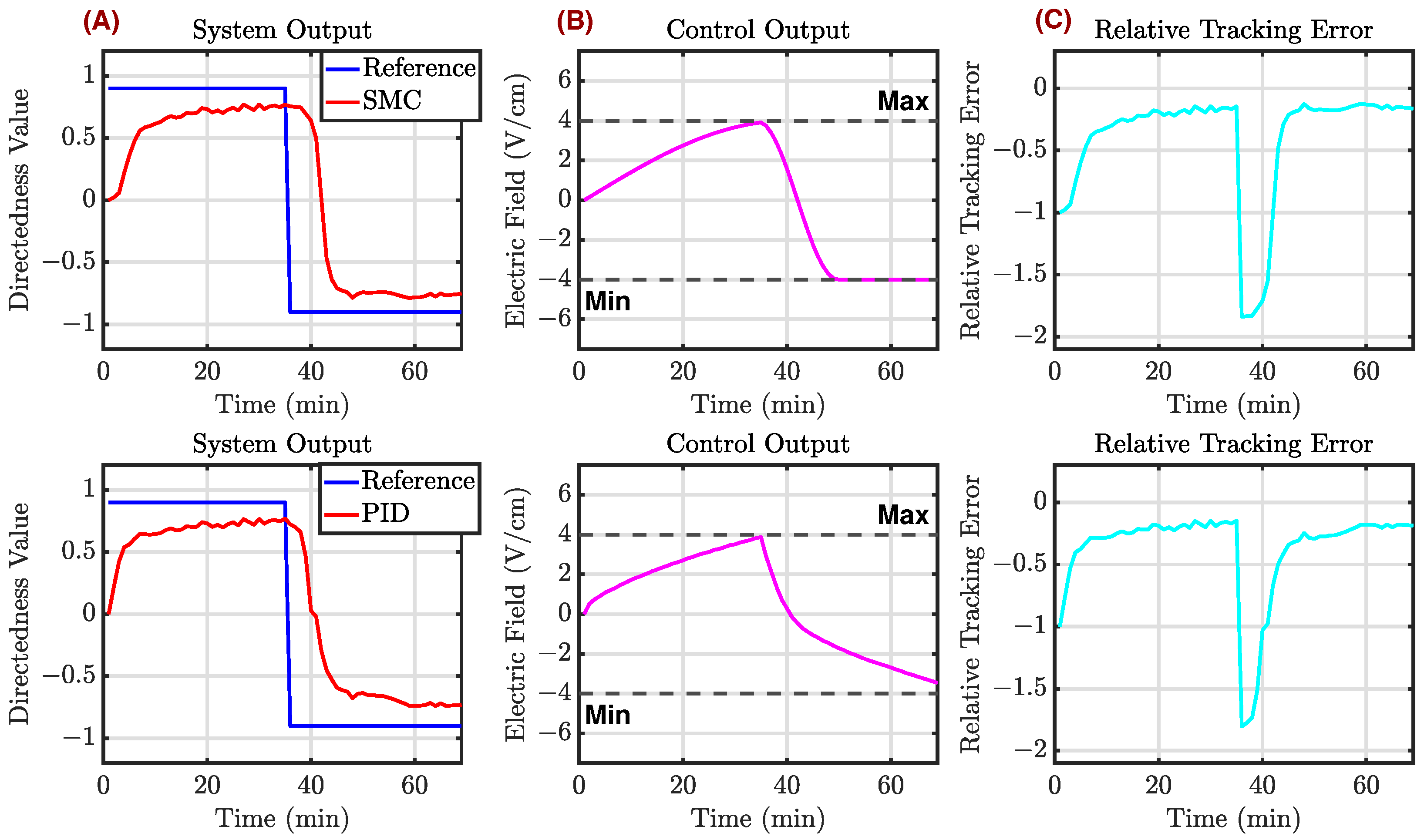
Appendix C.3. Example 3

| Example 1 | Example 2 | Example 3 | |||||||
|---|---|---|---|---|---|---|---|---|---|
| Controller | MSE | RMSE | MAPE | MSE | RMSE | MAPE | MSE | RMSE | MAPE |
| 0.0339 | 0.1841 | 10.7568 | 0.1230 | 0.3507 | 25.5900 | 0.1265 | 0.3556 | 25.8044 | |
| 0.0540 | 0.2324 | 14.4509 | 0.3161 | 0.5622 | 40.3215 | 0.3161 | 0.5622 | 40.3215 | |
| 0.0657 | 0.2563 | 20.6002 | 0.2397 | 0.4895 | 37.9279 | 0.2397 | 0.4895 | 37.9279 | |
References
- Vicente-Manzanares, M.; Horwitz, A.R. Cell migration: An overview. Cell Migr. 2011, 769, 1–24. [Google Scholar]
- Zlobina, K.; Jafari, M.; Rolandi, M.; Gomez, M. The role of machine learning in advancing precision medicine with feedback control. Cell Rep. Phys. Sci. 2022, 3, 101149. [Google Scholar] [CrossRef]
- Selberg, J.; Jafari, M.; Bradley, C.; Gomez, M.; Rolandi, M. Expanding biological control to bioelectronics with machine learning. APL Mater. 2020, 8, 120904. [Google Scholar] [CrossRef]
- Owens, R.; Kjall, P.; Richter-Dahlfors, A.; Cicoira, F. Organic bioelectronics-novel applications in biomedicine. Preface. Biochim. Biophys. Acta 2013, 1830, 4283–4285. [Google Scholar] [CrossRef]
- Griffin, M.F.; Butler, P.E.; Seifalian, A.M.; Kalaskar, D.M. Control of stem cell fate by engineering their micro and nanoenvironment. World J. Stem Cells 2015, 7, 37. [Google Scholar] [CrossRef]
- Simon, D.T.; Gabrielsson, E.O.; Tybrandt, K.; Berggren, M. Organic bioelectronics: Bridging the signaling gap between biology and technology. Chem. Rev. 2016, 116, 13009–13041. [Google Scholar] [CrossRef]
- Strakosas, X.; Seitanidou, M.; Tybrandt, K.; Berggren, M.; Simon, D.T. An electronic proton-trapping ion pump for selective drug delivery. Sci. Adv. 2021, 7, eabd8738. [Google Scholar] [CrossRef] [PubMed]
- Zhao, M. Electrical fields in wound healing—An overriding signal that directs cell migration. In Seminars in Cell & Developmental Biology; Elsevier: Amsterdam, The Netherlands, 2009; Volume 20, pp. 674–682. [Google Scholar]
- Shaner, S.; Savelyeva, A.; Kvartuh, A.; Jedrusik, N.; Matter, L.; Leal, J.; Asplund, M. Bioelectronic microfluidic wound healing: A platform for investigating direct current stimulation of injured cell collectives. Lab Chip 2023, 23, 1531–1546. [Google Scholar] [CrossRef] [PubMed]
- Shirzaei Sani, E.; Xu, C.; Wang, C.; Song, Y.; Min, J.; Tu, J.; Solomon, S.A.; Li, J.; Banks, J.L.; Armstrong, D.G.; et al. A stretchable wireless wearable bioelectronic system for multiplexed monitoring and combination treatment of infected chronic wounds. Sci. Adv. 2023, 9, eadf7388. [Google Scholar] [CrossRef]
- Jiang, Y.; Trotsyuk, A.A.; Niu, S.; Henn, D.; Chen, K.; Shih, C.C.; Larson, M.R.; Mermin-Bunnell, A.M.; Mittal, S.; Lai, J.C.; et al. Wireless closed-loop smart bandage for chronic wound management and accelerated tissue regeneration. bioRxiv 2022. [Google Scholar] [CrossRef]
- Mycielska, M.E.; Djamgoz, M.B. Cellular mechanisms of direct-current electric field effects: Galvanotaxis and metastatic disease. J. Cell Sci. 2004, 117, 1631–1639. [Google Scholar] [CrossRef] [PubMed]
- Sargent, B.; Jafari, M.; Marquez, G.; Mehta, A.S.; Sun, Y.H.; Yang, H.y.; Zhu, K.; Isseroff, R.R.; Zhao, M.; Gomez, M. A machine learning based model accurately predicts cellular response to electric fields in multiple cell types. Sci. Rep. 2022, 12, 1–13. [Google Scholar] [CrossRef] [PubMed]
- Zajdel, T.J.; Shim, G.; Wang, L.; Rossello-Martinez, A.; Cohen, D.J. SCHEEPDOG: Programming electric cues to dynamically herd large-scale cell migration. Cell Syst. 2020, 10, 506–514. [Google Scholar] [CrossRef]
- Hoare, J.I.; Rajnicek, A.M.; McCaig, C.D.; Barker, R.N.; Wilson, H.M. Electric fields are novel determinants of human macrophage functions. J. Leucoc. Biol. 2016, 99, 1141–1151. [Google Scholar] [CrossRef] [PubMed]
- Xue, J.D.; Gao, J.; Tang, A.F.; Feng, C. Shaping the immune landscape: Multidimensional environmental stimuli refine macrophage polarization and foster revolutionary approaches in tissue regeneration. Heliyon 2024, 10, e37192. [Google Scholar] [CrossRef]
- Lillacci, G.; Khammash, M. Parameter estimation and model selection in computational biology. PLoS Comput. Biol. 2010, 6, e1000696. [Google Scholar] [CrossRef]
- Eisner, V.; Picard, M.; Hajnóczky, G. Mitochondrial dynamics in adaptive and maladaptive cellular stress responses. Nat. Cell Biol. 2018, 20, 755–765. [Google Scholar] [CrossRef]
- Jafari, M.; Marquez, G.; Selberg, J.; Jia, M.; Dechiraju, H.; Pansodtee, P.; Teodorescu, M.; Rolandi, M.; Gomez, M. Feedback Control of Bioelectronic Devices Using Machine Learning. IEEE Control Syst. Lett. 2020, 5, 1133–1138. [Google Scholar] [CrossRef]
- Hosseini Jafari, B.; Zlobina, K.; Marquez, G.; Jafari, M.; Selberg, J.; Jia, M.; Rolandi, M.; Gomez, M. A feedback control architecture for bioelectronic devices with applications to wound healing. J. R. Soc. Interface 2021, 18, 20210497. [Google Scholar] [CrossRef]
- Allan, D.B.; Caswell, T.; Keim, N.C.; van der Wel, C.M.; Verweij, R.W. Soft-Matter/Trackpy: Trackpy v0. 5.0. Zenodo Repository 2021. Available online: https://zenodo.org/records/4682814 (accessed on 19 May 2022).
- Sun, Y.; Luxardi, G.; Xu, G.; Zhu, K.; Reid, B.; Guo, B.; Lebrilla, C.; Maverakis, E.; Zhao, M. Surface Glycans Regulate Salmonella Infection-Dependent Directional Switch in Macrophage Galvanotaxis Independent of NanH. Infect. Immun. 2022, 90, e00516-21. [Google Scholar] [CrossRef]
- Song, B.; Gu, Y.; Pu, J.; Reid, B.; Zhao, Z.; Zhao, M. Application of direct current electric fields to cells and tissues in vitro and modulation of wound electric field in vivo. Nat. Protoc. 2007, 2, 1479–1489. [Google Scholar] [CrossRef] [PubMed]
- Marquez, G.; Johnson, B.; Jafari, M.; Gomez, M. Online machine learning based predictor for biological systems. In Proceedings of the 2019 IEEE Symposium Series on Computational Intelligence (SSCI), Xiamen, China, 6–9 December 2019; pp. 120–125. [Google Scholar]
- Kang, H.; Kim, S.; Wong, D.S.H.; Jung, H.J.; Lin, S.; Zou, K.; Li, R.; Li, G.; Dravid, V.P.; Bian, L. Remote manipulation of ligand nano-oscillations regulates adhesion and polarization of macrophages in vivo. Nano Lett. 2017, 17, 6415–6427. [Google Scholar] [CrossRef]
- Bianconi, S.; Leppik, L.; Oppermann, E.; Marzi, I.; Henrich, D. Direct Current Electrical Stimulation Shifts THP-1-Derived Macrophage Polarization towards Pro-Regenerative M2 Phenotype. Int. J. Mol. Sci. 2024, 25, 7272. [Google Scholar] [CrossRef]
- Gu, J.; Wu, C.; He, X.; Chen, X.; Dong, L.; Weng, W.; Cheng, K.; Wang, D.; Chen, Z. Enhanced M2 polarization of oriented macrophages on the P (Vdf-Trfe) film by coupling with electrical stimulation. ACS Biomater. Sci. Eng. 2023, 9, 2615–2624. [Google Scholar] [CrossRef] [PubMed]
- Kim, S.Y.; Nair, M.G. Macrophages in wound healing: Activation and plasticity. Immunol. Cell Biol. 2019, 97, 258–267. [Google Scholar] [CrossRef]
- Zlobina, K.; Xue, J.; Gomez, M. Effective spatio-temporal regimes for wound treatment by way of macrophage polarization: A mathematical model. Front. Appl. Math. Stat. 2022, 8, 791064. [Google Scholar] [CrossRef]
- Kesapragada, M.; Sun, Y.H.; Zhu, K.; Recendez, C.; Fregoso, D.; Yang, H.Y.; Rolandi, M.; Isseroff, R.; Zhao, M.; Gomez, M. A data-driven approach to establishing cell motility patterns as predictors of macrophage subtypes and their relation to cell morphology. PLoS ONE 2024, 19, e0315023. [Google Scholar] [CrossRef]
- Kesapragada, M.; Sun, Y.H.; Zlobina, K.; Recendez, C.; Fregoso, D.; Yang, H.Y.; Aslankoohi, E.; Isseroff, R.; Rolandi, M.; Zhao, M.; et al. Deep learning classification for macrophage subtypes through cell migratory pattern analysis. Front. Cell Dev. Biol. 2024, 12, 1259037. [Google Scholar] [CrossRef]
- Mao, J.; Chen, L.; Cai, Z.; Qian, S.; Liu, Z.; Zhao, B.; Zhang, Y.; Sun, X.; Cui, W. Advanced biomaterials for regulating polarization of macrophages in wound healing. Adv. Funct. Mater. 2022, 32, 2111003. [Google Scholar] [CrossRef]
- Sun, Y.; Reid, B.; Ferreira, F.; Luxardi, G.; Ma, L.; Lokken, K.L.; Zhu, K.; Xu, G.; Sun, Y.; Ryzhuk, V.; et al. Infection-generated electric field in gut epithelium drives bidirectional migration of macrophages. PLoS Biol. 2019, 17, e3000044. [Google Scholar] [CrossRef]
- Kulkarni, S.; Tebar, F.; Rentero, C.; Zhao, M.; Saez, P. Competing signaling pathways controls electrotaxis. bioRxiv 2025. [Google Scholar] [CrossRef] [PubMed]
- Zhao, M.; Song, B.; Pu, J.; Wada, T.; Reid, B.; Tai, G.; Wang, F.; Guo, A.; Walczysko, P.; Gu, Y.; et al. Electrical signals control wound healing through phosphatidylinositol-3-OH kinase-γ and PTEN. Nature 2006, 442, 457–460. [Google Scholar] [CrossRef] [PubMed]
- Li, L.; Zhang, K.; Lu, C.; Sun, Q.; Zhao, S.; Jiao, L.; Han, R.; Lin, C.; Jiang, J.; Zhao, M.; et al. Caveolin-1-mediated STAT3 activation determines electrotaxis of human lung cancer cells. Oncotarget 2017, 8, 95741. [Google Scholar] [CrossRef] [PubMed]
- Sun, Y.; Do, H.; Gao, J.; Zhao, R.; Zhao, M.; Mogilner, A. Keratocyte fragments and cells utilize competing pathways to move in opposite directions in an electric field. Curr. Biol. 2013, 23, 569–574. [Google Scholar] [CrossRef]
- Barabás, G.; Michalska-Smith, M.J.; Allesina, S. Self-regulation and the stability of large ecological networks. Nat. Ecol. Evol. 2017, 1, 1870–1875. [Google Scholar] [CrossRef]
- Korthuis, R.J. Skeletal muscle circulation. In Colloquium Series on Integrated Systems Physiology: From Molecule to Function; Morgan & Claypool Life Sciences: San Rafael, CA, USA, 2011; Volume 3, pp. 1–144. [Google Scholar]
- Rodrigues, M.; Kosaric, N.; Bonham, C.A.; Gurtner, G.C. Wound healing: A cellular perspective. Physiol. Rev. 2019, 99, 665–706. [Google Scholar] [CrossRef]
- Mostafalu, P.; Tamayol, A.; Rahimi, R.; Ochoa, M.; Khalilpour, A.; Kiaee, G.; Yazdi, I.K.; Bagherifard, S.; Dokmeci, M.R.; Ziaie, B.; et al. Smart bandage for monitoring and treatment of chronic wounds. Small 2018, 14, 1703509. [Google Scholar] [CrossRef]
- Jafari, M.; Marquez, G.; Dechiraju, H.; Gomez, M.; Rolandi, M. Merging machine learning and bioelectronics for closed-loop control of biological systems and homeostasis. Cell Rep. Phys. Sci. 2023, 4, 101535. [Google Scholar] [CrossRef]
- Zhang, Y.; Xu, G.; Wu, J.; Lee, R.M.; Zhu, Z.; Sun, Y.; Zhu, K.; Losert, W.; Liao, S.; Zhang, G.; et al. Propagation dynamics of electrotactic motility in large epithelial cell sheets. iScience 2022, 25, 105136. [Google Scholar] [CrossRef]
- Leal, J.; Shaner, S.; Jedrusik, N.; Savelyeva, A.; Asplund, M. Electrotaxis evokes directional separation of co-cultured keratinocytes and fibroblasts. Sci. Rep. 2023, 13, 11444. [Google Scholar] [CrossRef]
- Lavretsky, E.; Wise, K.A. Robust adaptive control. In Robust and Adaptive Control: With Aerospace Applications; Springer: Berlin/Heidelberg, Germany, 2012; pp. 317–353. [Google Scholar]
- Taghian, T.; Narmoneva, D.; Kogan, A. Modulation of cell function by electric field: A high-resolution analysis. J. R. Soc. Interface 2015, 12, 20150153. [Google Scholar] [CrossRef] [PubMed]
- Nuccitelli, R. A role for endogenous electric fields in wound healing. Curr. Top. Dev. Biol. 2003, 58, 1–26. [Google Scholar] [PubMed]
- Nuccitelli, R.; Nuccitelli, P.; Li, C.; Narsing, S.; Pariser, D.M.; Lui, K. The electric field near human skin wounds declines with age and provides a noninvasive indicator of wound healing. Wound Repair Regen. 2011, 19, 645–655. [Google Scholar] [CrossRef]
- Halliday, D.; Resnick, R.; Walker, J. Fundamentals of Physics; John Wiley & Sons: Hoboken, NJ, USA, 2013. [Google Scholar]
- Li, Y.; Ang, K.H.; Chong, G.C. PID control system analysis and design. IEEE Control Syst. Mag. 2006, 26, 32–41. [Google Scholar]
- Ang, K.H.; Chong, G.; Li, Y. PID control system analysis, design, and technology. IEEE Trans. Control Syst. Technol. 2005, 13, 559–576. [Google Scholar]
- Marquez, G.; Dechiraju, H.; Baniya, P.; Li, H.; Tebyani, M.; Pansodtee, P.; Jafari, M.; Barbee, A.; Orozco, J.; Teodorescu, M.; et al. Delivering biochemicals with precision using bioelectronic devices enhanced with feedback control. PLoS ONE 2024, 19, e0298286. [Google Scholar] [CrossRef]
- Vaidyanathan, S.; Lien, C.H. Applications of Sliding Mode Control in Science and Engineering; Springer: Berlin/Heidelberg, Germany, 2017; Volume 709. [Google Scholar]
- Furuta, K. Sliding mode control of a discrete system. Syst. Control Lett. 1990, 14, 145–152. [Google Scholar] [CrossRef]


| Example 1 | Example 2 | Example 3 | |
|---|---|---|---|
| Sampling Time () | |||
| 1 | 1 | 1 | |
| Number of Neurons (M) | 201 | 201 | 201 |
| Number of Inputs (N) | 6 | 6 | 6 |
| Example 1 | Example 2 | Example 3 | |||||||
|---|---|---|---|---|---|---|---|---|---|
| Controller | MSE | RMSE | MAPE | MSE | RMSE | MAPE | MSE | RMSE | MAPE |
| 0.0339 | 0.1841 | 10.7568 | 0.1861 | 0.4314 | 29.4855 | 0.1861 | 0.4314 | 29.4855 | |
| 0.0339 | 0.1841 | 10.7568 | 0.1230 | 0.3507 | 25.5900 | 0.1265 | 0.3556 | 25.8044 | |
| Example 1 Improve (%) | Example 2 Improve (%) | Example 3 Improve (%) | ||||||
|---|---|---|---|---|---|---|---|---|
| MSE | RMSE | MAPE | MSE | RMSE | MAPE | MSE | RMSE | MAPE |
| 0 | 0 | 0 | 33.9214 | 18.7113 | 13.2115 | 32.0555 | 17.5716 | 12.4847 |
| Example 1 | Example 2 | Example 3 | |
|---|---|---|---|
| Controller | Fall Time (min) | Fall Time (min) | Fall Time (min) |
| 2.8366 | 10.3362 | 10.3362 | |
| 2.8366 | 8.0239 | 8.3560 |
| Example 1 | Example 2 | Example 3 | |||
|---|---|---|---|---|---|
| Improve (%) | Improve (s) | Improve (%) | Improve (min) | Improve (%) | Improve (min) |
| 0 | 0 | 22.3706 | 2.3123 | 19.1583 | 1.9802 |
| In Vitro Experiment | |
|---|---|
| Sampling Time () | |
| 1 | |
| Number of Neurons (M) | 101 |
| Number of Inputs (N) | 6 |
| , | |
| for ML Controller | |
| Controller | nMSE | nMSE Improve (%) | nRMSE | nRMSE Improve (%) | nMAPE | nMAPE Improve (%) | Fall Time (min) | Fall Time Improve (%) | Fall Time Improve (min) |
|---|---|---|---|---|---|---|---|---|---|
| 1.0054 | – | 1.0027 | – | 81.0202 | – | 18.0971 | – | – | |
| 0.5703 | 43.2736 | 0.7552 | 24.6831 | 52.1033 | 35.6910 | 12.3886 | 31.5434 | 5.7084 |
Disclaimer/Publisher’s Note: The statements, opinions and data contained in all publications are solely those of the individual author(s) and contributor(s) and not of MDPI and/or the editor(s). MDPI and/or the editor(s) disclaim responsibility for any injury to people or property resulting from any ideas, methods, instructions or products referred to in the content. |
© 2025 by the authors. Licensee MDPI, Basel, Switzerland. This article is an open access article distributed under the terms and conditions of the Creative Commons Attribution (CC BY) license (https://creativecommons.org/licenses/by/4.0/).
Share and Cite
Marquez, G.; Jafari, M.; Kesapragada, M.; Zhu, K.; Baniya, P.; Sun, Y.-H.; Hsieh, H.-C.; Hernandez, C.O.; Teodorescu, M.; Rolandi, M.; et al. Controlling Cell Migratory Patterns Under an Electric Field Regulated by a Neural Network-Based Feedback Controller. Bioengineering 2025, 12, 678. https://doi.org/10.3390/bioengineering12070678
Marquez G, Jafari M, Kesapragada M, Zhu K, Baniya P, Sun Y-H, Hsieh H-C, Hernandez CO, Teodorescu M, Rolandi M, et al. Controlling Cell Migratory Patterns Under an Electric Field Regulated by a Neural Network-Based Feedback Controller. Bioengineering. 2025; 12(7):678. https://doi.org/10.3390/bioengineering12070678
Chicago/Turabian StyleMarquez, Giovanny, Mohammad Jafari, Manasa Kesapragada, Kan Zhu, Prabhat Baniya, Yao-Hui Sun, Hao-Chieh Hsieh, Cristian O. Hernandez, Mircea Teodorescu, Marco Rolandi, and et al. 2025. "Controlling Cell Migratory Patterns Under an Electric Field Regulated by a Neural Network-Based Feedback Controller" Bioengineering 12, no. 7: 678. https://doi.org/10.3390/bioengineering12070678
APA StyleMarquez, G., Jafari, M., Kesapragada, M., Zhu, K., Baniya, P., Sun, Y.-H., Hsieh, H.-C., Hernandez, C. O., Teodorescu, M., Rolandi, M., Zhao, M., & Gomez, M. (2025). Controlling Cell Migratory Patterns Under an Electric Field Regulated by a Neural Network-Based Feedback Controller. Bioengineering, 12(7), 678. https://doi.org/10.3390/bioengineering12070678