
A Hybrid Soft Sensor Approach Combining Partial Least-Squares Regression and an Unscented Kalman Filter for State Estimation in Bioprocesses


Abstract
1. Introduction
2. Materials and Methods
2.1. Strain
2.2. Media Composition
2.3. Preculture
2.4. Bioreactor
2.5. Offline Analytics
2.6. Coarse-Grained Model
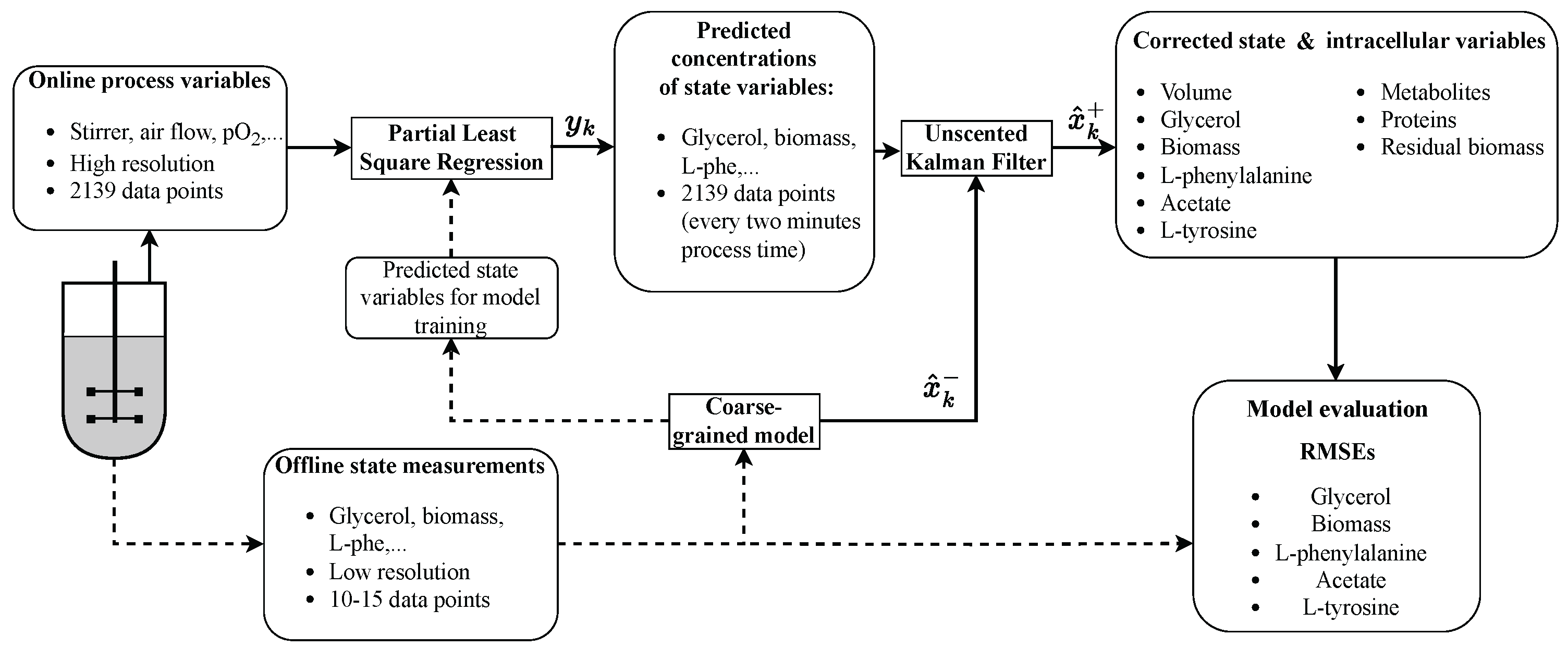
2.7. PLSR
2.8. Unscented Kalman Filter
3. Results
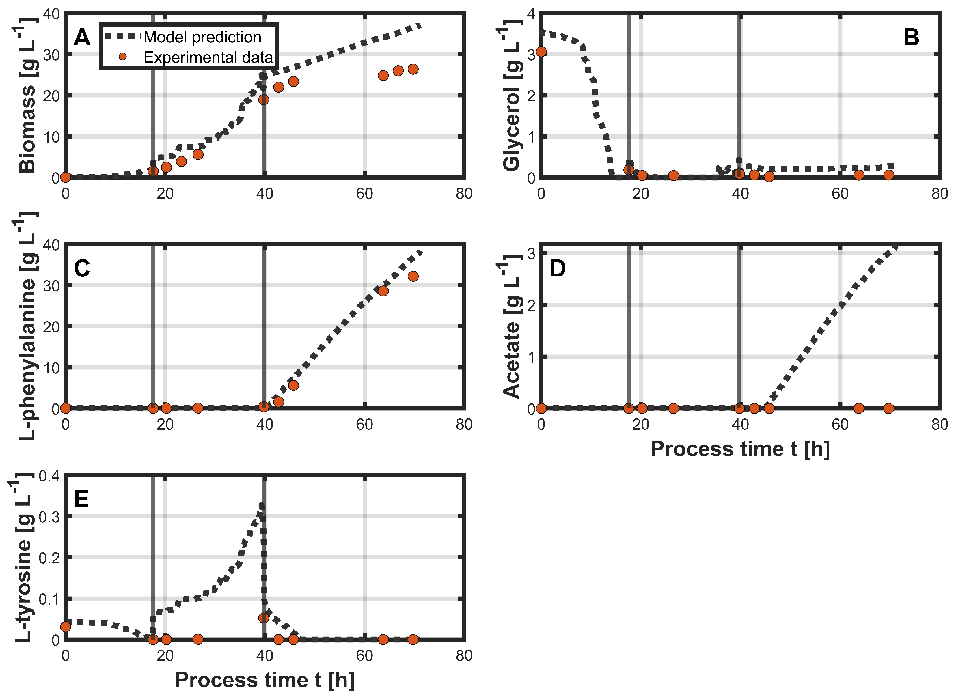
3.1. PLSR
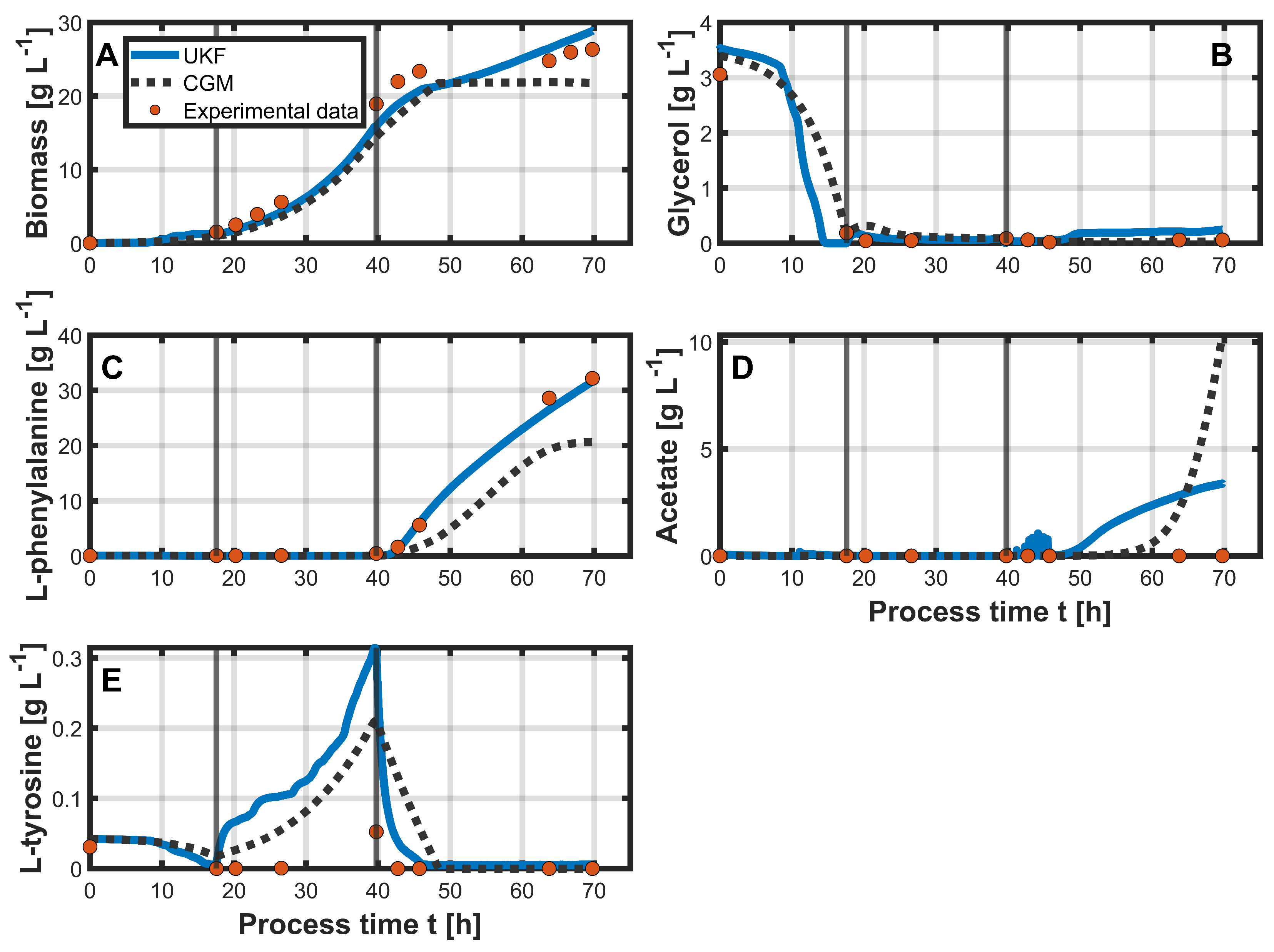
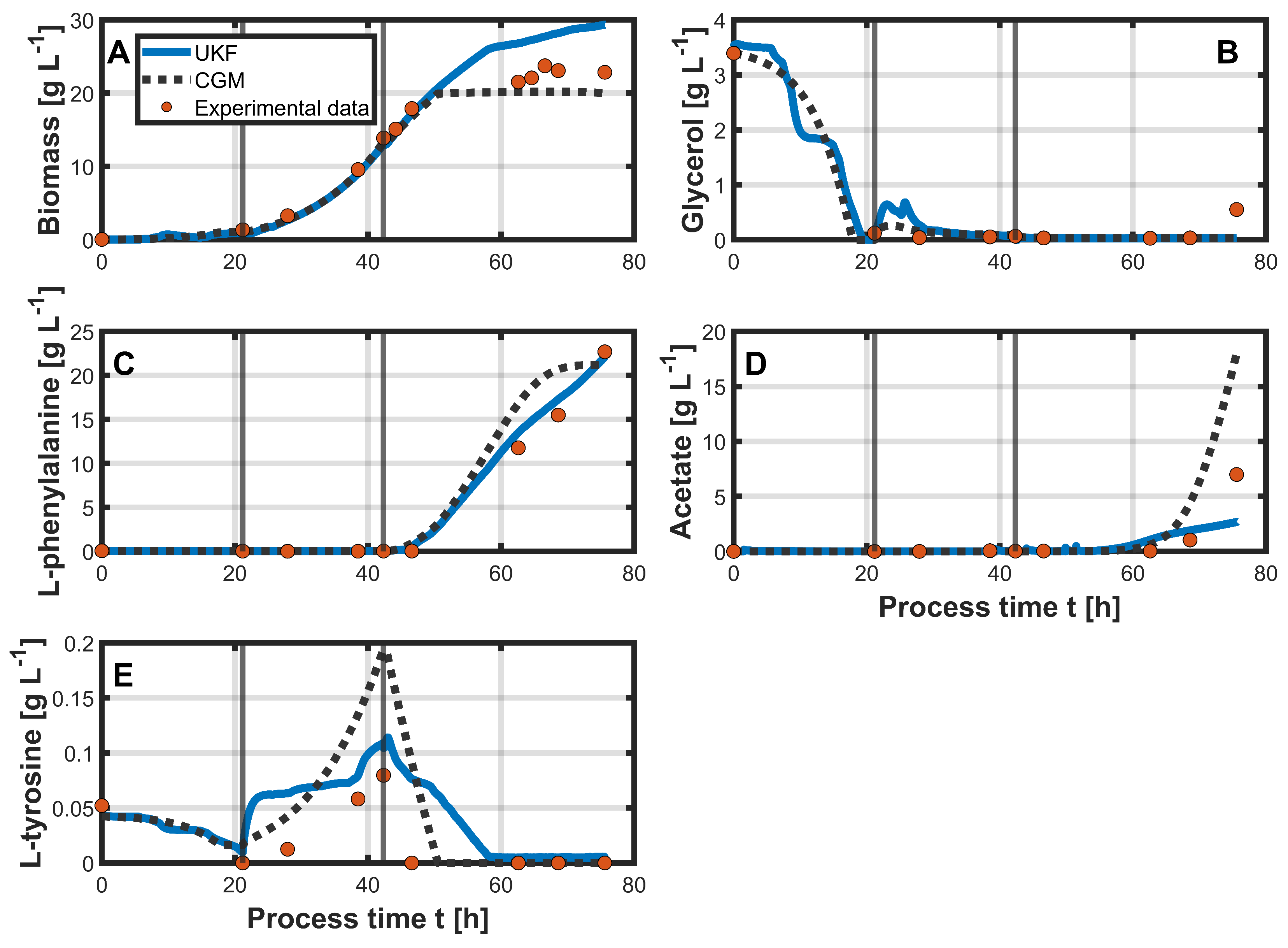
3.2. Hybrid Approach
4. Discussion
5. Conclusions
Supplementary Materials
Author Contributions
Funding
Institutional Review Board Statement
Informed Consent Statement
Data Availability Statement
Acknowledgments
Conflicts of Interest
References
- Erickson, B.; Winters, P. Perspective on opportunities in industrial biotechnology in renewable chemicals. Biotechnol. J. 2012, 7, 176–185. [Google Scholar] [CrossRef] [PubMed]
- Heins, A.L.; Hoang, M.D.; Weuster-Botz, D. Advances in automated real-time flow cytometry for monitoring of bioreactor processes. Eng. Life Sci. 2022, 22, 260–278. [Google Scholar] [CrossRef] [PubMed]
- Zhu, Y.H.; Rajalahti, T.; Linko, S. Application of neural networks to lysine production. Chem. Eng. J. Biochem. Eng. J. 1996, 62, 207–214. [Google Scholar] [CrossRef]
- Zorzetto, L.; Wilson, J.A. Monitoring bioprocesses using hybrid models and an extended Kalman filter. Comput. Chem. Eng. 1996, 20, S689–S694. [Google Scholar] [CrossRef]
- Dubach, A.C.; Märkl, H. Application of an extended kalman filter method for monitoring high density cultivation of Escherichia coli. J. Ferment. Bioeng. 1992, 73, 396–402. [Google Scholar] [CrossRef]
- Skibsted, E.; Lindemann, C.; Roca, C.; Olsson, L. On-line bioprocess monitoring with a multi-wavelength fluorescence sensor using multivariate calibration. J. Biotech. 2001, 88, 47–57. [Google Scholar] [CrossRef]
- Brunner, V.; Siegl, M.; Geier, D.; Becker, T. Challenges in the Development of Soft Sensors for Bioprocesses: A Critical Review. Front. Bioeng. Biotechnol. 2021, 9, 722202. [Google Scholar] [CrossRef]
- Kano, M.; Fujiwara, K. Virtual Sensing Technology in Process Industries: Trends and Challenges Revealed by Recent Industrial Applications. J. Chem. Eng. Jpn. 2013, 46, 1–17. [Google Scholar] [CrossRef]
- Mowbray, M.; Savage, T.; Wu, C.; Song, Z.; Cho, B.A.; Del Rio-Chanona, E.A.; Zhang, D. Machine learning for biochemical engineering: A review. Biochem. Eng. J. 2021, 172, 108054. [Google Scholar] [CrossRef]
- Vojinović, V.; Cabral, J.; Fonseca, L.P. Real-time bioprocess monitoring. Sens. Actuators B Chem. 2006, 114, 1083–1091. [Google Scholar] [CrossRef]
- Jenzsch, M.; Simutis, R.; Eisbrenner, G.; Stückrath, I.; Lübbert, A. Estimation of biomass concentrations in fermentation processes for recombinant protein production. Bioprocess Biosyst. Eng. 2006, 29, 19–27. [Google Scholar] [CrossRef] [PubMed]
- Odman, P.; Johansen, C.L.; Olsson, L.; Gernaey, K.V.; Lantz, A.E. On-line estimation of biomass, glucose and ethanol in Saccharomyces cerevisiae cultivations using in-situ multi-wavelength fluorescence and software sensors. J. Biotech. 2009, 144, 102–112. [Google Scholar] [CrossRef] [PubMed]
- Krämer, D.; King, R. A hybrid approach for bioprocess state estimation using NIR spectroscopy and a sigma-point Kalman filter. J. Process Contr. 2019, 82, 91–104. [Google Scholar] [CrossRef]
- Berg, C.; Ihling, N.; Finger, M.; Paquet-Durand, O.; Hitzmann, B.; Büchs, J. Online 2D Fluorescence Monitoring in Microtiter Plates Allows Prediction of Cultivation Parameters and Considerable Reduction in Sampling Efforts for Parallel Cultivations of Hansenula polymorpha. Bioengineering 2022, 9, 438. [Google Scholar] [CrossRef] [PubMed]
- Golabgir, A.; Herwig, C. Combining Mechanistic Modeling and Raman Spectroscopy for Real–Time Monitoring of Fed–Batch Penicillin Production. Chem. Ing. Tech. 2016, 88, 764–776. [Google Scholar] [CrossRef]
- Zhu, X.; Rehman, K.U.; Wang, B.; Shahzad, M. Modern Soft-Sensing Modeling Methods for Fermentation Processes. Sensors 2020, 20, 1771. [Google Scholar] [CrossRef]
- Yousefi-Darani, A.; Paquet-Durand, O.; Hitzmann, B. The Kalman Filter for the Supervision of Cultivation Processes. Adv. Biochem. Eng./Biotechnol. 2021, 177, 95–125. [Google Scholar]
- Solle, D.; Hitzmann, B.; Herwig, C.; Pereira Remelhe, M.; Ulonska, S.; Wuerth, L.; Prata, A.; Steckenreiter, T. Between the Poles of Data–Driven and Mechanistic Modeling for Process Operation. Chem. Ing. Tech. 2017, 89, 542–561. [Google Scholar] [CrossRef]
- Molenaar, D.; van Berlo, R.; de Ridder, D.; Teusink, B. Shifts in growth strategies reflect tradeoffs in cellular economics. Mol. Syst. Biol. 2009, 5, 323. [Google Scholar] [CrossRef]
- Doan, D.T.; Hoang, M.D.; Heins, A.L.; Kremling, A. Applications of Coarse-Grained Models in Metabolic Engineering. Front. Mol. Biosci. 2022, 9, 806213. [Google Scholar] [CrossRef]
- Serbanescu, D.; Ojkic, N.; Banerjee, S. Cellular resource allocation strategies for cell size and shape control in bacteria. FEBS J. 2022, 289, 7891–7906. [Google Scholar] [CrossRef] [PubMed]
- Scott, M.; Hwa, T. Shaping bacterial gene expression by physiological and proteome allocation constraints. Nat. Rev. Microbiol. 2023, 21, 327–342. [Google Scholar] [CrossRef] [PubMed]
- Basan, M.; Hui, S.; Okano, H.; Zhang, Z.; Shen, Y.; Williamson, J.R.; Hwa, T. Overflow metabolism in Escherichia coli results from efficient proteome allocation. Nature 2015, 528, 99–104. [Google Scholar] [CrossRef]
- Weiner, M.; Tröndle, J.; Albermann, C.; Sprenger, G.A.; Weuster-Botz, D. Carbon storage in recombinant Escherichia coli during growth on glycerol and lactic acid. Biotechnol. Bioeng. 2014, 111, 2508–2519. [Google Scholar] [CrossRef]
- Hoang, M.D.; Polte, I.; Frantzmann, L.; von den Eichen, N.; Heins, A.L.; Weuster-Botz, D. Impact of mixing insufficiencies on L-phenylalanine production with an Escherichia coli reporter strain in a novel two-compartment bioreactor. Microb. Cell Fact. 2023, 22, 153. [Google Scholar] [CrossRef] [PubMed]
- de Jong, S. SIMPLS: An alternative approach to partial least squares regression. Chemom. Intell. Lab. Syst. 1993, 18, 251–263. [Google Scholar] [CrossRef]
- Simon, D. Optimal State Estimation; John Wiley & Sons, Inc.: Hoboken, NJ, USA, 2006; ISBN 9780470045343. [Google Scholar]
- Tuveri, A.; Pérez-García, F.; Lira-Parada, P.A.; Imsland, L.; Bar, N. Sensor fusion based on Extended and Unscented Kalman Filter for bioprocess monitoring. J. Process Contr. 2021, 106, 195–207. [Google Scholar] [CrossRef]
- Narayanan, H.; Behle, L.; Luna, M.F.; Sokolov, M.; Guillén-Gosálbez, G.; Morbidelli, M.; Butté, A. Hybrid-EKF: Hybrid model coupled with extended Kalman filter for real-time monitoring and control of mammalian cell culture. Biotechnol. Bioeng. 2020, 117, 2703–2714. [Google Scholar] [CrossRef]
- Kozmai, A.; Porozhnyy, M.; Gil, V.; Dammak, L. Phenylalanine Losses in Neutralization Dialysis: Modeling and Experiment. Membranes 2023, 13, 506. [Google Scholar] [CrossRef]
- Siegl, M.; Kämpf, M.; Geier, D.; Andreeßen, B.; Max, S.; Zavrel, M.; Becker, T. Generalizability of Soft Sensors for Bioprocesses through Similarity Analysis and Phase-Dependent Recalibration. Sensors 2023, 23, 2178. [Google Scholar] [CrossRef]
- Routledge, S.J. Beyond de-foaming: The effects of antifoams on bioprocess productivity. Comput. Struct. Biotechnol. J. 2012, 3, e201210014. [Google Scholar] [CrossRef] [PubMed]
- Zavala-Ortiz, D.A.; Denner, A.; Aguilar-Uscanga, M.G.; Marc, A.; Ebel, B.; Guedon, E. Comparison of partial least square, artificial neural network, and support vector regressions for real-time monitoring of CHO cell culture processes using in situ near-infrared spectroscopy. Biotechnol. Bioeng. 2022, 119, 535–549. [Google Scholar] [CrossRef] [PubMed]
- Lee, H.L.; Boccazzi, P.; Gorret, N.; Ram, R.J.; Sinskey, A.J. In situ bioprocess monitoring of Escherichia coli bioreactions using Raman spectroscopy. Vib. Spectrosc. 2004, 35, 131–137. [Google Scholar] [CrossRef]
- Kornmann, H.; Rhiel, M.; Cannizzaro, C.; Marison, I.; von Stockar, U. Methodology for real-time, multianalyte monitoring of fermentations using an in-situ mid-infrared sensor. Biotechnol. Bioeng. 2003, 82, 702–709. [Google Scholar] [CrossRef]
- Broger, T.; Odermatt, R.P.; Huber, P.; Sonnleitner, B. Real-time on-line flow cytometry for bioprocess monitoring. J. Biotech. 2011, 154, 240–247. [Google Scholar] [CrossRef]
- Delvigne, F.; Boxus, M.; Ingels, S.; Thonart, P. Bioreactor mixing efficiency modulates the activity of a prpoS::GFP reporter gene in E. coli. Microb. Cell fact. 2009, 8, 15. [Google Scholar] [CrossRef] [PubMed]
- Urrea, C.; Agramonte, R. Kalman Filter: Historical Overview and Review of Its Use in Robotics 60 Years after Its Creation. J. Sens. 2021, 2021, 9674015. [Google Scholar] [CrossRef]
- Krämer, D.; King, R. On-line monitoring of substrates and biomass using near-infrared spectroscopy and model-based state estimation for enzyme production by S. cerevisiae. IFAC-PapersOnLine 2016, 49, 609–614. [Google Scholar] [CrossRef]
- Zheng, B.; Fu, P.; Li, B.; Yuan, X. A Robust Adaptive Unscented Kalman Filter for Nonlinear Estimation with Uncertain Noise Covariance. Sensors 2018, 18, 808. [Google Scholar] [CrossRef]
- Dewasme, L.; Goffaux, G.; Hantson, A.L.; Wouwer, A.V. Experimental validation of an Extended Kalman Filter estimating acetate concentration in E. coli cultures. J. Process Contr. 2013, 23, 148–157. [Google Scholar] [CrossRef]
- Marafioti, G.; Tebbani, S.; Beauvois, D.; Becerra, G.; Isambert, A.; Hovd, M. Unscented Kalman Filter state and parameter estimation in a photobioreactor for microalgae production. IFAC Proc. Vol. 2009, 42, 804–809. [Google Scholar] [CrossRef]
- Kemmer, A.; Fischer, N.; Wilms, T.; Cai, L.; Groß, S.; King, R.; Neubauer, P.; Cruz Bournazou, M.N. Nonlinear state estimation as tool for online monitoring and adaptive feed in high throughput cultivations. Biotechnol. Bioeng. 2023, 120, 3261–3275. [Google Scholar] [CrossRef] [PubMed]
- Sprenger, G.A. From scratch to value: Engineering Escherichia coli wild type cells to the production of L-phenylalanine and other fine chemicals derived from chorismate. Appl. Microbiol. Biotechnol. 2007, 75, 739–749. [Google Scholar] [CrossRef]
- Snoeck, S.; Guidi, C.; de Mey, M. “Metabolic burden” explained: Stress symptoms and its related responses induced by (over)expression of (heterologous) proteins in Escherichia coli. Microb. Cell Fact. 2024, 23, 96. [Google Scholar] [CrossRef]
- van Riel, N.A.W. A Template for Parameter Estimation with Matlab Optimization Toolbox; Including Dynamic Systems. Available online: www.researchgate.net/publication/269930829_A_template_for_parameter_estimation_with_Matlab_Optimization_Toolbox_including_dynamic_systems (accessed on 11 June 2025).


| State Variables | RMSE | ||
|---|---|---|---|
| Process 1 (Training) | Process 2 (Prediction) | Process 3 (Prediction) | |
| Biomass [g L−1] | 0.95 | 5.59 | 5.8 |
| Glycerol [g L−1] | 0.12 | 0.24 | 0.22 |
| L-phenylalanine [g L−1] | 0.43 | 1.81 | 0.99 |
| Acetate [g L−1] | 0.3 | 1.29 | 1.61 |
| L-tyrosine [g L−1] | 0.02 | 0.09 | 0.04 |
| State Variables | RMSE | |||
|---|---|---|---|---|
| Process 2 | Process 3 | |||
| CGM | UKF | CGM | UKF | |
| Biomass [g L−1] | 3.15 | 1.94 | 1.74 | 3.43 |
| Glycerol [g L−1] | 0.15 | 0.19 | 0.18 | 0.2 |
| L-phenylalanine [g L−1] | 5.14 | 0.76 | 2.48 | 0.87 |
| Acetate [g L−1] | 3.51 | 1.47 | 3.84 | 1.51 |
| L-tyrosine [g L−1] | 0.07 | 0.1 | 0.06 | 0.03 |
Disclaimer/Publisher’s Note: The statements, opinions and data contained in all publications are solely those of the individual author(s) and contributor(s) and not of MDPI and/or the editor(s). MDPI and/or the editor(s) disclaim responsibility for any injury to people or property resulting from any ideas, methods, instructions or products referred to in the content. |
© 2025 by the authors. Licensee MDPI, Basel, Switzerland. This article is an open access article distributed under the terms and conditions of the Creative Commons Attribution (CC BY) license (https://creativecommons.org/licenses/by/4.0/).
Share and Cite
Hermann, L.; Kremling, A. A Hybrid Soft Sensor Approach Combining Partial Least-Squares Regression and an Unscented Kalman Filter for State Estimation in Bioprocesses. Bioengineering 2025, 12, 654. https://doi.org/10.3390/bioengineering12060654
Hermann L, Kremling A. A Hybrid Soft Sensor Approach Combining Partial Least-Squares Regression and an Unscented Kalman Filter for State Estimation in Bioprocesses. Bioengineering. 2025; 12(6):654. https://doi.org/10.3390/bioengineering12060654
Chicago/Turabian StyleHermann, Lucas, and Andreas Kremling. 2025. "A Hybrid Soft Sensor Approach Combining Partial Least-Squares Regression and an Unscented Kalman Filter for State Estimation in Bioprocesses" Bioengineering 12, no. 6: 654. https://doi.org/10.3390/bioengineering12060654
APA StyleHermann, L., & Kremling, A. (2025). A Hybrid Soft Sensor Approach Combining Partial Least-Squares Regression and an Unscented Kalman Filter for State Estimation in Bioprocesses. Bioengineering, 12(6), 654. https://doi.org/10.3390/bioengineering12060654