Author Contributions
Conceptualization, M.R.A., Z.H.L., H.R., R.H., S.M.M.R.S., Y.-I.C. and M.S.A.; methodology, M.R.A., M.I.H.S., Z.H.L., H.R., Y.-I.C. and M.S.A.; software, M.A.K., A.S.U.K.P. and M.I.H.S.; formal analysis, Y.-I.C., S.M.M.R.S., R.H., M.R.A., H.R., M.A.K. and M.S.A.; investigation, Z.H.L., M.R.A., M.A.K., A.S.U.K.P. and S.M.M.R.S.; data curation, M.I.H.S., A.S.U.K.P. and H.R.; writing—original draft preparation, M.R.A., Z.H.L., M.I.H.S., H.R., M.A.K. and A.S.U.K.P.; writing—review and editing, M.R.A., Z.H.L., M.I.H.S., H.R., M.A.K., S.M.M.R.S., R.H. and M.S.A.; visualization, R.H., M.I.H.S., M.A.K., S.M.M.R.S. and M.R.A.; validation, M.A.K., R.H., A.S.U.K.P. and M.S.A.; supervision, M.S.A. and Y.-I.C. and M.S.A.; project administration, Y.-I.C. and M.S.A.; funding acquisition, Y.-I.C. All authors have read and agreed to the published version of the manuscript.
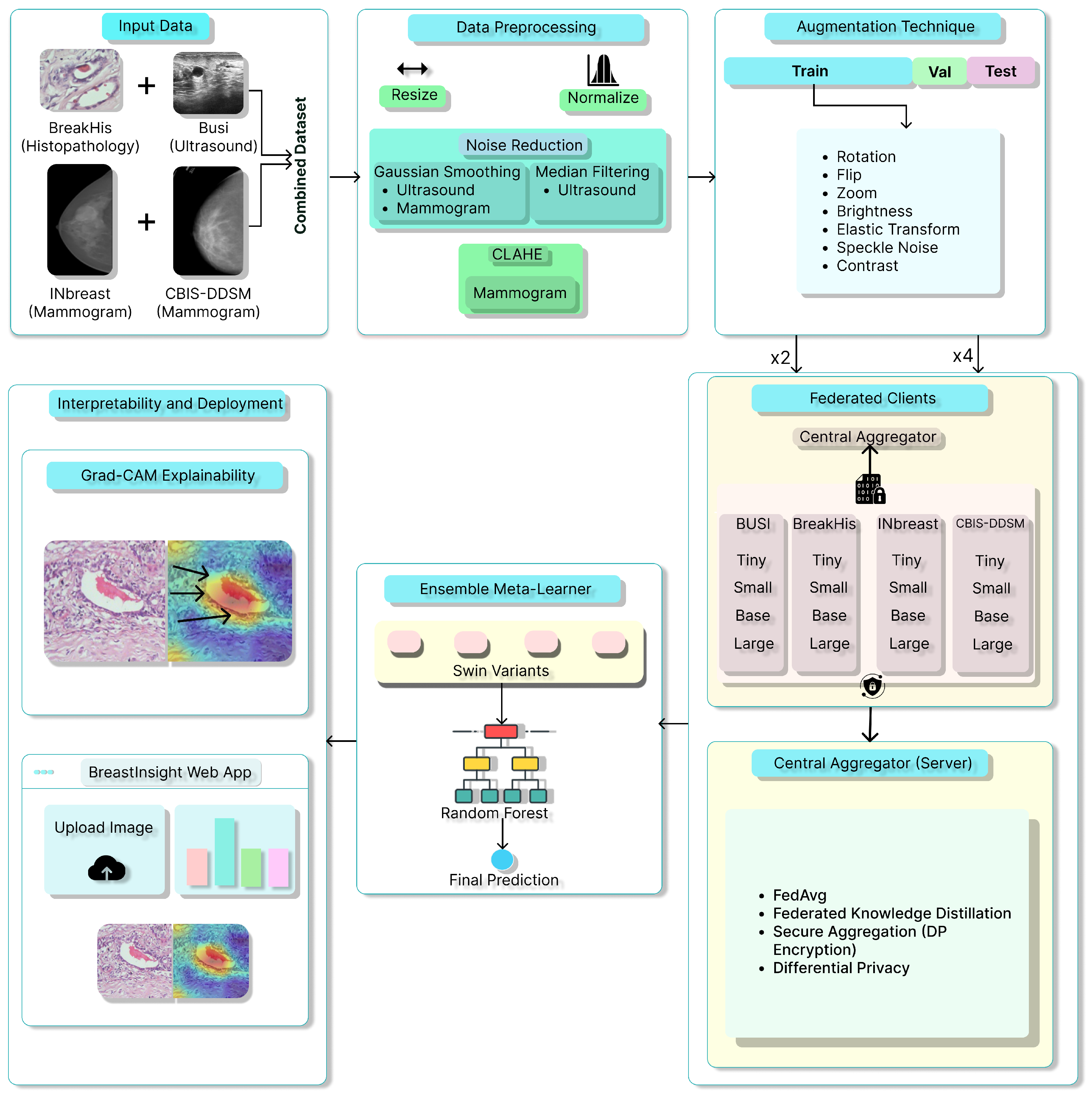
Figure 1.
Overview of the proposed BreastSwimFedNetX for robust breast cancer classification. Black arrows in Grad-CAM Explainability subfigure indicate the model’s attention focus.
Figure 1.
Overview of the proposed BreastSwimFedNetX for robust breast cancer classification. Black arrows in Grad-CAM Explainability subfigure indicate the model’s attention focus.
Figure 2.
Representative samples from the BreakHis dataset showing benign and malignant breast tissue histopathological images across different magnifications (40×, 100×, 200×, and 400×). The benign samples include Adenosis, Fibroadenoma, Phyllodes Tumor, and Tubular Adenoma, while the malignant samples consist of Ductal Carcinoma, Lobular Carcinoma, Mucinous Carcinoma, and Papillary Carcinoma.
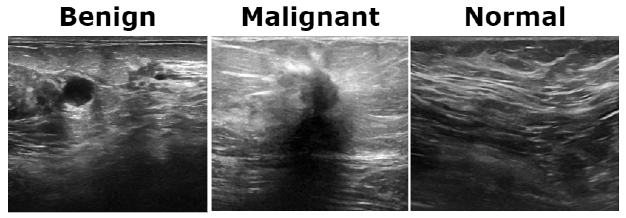
Figure 3.
Representative ultrasound images from the BUSI dataset showcasing three classes.
Figure 3.
Representative ultrasound images from the BUSI dataset showcasing three classes.
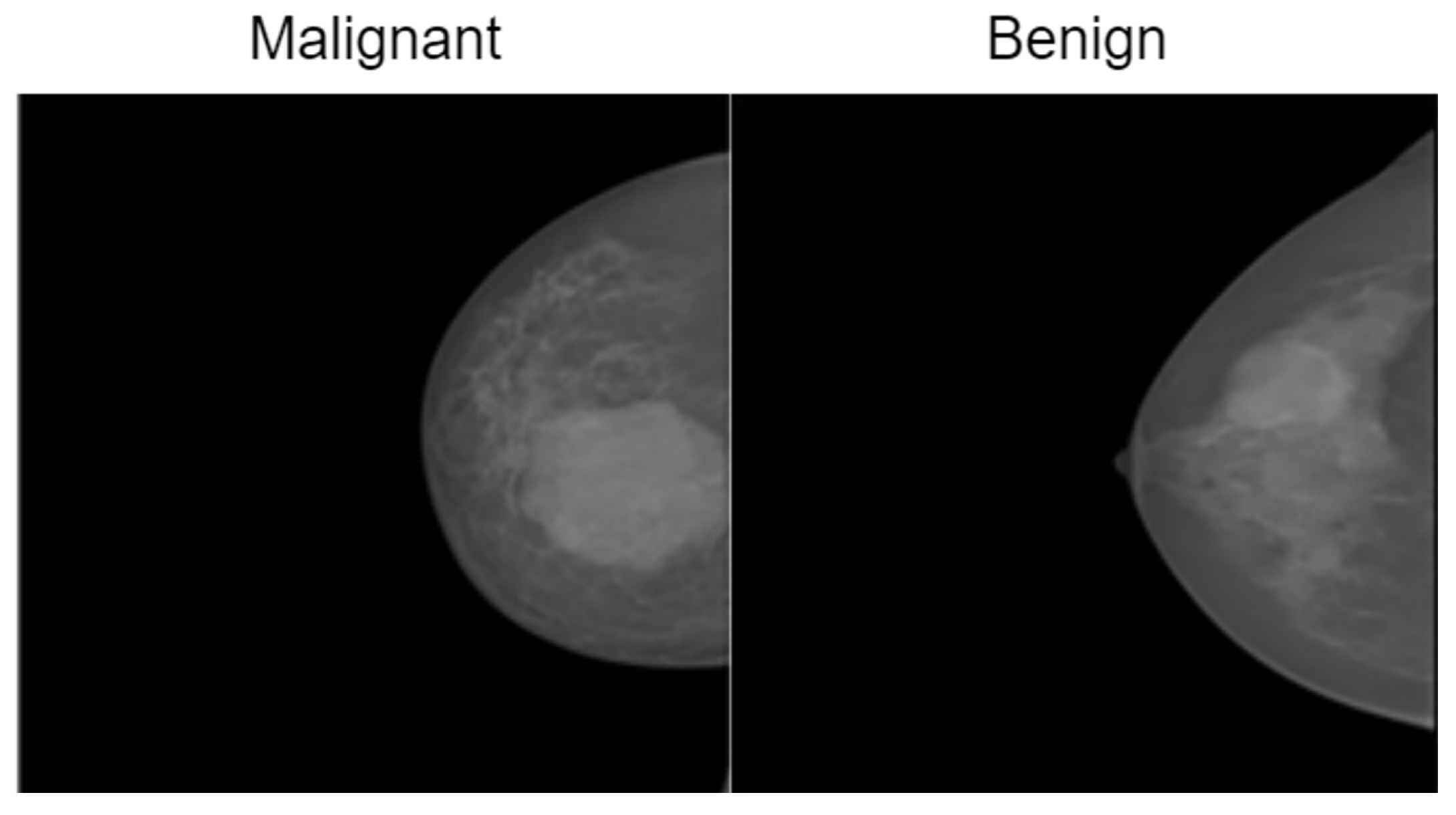
Figure 4.
Representative samples from the InBreast dataset showing malignant and normal classes.
Figure 4.
Representative samples from the InBreast dataset showing malignant and normal classes.
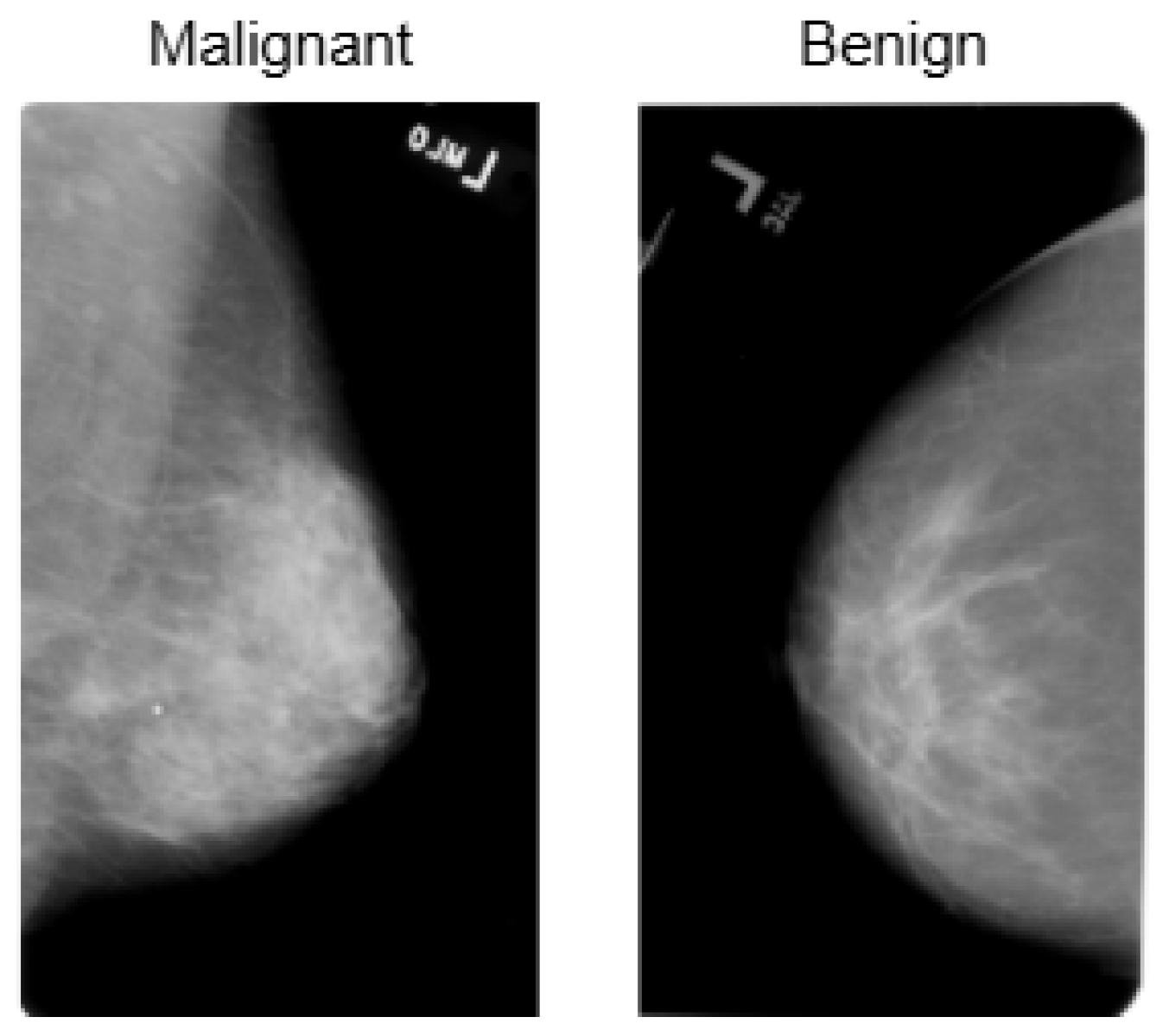
Figure 5.
Visualization of the CBIS-DDSM dataset, highlighting its structure and distribution for breast cancer classification.
Figure 5.
Visualization of the CBIS-DDSM dataset, highlighting its structure and distribution for breast cancer classification.
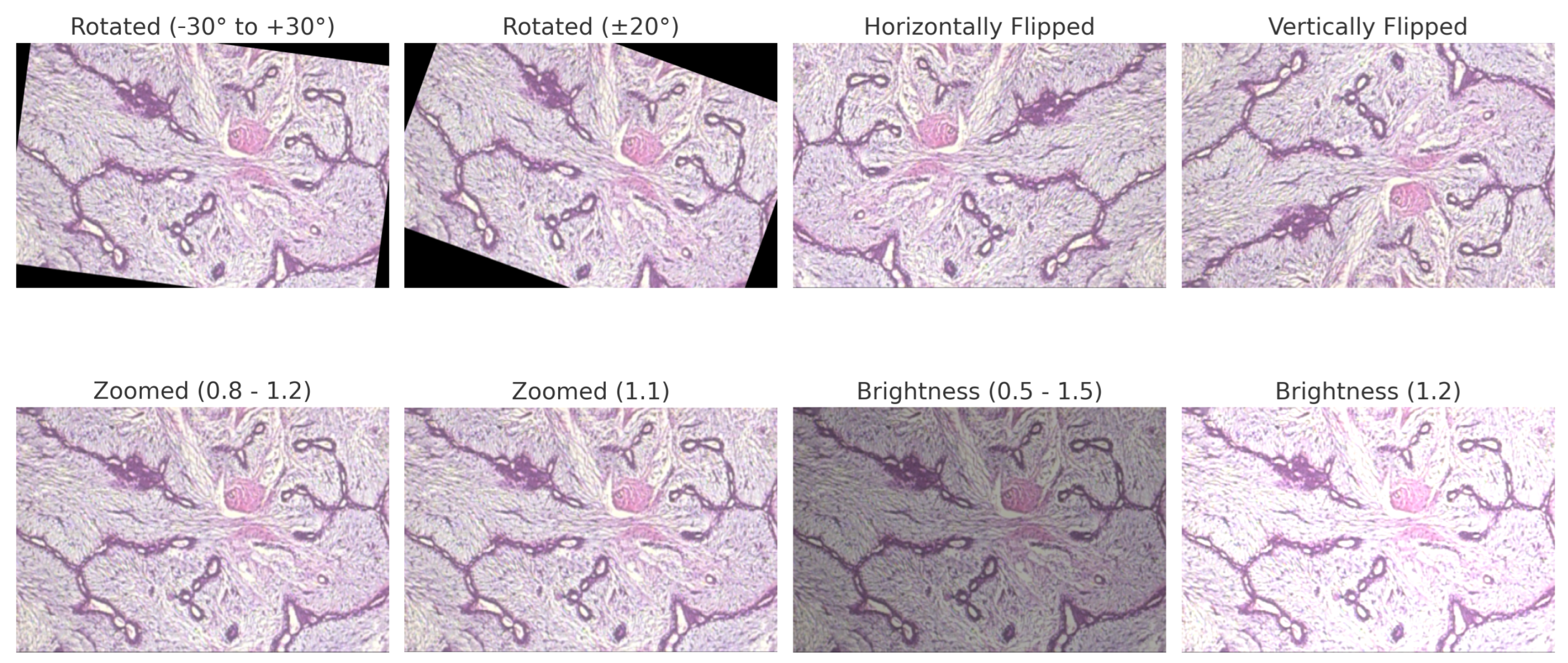
Figure 6.
BreakHis preprocessed sample with applied data augmentation techniques, including rotation, flipping, zooming, and brightness adjustment.
Figure 6.
BreakHis preprocessed sample with applied data augmentation techniques, including rotation, flipping, zooming, and brightness adjustment.
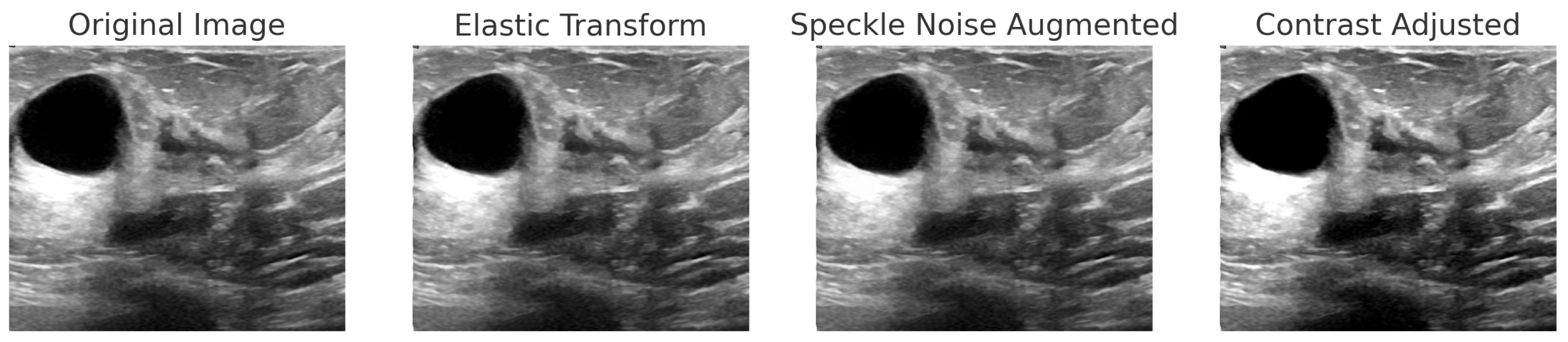
Figure 7.
Step-by-step augmentation of a BUSI dataset sample. The original ultrasound image undergoes three transformations: (1) Elastic Transform to introduce slight deformations; (2) Speckle Noise Augmentation to simulate real-world noise variations; (3) Contrast Adjustment to enhance intensity variations.
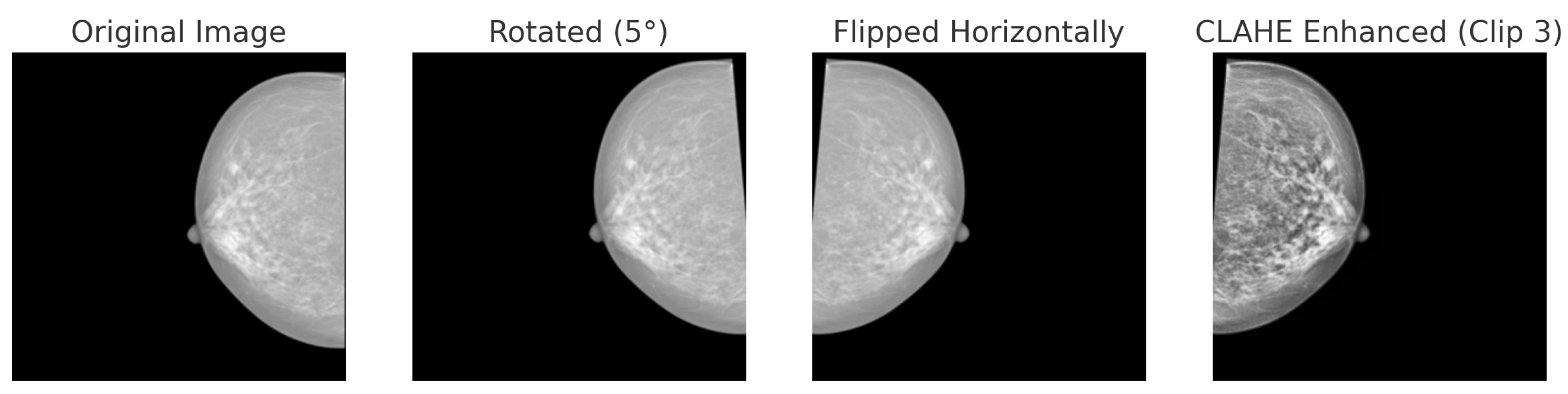
Figure 8.
Data augmentation techniques applied to a mammogram image from the INbreast dataset: original, rotated (+5°), horizontally flipped and CLAHE.
Figure 8.
Data augmentation techniques applied to a mammogram image from the INbreast dataset: original, rotated (+5°), horizontally flipped and CLAHE.
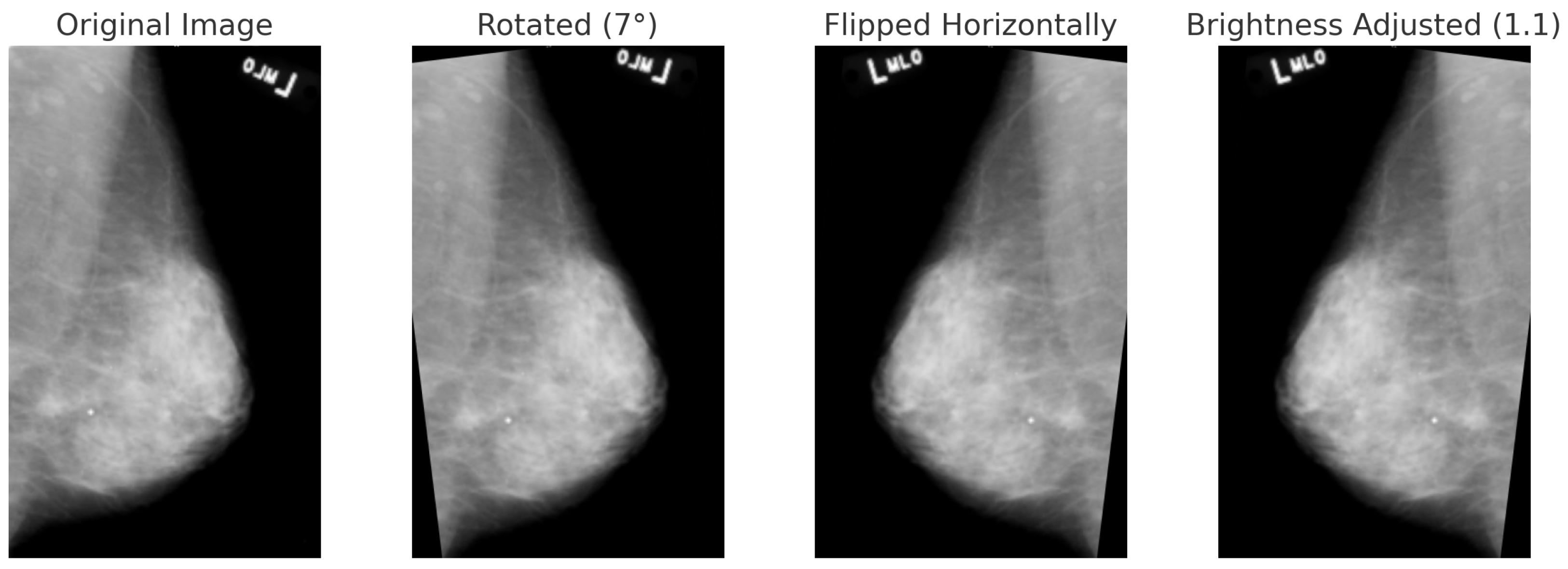
Figure 9.
Data augmentation techniques applied to a mammogram image from the CBIS-DDSM dataset: original, rotated (+7°), horizontally flipped, and brightness-adjusted.
Figure 9.
Data augmentation techniques applied to a mammogram image from the CBIS-DDSM dataset: original, rotated (+7°), horizontally flipped, and brightness-adjusted.
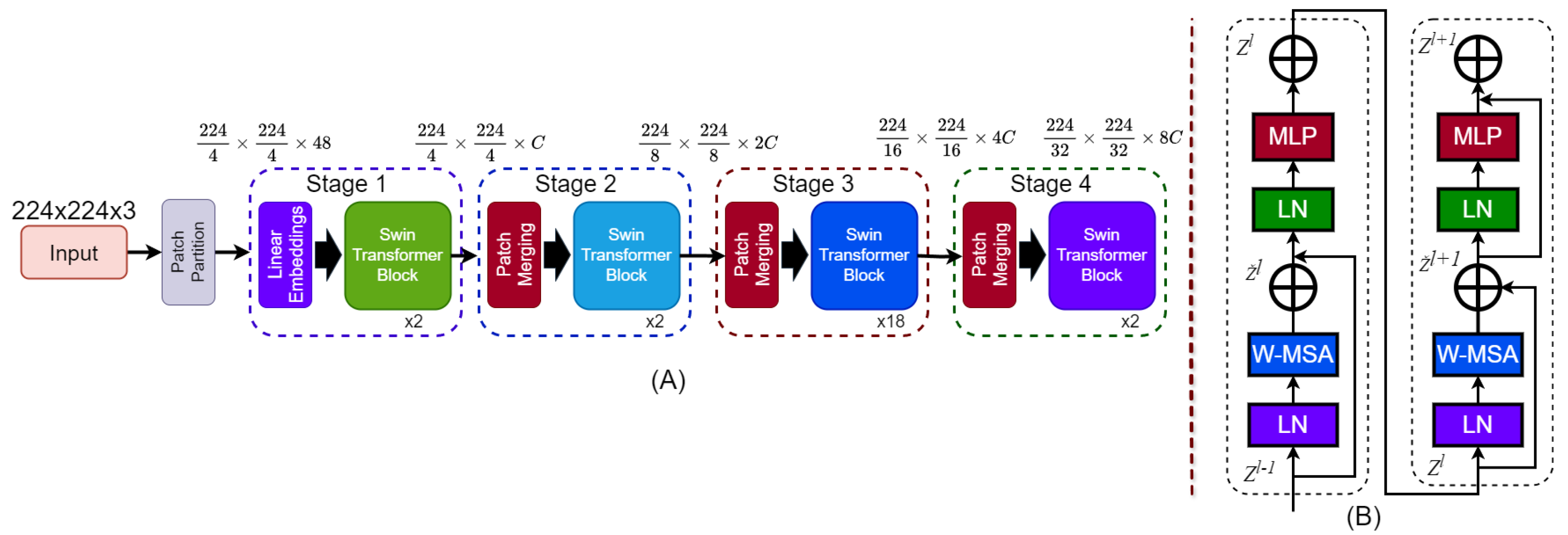
Figure 10.
Architecture of the Swin Transformer. (A) The hierarchical model structure takes a 224 × 224 × 3 input image, applies patch partitioning and linear embedding, and processes it through four stages with Swin Transformer blocks. Patch merging reduces spatial dimensions and increases feature depth across stages. (B) Structure of a Swin Transformer block showing two sub-blocks. Each includes Layer Normalization (LN), Window-based Multi-Head Self-Attention (W-MSA), and a MLP, with residual connections after W-MSA and MLP.
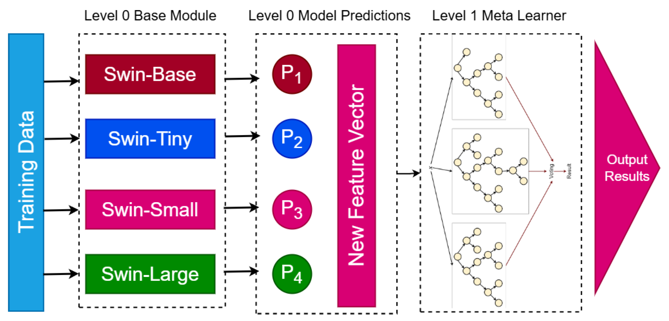
Figure 11.
Proposed BreastSwinFedNetX model architecture for multi-class classification. The Level 0 Base Module includes four Swin Transformer variants that generate predictions. These predictions form a New Feature Vector passed to the Level 1 Meta Learner, which produces the final results.
Figure 11.
Proposed BreastSwinFedNetX model architecture for multi-class classification. The Level 0 Base Module includes four Swin Transformer variants that generate predictions. These predictions form a New Feature Vector passed to the Level 1 Meta Learner, which produces the final results.
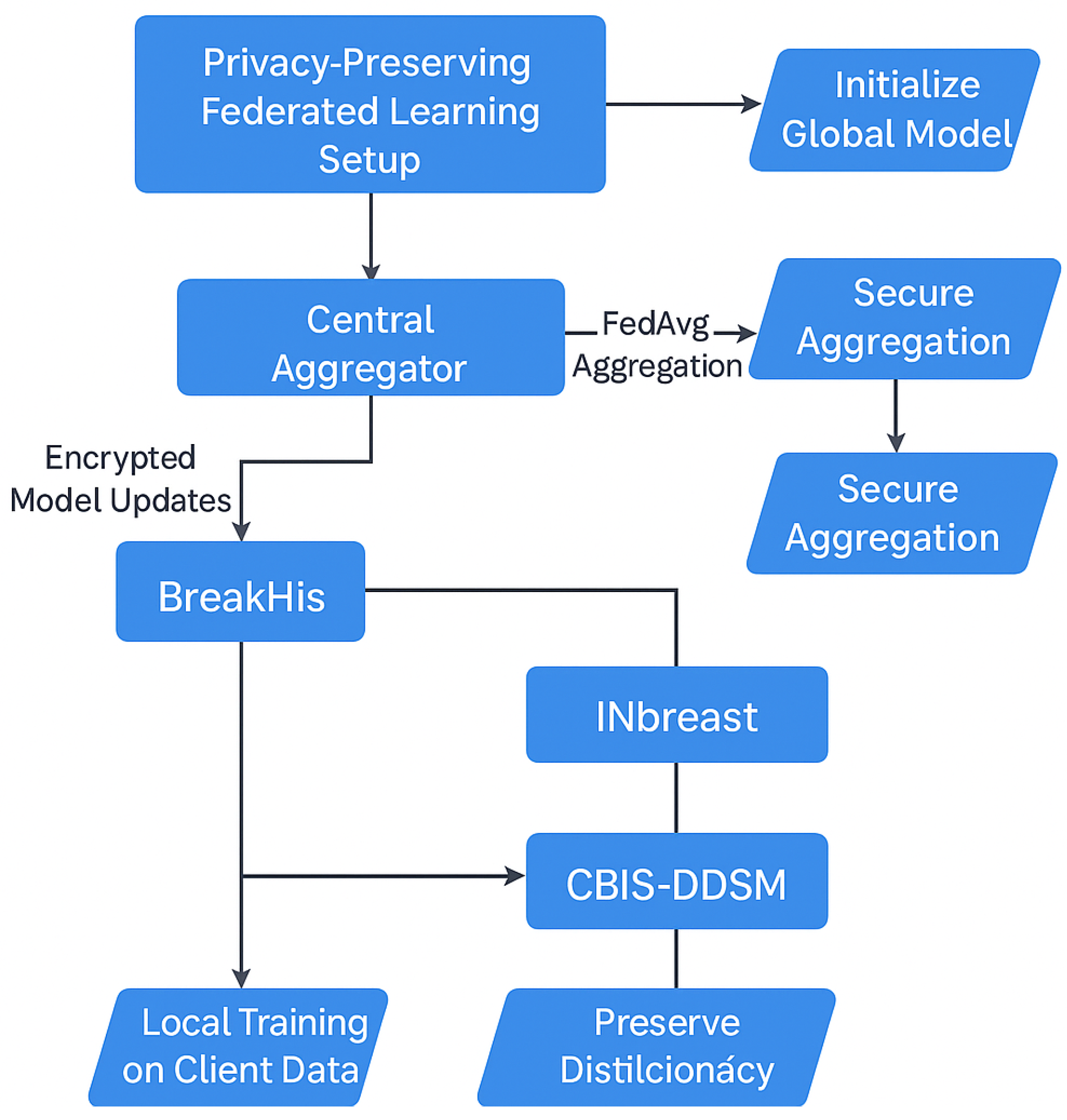
Figure 12.
FL setup in BreastSwinFedNetX.
Figure 12.
FL setup in BreastSwinFedNetX.
Figure 13.
Performance improvement of DL models across datasets before and after data augmentation.
Figure 13.
Performance improvement of DL models across datasets before and after data augmentation.
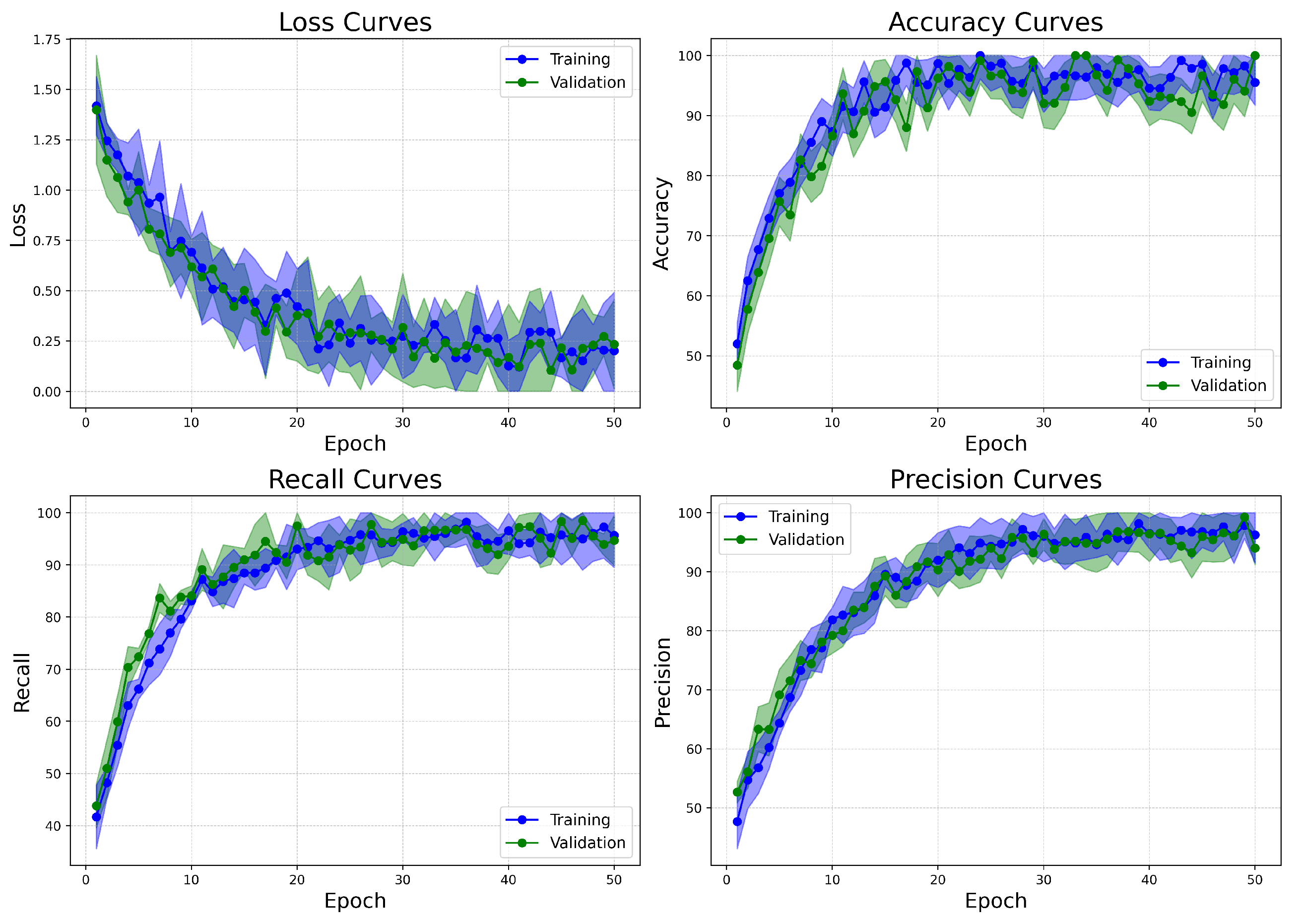
Figure 14.
Learning curves of BreastSwinFedNetX model on highest performing multiclass classification dataset.
Figure 14.
Learning curves of BreastSwinFedNetX model on highest performing multiclass classification dataset.
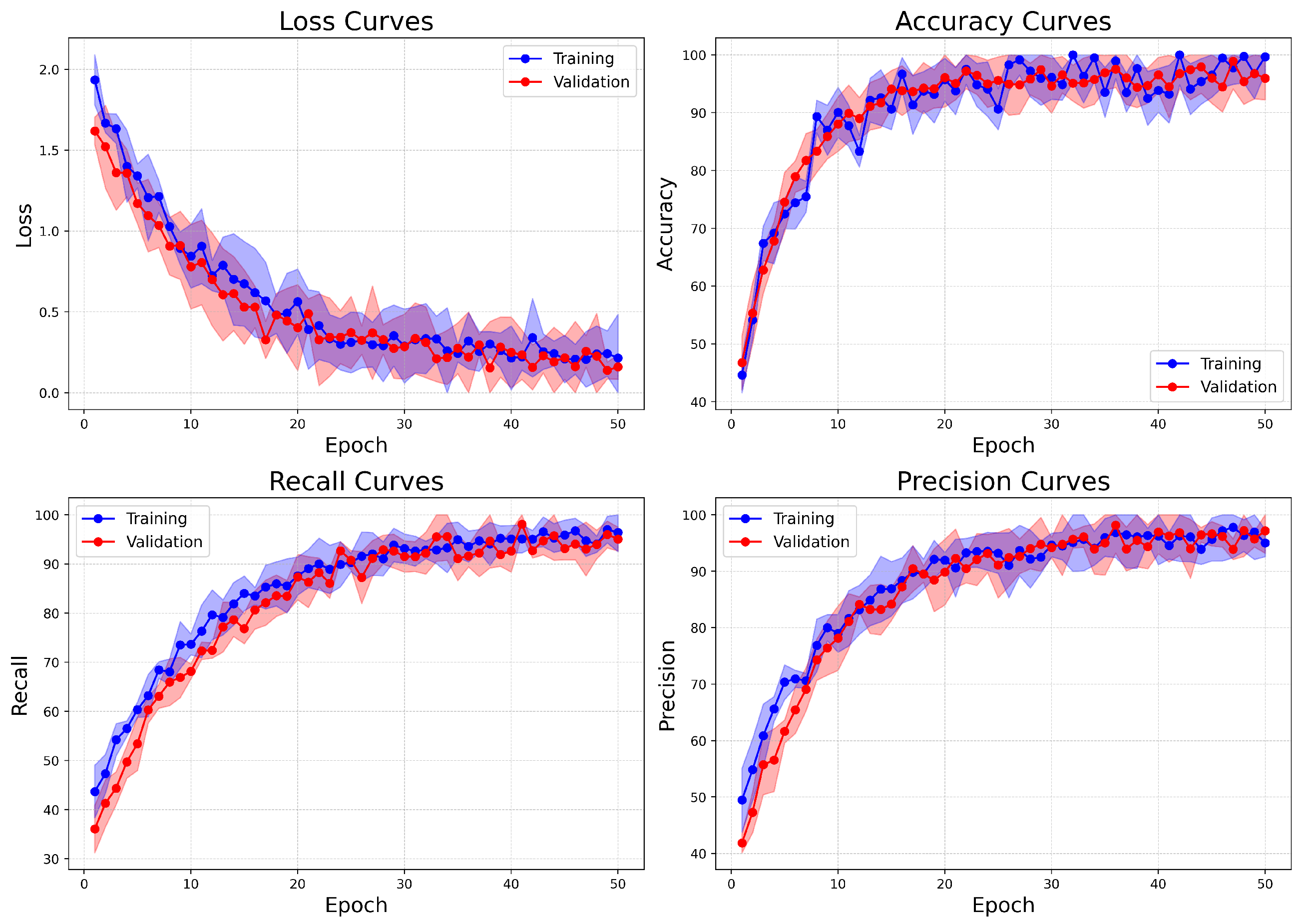
Figure 15.
Learning curves of BreastSwinFedNetX model on highest performing binary classification dataset.
Figure 15.
Learning curves of BreastSwinFedNetX model on highest performing binary classification dataset.
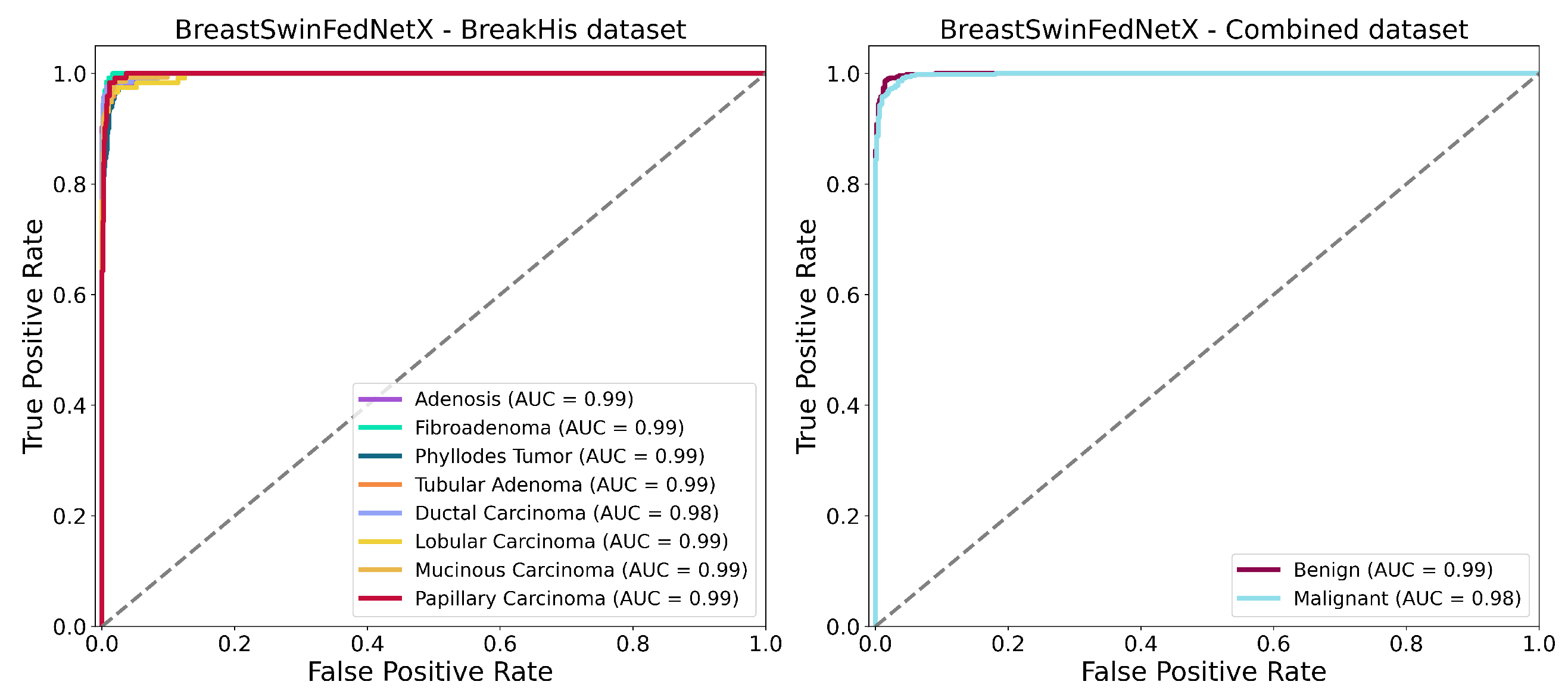
Figure 16.
ROC AUC curves of BreastSwinFedNetX model on highest performing multiclass and binary classification dataset.
Figure 16.
ROC AUC curves of BreastSwinFedNetX model on highest performing multiclass and binary classification dataset.
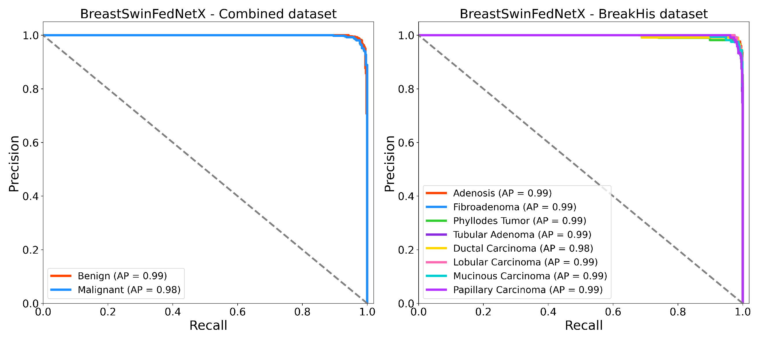
Figure 17.
Precision recall curves of BreastSwinFedNetX model on highest performing binary and multiclass classification dataset.
Figure 17.
Precision recall curves of BreastSwinFedNetX model on highest performing binary and multiclass classification dataset.
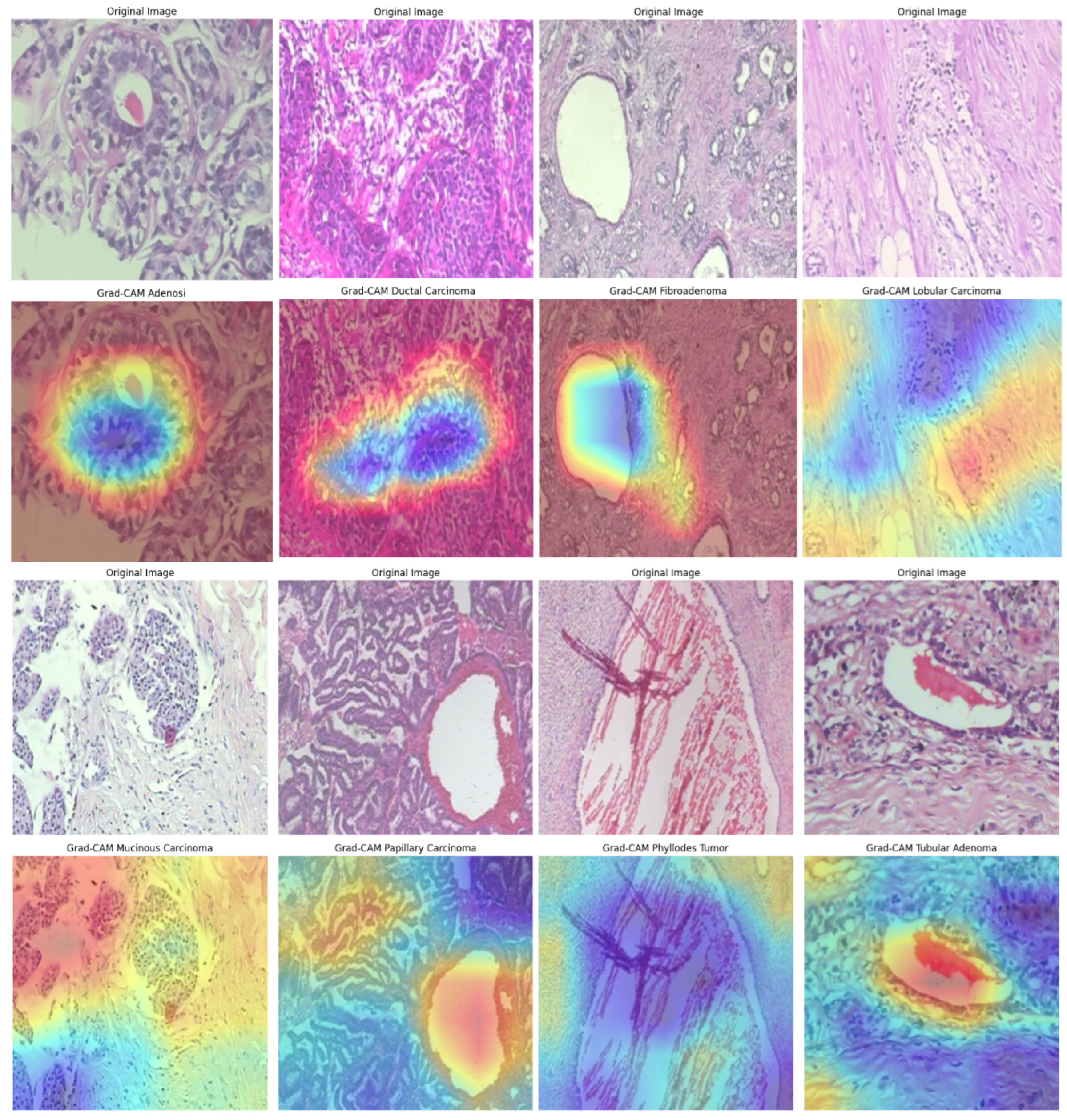
Figure 18.
Grad-CAM visualizations on the BreakHis dataset, illustrating model attention in breast cancer classification. Warmer colors (red/yellow) indicate regions of high activation, highlighting critical features used in decision-making.
Figure 18.
Grad-CAM visualizations on the BreakHis dataset, illustrating model attention in breast cancer classification. Warmer colors (red/yellow) indicate regions of high activation, highlighting critical features used in decision-making.
Figure 19.
Grad-CAM visualizations of BUSI dataset images, highlighting model focus areas for benign, malignant, and normal cases.
Figure 19.
Grad-CAM visualizations of BUSI dataset images, highlighting model focus areas for benign, malignant, and normal cases.
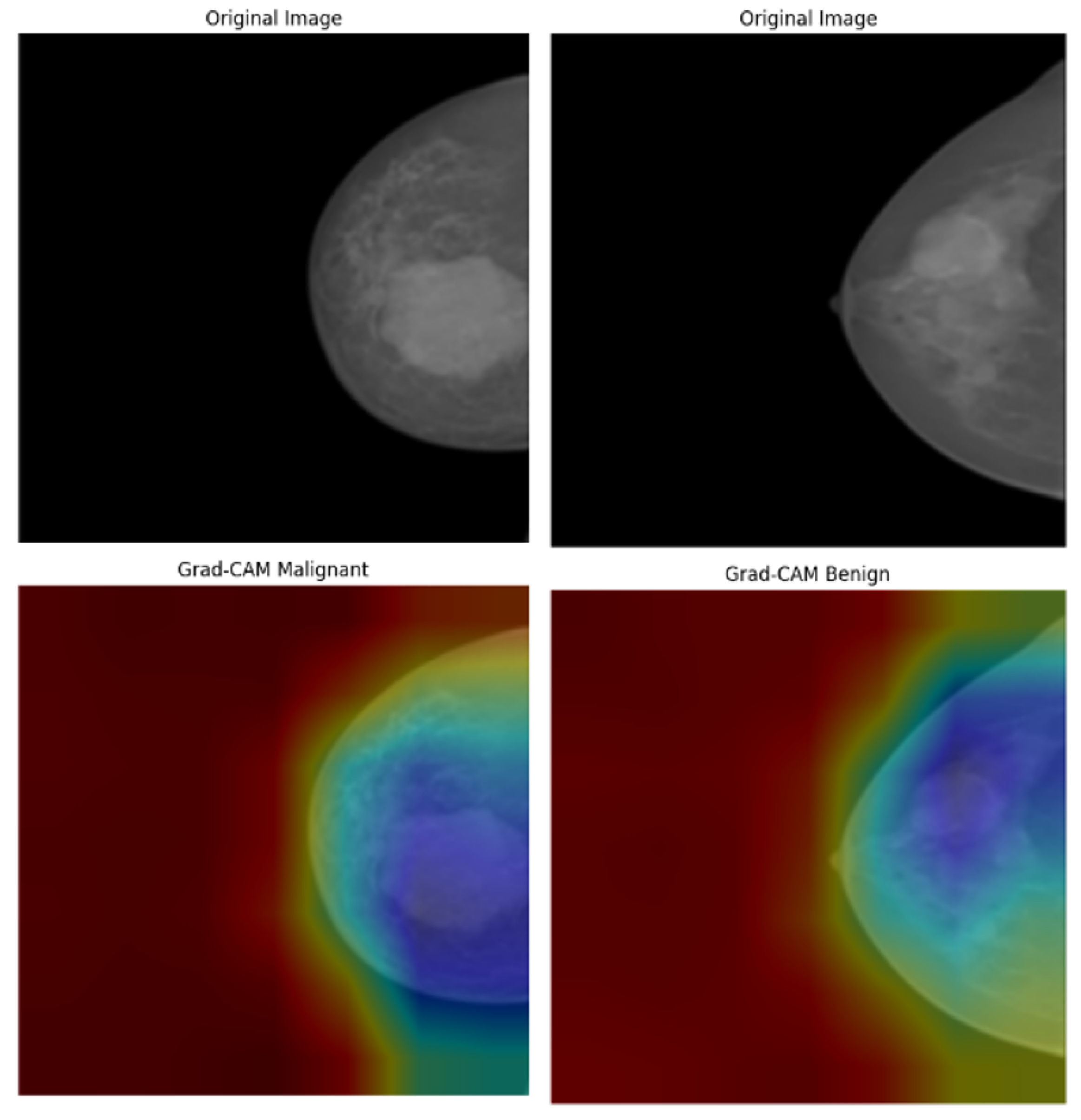
Figure 20.
Grad-CAM visualizations of INbreast mammograms highlighting model attention for malignant and benign cases.
Figure 20.
Grad-CAM visualizations of INbreast mammograms highlighting model attention for malignant and benign cases.
Figure 21.
Grad-CAM visualizations of malignant and benign cases from the CBIS-DDSM dataset.
Figure 21.
Grad-CAM visualizations of malignant and benign cases from the CBIS-DDSM dataset.
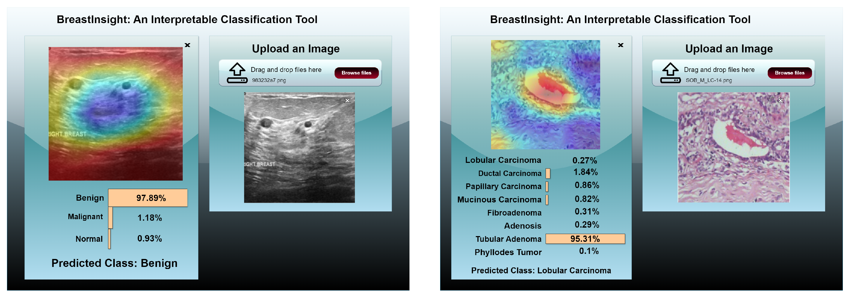
Figure 22.
BreastInsight user interface during inference. The clinicians upload an image and the global BreastSwinFedNetX model takes in the subsequently processed image. Class probabilities for each instance are displayed in the form of horizontal bars.
Figure 22.
BreastInsight user interface during inference. The clinicians upload an image and the global BreastSwinFedNetX model takes in the subsequently processed image. Class probabilities for each instance are displayed in the form of horizontal bars.
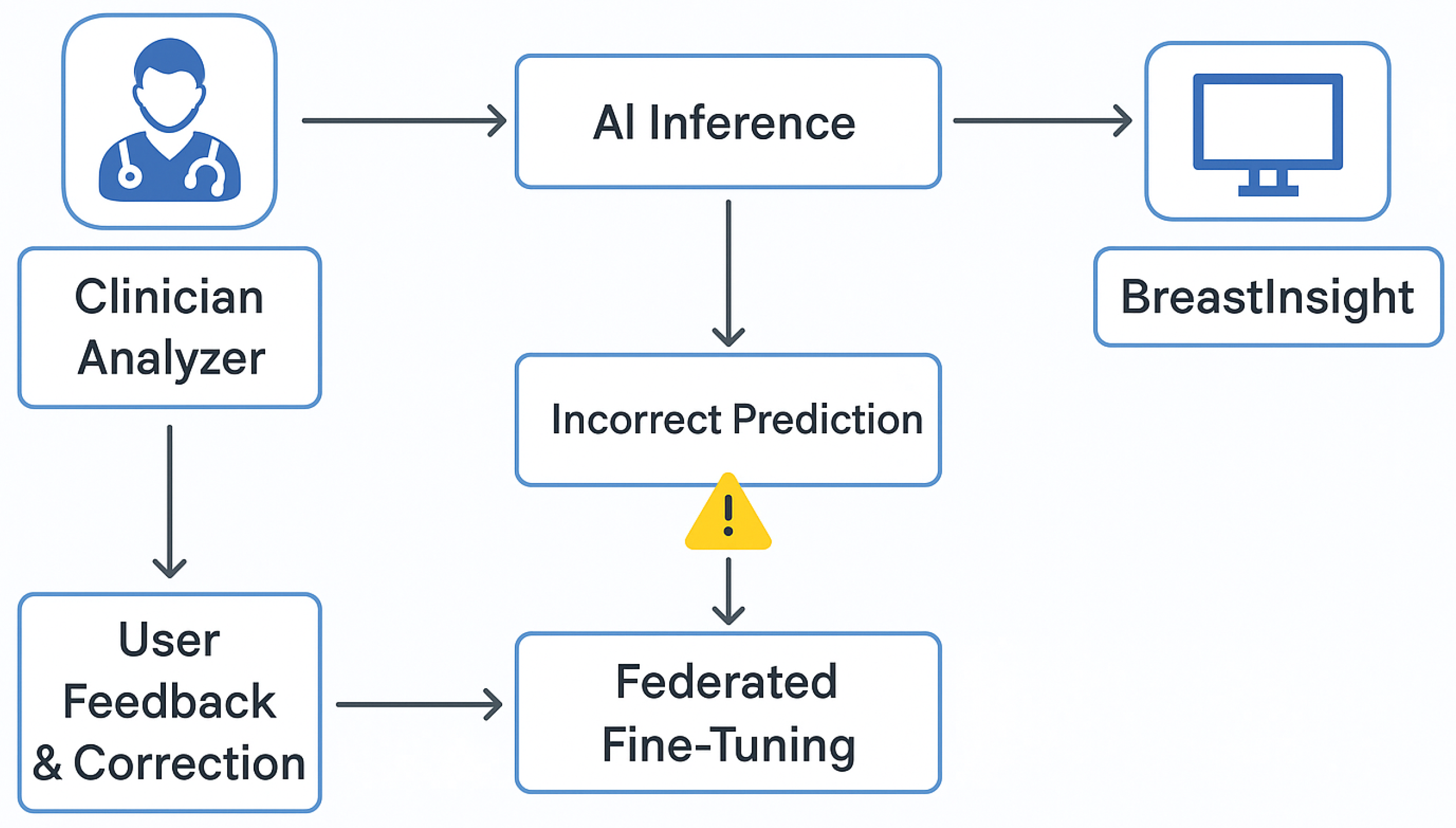
Figure 23.
Flowchart of BreastInsight’s feedback and error correction mechanism.
Figure 23.
Flowchart of BreastInsight’s feedback and error correction mechanism.
Table 1.
Class distribution of the BreakHis dataset across different magnification factors.
Table 1.
Class distribution of the BreakHis dataset across different magnification factors.
| Subtype | 40× | 100× | 200× | 400× |
|---|
| Adenosis | 114 | 113 | 111 | 106 |
| Fibroadenoma | 253 | 260 | 264 | 237 |
| Phyllodes Tumor | 109 | 121 | 108 | 115 |
| Tubular Adenoma | 149 | 150 | 140 | 130 |
| Ductal Carcinoma | 864 | 903 | 896 | 788 |
| Lobular Carcinoma | 156 | 170 | 163 | 137 |
| Mucinous Carcinoma | 205 | 222 | 196 | 169 |
| Papillary Carcinoma | 145 | 142 | 135 | 138 |
| Grand Total | 1995 | 2081 | 2013 | 1820 |
Table 2.
Class distribution across the BUSI, INbreast, and CBIS-DDSM datasets.
Table 2.
Class distribution across the BUSI, INbreast, and CBIS-DDSM datasets.
| Class | BUSI | INbreast | CBIS-DDSM |
|---|
| Normal | 133 | – | – |
| Benign | 487 | 2520 | 1728 |
| Malignant | 210 | 5112 | 1358 |
| Total | 830 | 7632 | 3086 |
Table 3.
Class distribution in the combined dataset.
Table 3.
Class distribution in the combined dataset.
| Dataset | Benign | Malignant |
|---|
| BreakHis | 2480 | 5429 |
| BUSI | 437 | 210 |
| INbreast | 2520 | 5112 |
| CBIS-DDSM | 1728 | 1358 |
| Total | 7165 | 12,109 |
Table 4.
Augmentation parameters for each dataset.
Table 4.
Augmentation parameters for each dataset.
| Dataset | Technique | Range of Values | Selected |
|---|
| BreakHis | Rotation | to | |
| Horizontal Flip | Yes/No | Yes |
| Vertical Flip | Yes/No | Yes |
| Zoom | 0.8–1.2 | 1.1 |
| Brightness Adjustment | 0.5–1.5 | 1.2 |
| BUSI | Elastic Transform | Alpha = 30–50 | 40 |
| Speckle Noise | 0.01–0.05 | 0.02 |
| Contrast Adjustment | 0.8–1.5 | 1.2 |
| INbreast | Rotation | to | |
| Horizontal Flip | Yes/No | Yes |
| CLAHE | Clip Limit 2–4 | 3 |
| CBIS-DDSM | Rotation | to | |
| Horizontal Flip | Yes/No | Yes |
| Brightness Adjustment | 0.8–1.2 | 1.1 |
| Combined | Rotation | to | |
| Horizontal Flip | Yes/No | Yes |
| Contrast Adjustment | 0.8–1.5 | 1.2 |
| Brightness Adjustment | 0.8–1.5 | 1.1 |
| Elastic Transform | Alpha = 30–50 | 40 |
Table 5.
Class distribution and data splits across all datasets.
Table 5.
Class distribution and data splits across all datasets.
| Dataset | Class | Original Count | Training (80%) | Target Training (×2) | Target Training (×4) | Validation (5%) | Testing (15%) |
|---|
| BreakHis | Adenosis | 444 | 355 | 710 | 1420 | 22 | 67 |
| Fibroadenoma | 1014 | 811 | 1622 | 3244 | 51 | 152 |
| Phyllodes Tumor | 453 | 362 | 724 | 1448 | 23 | 68 |
| Tubular Adenoma | 569 | 455 | 910 | 1820 | 28 | 86 |
| Ductal Carcinoma | 3451 | 2760 | 5520 | 11040 | 173 | 518 |
| Lobular Carcinoma | 626 | 500 | 1000 | 2000 | 31 | 95 |
| Mucinous Carcinoma | 792 | 633 | 1266 | 2532 | 40 | 119 |
| Papillary Carcinoma | 560 | 448 | 896 | 1792 | 28 | 84 |
| Total | 8909 | 7324 | 14648 | 29296 | 445 | 1340 |
| BUSI | Normal | 133 | 106 | 212 | 424 | 7 | 20 |
| Benign | 437 | 349 | 698 | 1396 | 22 | 66 |
| Malignant | 210 | 168 | 336 | 672 | 11 | 31 |
| Total | 780 | 623 | 1246 | 2492 | 40 | 117 |
| INbreast | Benign | 2520 | 2016 | 4032 | 8064 | 126 | 378 |
| Malignant | 5112 | 4089 | 8178 | 16356 | 256 | 767 |
| Total | 7632 | 6105 | 12210 | 24420 | 382 | 1145 |
| CBIS-DDSM | Benign | 1728 | 1382 | 2764 | 5528 | 86 | 260 |
| Malignant | 1358 | 1086 | 2172 | 4344 | 68 | 204 |
| Total | 3086 | 2468 | 4936 | 9872 | 154 | 464 |
| Combined Dataset | Benign | 7165 | 5732 | 11464 | 22928 | 358 | 1075 |
| Malignant | 12109 | 9687 | 19374 | 38748 | 606 | 1816 |
| Total | 19274 | 15419 | 30838 | 61676 | 964 | 2891 |
Table 6.
Extended training parameters for model training with candidate ranges and selected values.
Table 6.
Extended training parameters for model training with candidate ranges and selected values.
| Parameter | Candidates / Range | Selected Value |
|---|
| Batch size | {16, 32, 64} | 32 |
| Initial learning rate | {, , } | |
| Optimizer | {SGD, Adam, AdamW} | AdamW |
| Learning rate scheduler | {Step decay, Exponential decay, Cosine annealing, Cyclic} | Cosine annealing |
| Epochs | {15, 20, 35, 50} | 50 |
| Weight decay | {, , , } | |
| Warm-up steps | {0, 100, 500, 1000} | 500 |
| Dropout rate | {0.0, 0.25, 0.5} | 0.5 |
| Gradient clipping | {None, 0.5, 1.0, 2.0} | 1.0 |
| Mixed precision training | {Enabled, Disabled} | Enabled |
| Early stopping patience | {3, 5, 10} | 5 |
| Batch normalization | {Yes, No} | Yes |
Table 7.
Performance metrics comparison across different models on augmentation (×2).
Table 7.
Performance metrics comparison across different models on augmentation (×2).
| Dataset | Metric | Swin-T | Swin-S | Swin-B | Swin-L | BreastSwinFedNetX |
|---|
| BreakHis | Specificity (%) | 94.23 ± 1.4 | 92.12 ± 2.0 | 93.88 ± 1.6 | 95.74 ± 1.0 | 97.41 ± 1.1 |
| MCC (%) | 91.25 ± 1.3 | 89.62 ± 2.1 | 91.30 ± 1.9 | 95.49 ± 1.1 | 96.26 ± 1.0 |
| PR AUC (%) | 96.04 ± 1.6 | 95.23 ± 1.7 | 95.84 ± 1.8 | 97.18 ± 0.9 | 98.04 ± 0.8 |
| F1 Score (%) | 92.16 ± 1.7 | 92.60 ± 1.3 | 95.96 ± 2.0 | 97.12 ± 0.8 | 98.54 ± 1.1 |
| BUSI | Specificity (%) | 90.42 ± 1.5 | 82.67 ± 2.5 | 92.21 ± 2.2 | 95.38 ± 1.6 | 97.12 ± 0.9 |
| MCC (%) | 89.01 ± 1.6 | 82.01 ± 2.3 | 89.40 ± 2.6 | 93.41 ± 1.0 | 93.69 ± 0.9 |
| PR AUC (%) | 95.56 ± 1.3 | 86.32 ± 1.9 | 95.72 ± 1.7 | 97.06 ± 0.8 | 96.67 ± 0.7 |
| F1 Score (%) | 91.55 ± 1.5 | 83.74 ± 2.0 | 92.11 ± 1.9 | 94.49 ± 1.3 | 96.02 ± 1.1 |
| INbreast | Specificity (%) | 90.71 ± 1.6 | 87.16 ± 2.5 | 91.26 ± 2.3 | 95.62 ± 1.1 | 96.34 ± 1.0 |
| MCC (%) | 89.35 ± 1.7 | 81.92 ± 1.8 | 90.41 ± 2.1 | 94.38 ± 1.1 | 95.02 ± 0.7 |
| PR AUC (%) | 94.48 ± 1.6 | 87.21 ± 1.6 | 95.33 ± 1.6 | 96.62 ± 1.0 | 97.56 ± 0.9 |
| F1 Score (%) | 90.12 ± 1.8 | 84.22 ± 2.0 | 93.08 ± 2.4 | 95.60 ± 1.3 | 95.69 ± 0.8 |
| CBIS-DDSM | Specificity (%) | 92.18 ± 1.3 | 91.78 ± 1.7 | 93.20 ± 2.1 | 95.92 ± 1.2 | 97.18 ± 0.9 |
| MCC (%) | 90.02 ± 1.5 | 91.46 ± 1.8 | 91.62 ± 2.3 | 97.38 ± 1.2 | 97.31 ± 0.6 |
| PR AUC (%) | 95.46 ± 1.2 | 96.88 ± 1.8 | 96.63 ± 2.0 | 98.02 ± 0.9 | 97.85 ± 0.8 |
| F1 Score (%) | 92.39 ± 1.6 | 92.67 ± 2.0 | 92.44 ± 2.5 | 96.91 ± 1.1 | 97.12 ± 0.9 |
| Combined | Specificity (%) | 92.28 ± 1.2 | 91.61 ± 2.0 | 93.32 ± 2.0 | 96.02 ± 1.3 | 98.01 ± 1.0 |
| MCC (%) | 90.24 ± 1.6 | 91.41 ± 1.9 | 91.74 ± 2.2 | 97.43 ± 1.0 | 98.46 ± 0.6 |
| PR AUC (%) | 95.48 ± 1.3 | 96.96 ± 1.7 | 96.75 ± 1.9 | 98.22 ± 0.8 | 97.74 ± 0.8 |
| F1 Score (%) | 92.56 ± 1.5 | 92.82 ± 2.2 | 92.59 ± 2.5 | 97.01 ± 1.2 | 97.18 ± 1.0 |
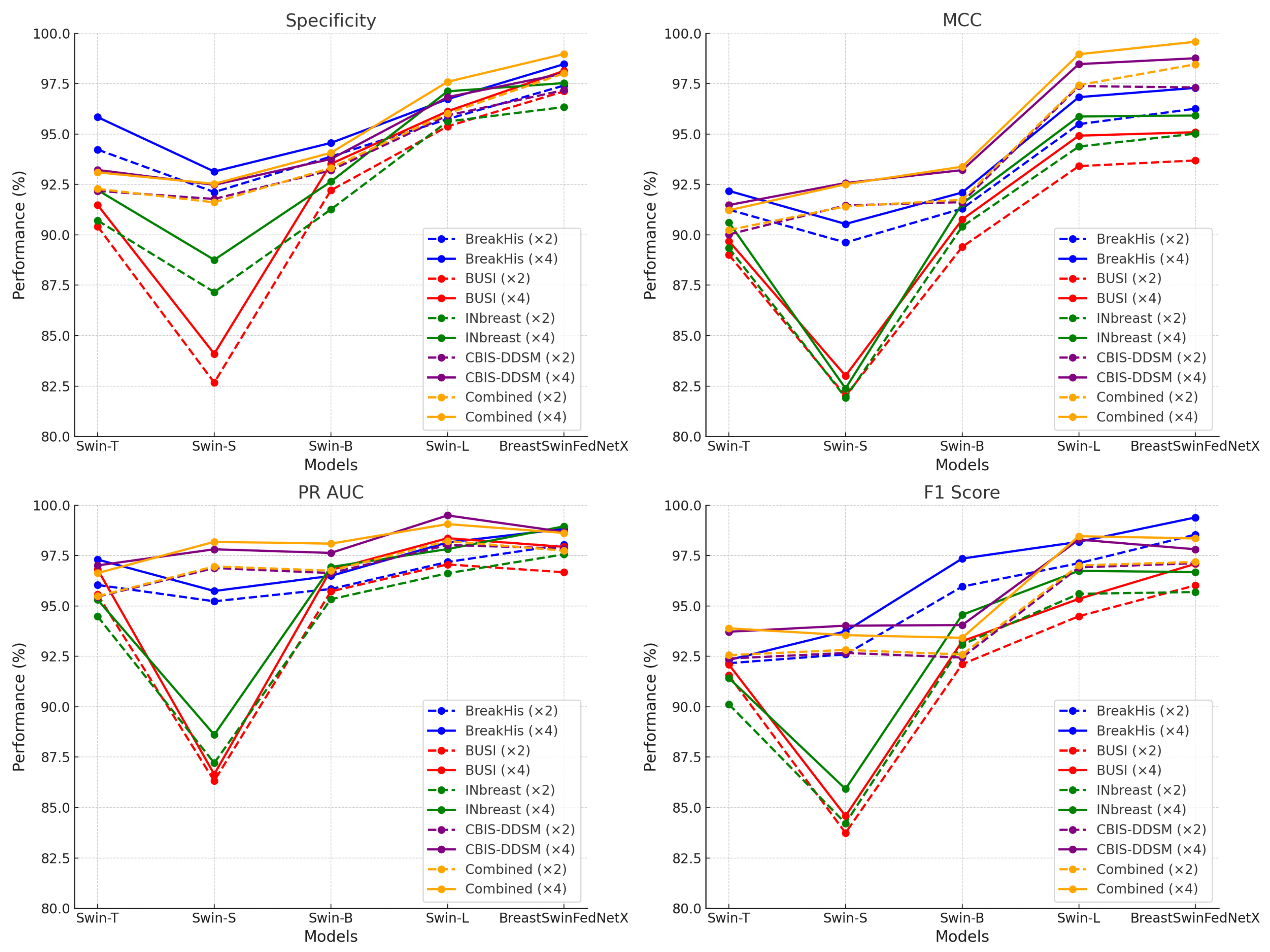
Table 8.
Performance metrics comparison across different models on augmentation (×4).
Table 8.
Performance metrics comparison across different models on augmentation (×4).
| Dataset | Metric | Swin-T | Swin-S | Swin-B | Swin-L | BreastSwinFedNetX |
|---|
| BreakHis | Specificity (%) | 95.84 ± 1.12 | 93.14 ± 1.35 | 94.56 ± 1.23 | 96.73 ± 0.94 | 98.47 ± 0.51 |
| MCC (%) | 92.18 ± 1.48 | 90.54 ± 1.72 | 92.10 ± 1.66 | 96.83 ± 1.15 | 97.29 ± 0.67 |
| PR AUC (%) | 97.30 ± 1.33 | 95.74 ± 1.41 | 96.49 ± 1.25 | 98.15 ± 1.08 | 98.82 ± 0.48 |
| F1 Score (%) | 92.32 ± 1.51 | 93.74 ± 1.29 | 97.35 ± 1.38 | 98.18 ± 1.17 | 99.39 ± 0.45 |
| BUSI | Specificity (%) | 91.48 ± 1.63 | 84.10 ± 1.74 | 93.52 ± 1.49 | 96.13 ± 1.36 | 98.14 ± 0.61 |
| MCC (%) | 89.69 ± 1.54 | 83.01 ± 1.95 | 90.76 ± 1.84 | 94.92 ± 1.23 | 95.09 ± 0.76 |
| PR AUC (%) | 96.81 ± 1.47 | 86.65 ± 1.59 | 96.79 ± 1.31 | 98.36 ± 1.12 | 97.93 ± 0.53 |
| F1 Score (%) | 92.09 ± 1.35 | 84.58 ± 1.51 | 93.25 ± 1.44 | 95.35 ± 1.32 | 97.09 ± 0.47 |
| INbreast | Specificity (%) | 92.22 ± 1.89 | 88.76 ± 1.88 | 92.64 ± 1.92 | 97.12 ± 1.07 | 97.53 ± 0.89 |
| MCC (%) | 90.62 ± 1.72 | 82.38 ± 1.91 | 91.55 ± 1.79 | 95.87 ± 1.06 | 95.92 ± 0.72 |
| PR AUC (%) | 95.31 ± 1.53 | 88.61 ± 1.44 | 96.93 ± 1.60 | 97.82 ± 1.14 | 98.95 ± 0.59 |
| F1 Score (%) | 91.42 ± 1.61 | 85.92 ± 1.68 | 94.56 ± 1.49 | 96.74 ± 1.34 | 96.68 ± 0.62 |
| CBIS-DDSM | Specificity (%) | 93.22 ± 1.27 | 92.48 ± 1.45 | 93.76 ± 1.38 | 96.83 ± 1.23 | 98.01 ± 0.41 |
| MCC (%) | 91.48 ± 1.51 | 92.57 ± 1.43 | 93.21 ± 1.55 | 98.47 ± 1.01 | 98.76 ± 0.11 |
| PR AUC (%) | 97.01 ± 1.12 | 97.81 ± 1.08 | 97.63 ± 1.19 | 99.49 ± 0.97 | 98.67 ± 0.14 |
| F1 Score (%) | 93.72 ± 1.43 | 94.02 ± 1.36 | 94.05 ± 1.48 | 98.29 ± 1.06 | 97.81 ± 0.39 |
| Combined | Specificity (%) | 93.10 ± 1.41 | 92.53 ± 1.28 | 94.07 ± 1.37 | 97.59 ± 1.18 | 98.97 ± 0.36 |
| MCC (%) | 91.22 ± 1.60 | 92.51 ± 1.49 | 93.38 ± 1.41 | 98.96 ± 1.08 | 99.58 ± 0.31 |
| PR AUC (%) | 96.63 ± 1.38 | 98.18 ± 1.27 | 98.09 ± 1.34 | 99.06 ± 0.93 | 98.62 ± 0.35 |
| F1 Score (%) | 93.89 ± 1.32 | 93.55 ± 1.22 | 93.42 ± 1.51 | 98.46 ± 1.13 | 98.35 ± 0.29 |
Table 9.
Classification report of BreastSwinFedNetX for all datasets on ×2 augmented training data.
Table 9.
Classification report of BreastSwinFedNetX for all datasets on ×2 augmented training data.
| Dataset | Class | Specificity (%) | MCC (%) | PR AUC (%) | F1 Score (%) |
|---|
| BreakHis | Adenosis | 96.91 | 97.03 | 96.56 | 96.96 |
| Fibroadenoma | 95.68 | 96.51 | 96.72 | 95.10 |
| Phyllodes Tumor | 96.60 | 95.02 | 95.85 | 95.86 |
| Tubular Adenoma | 95.58 | 95.00 | 96.32 | 95.28 |
| Ductal Carcinoma | 95.65 | 97.58 | 96.55 | 96.34 |
| Lobular Carcinoma | 96.11 | 94.92 | 95.30 | 94.88 |
| Mucinous Carcinoma | 95.96 | 96.61 | 96.50 | 96.89 |
| Papillary Carcinoma | 96.23 | 96.93 | 95.52 | 97.30 |
| BUSI | Normal | 95.84 | 95.26 | 95.31 | 96.58 |
| Benign | 96.57 | 96.38 | 95.48 | 95.44 |
| Malignant | 94.91 | 96.34 | 97.75 | 97.55 |
| INbreast | Benign | 97.49 | 94.87 | 98.40 | 95.94 |
| Malignant | 96.81 | 95.73 | 97.08 | 94.23 |
| CBIS-DDSM | Benign | 96.91 | 95.15 | 94.67 | 96.18 |
| Malignant | 95.21 | 97.40 | 95.97 | 96.38 |
| Combined | Benign | 95.71 | 96.53 | 97.34 | 97.03 |
| Malignant | 96.19 | 97.18 | 97.36 | 96.82 |
Table 10.
Classification report of BreastSwinFedNetX for all datasets on ×4 augmented training data.
Table 10.
Classification report of BreastSwinFedNetX for all datasets on ×4 augmented training data.
| Dataset | Class | Specificity (%) | MCC (%) | PR AUC (%) | F1 Score (%) |
|---|
| BreakHis | Adenosis | 99.50 | 99.19 | 98.44 | 99.42 |
| Fibroadenoma | 98.34 | 99.16 | 99.48 | 98.22 |
| Phyllodes Tumor | 99.52 | 98.29 | 99.50 | 98.66 |
| Tubular Adenoma | 98.51 | 98.78 | 99.50 | 98.15 |
| Ductal Carcinoma | 98.44 | 99.20 | 99.38 | 99.50 |
| Lobular Carcinoma | 98.71 | 98.38 | 98.01 | 98.69 |
| Mucinous Carcinoma | 99.35 | 98.23 | 99.49 | 99.06 |
| Papillary Carcinoma | 99.50 | 98.95 | 98.47 | 99.37 |
| BUSI | Normal | 98.22 | 98.70 | 98.34 | 98.63 |
| Benign | 99.24 | 98.82 | 98.76 | 98.36 |
| Malignant | 98.52 | 99.50 | 99.37 | 99.22 |
| INbreast | Benign | 98.11 | 96.50 | 99.12 | 95.51 |
| Malignant | 96.79 | 94.08 | 98.34 | 97.98 |
| CBIS-DDSM | Benign | 99.59 | 98.51 | 98.28 | 98.99 |
| Malignant | 98.31 | 99.46 | 99.25 | 99.39 |
| Combined | Benign | 98.95 | 98.46 | 99.50 | 99.38 |
| Malignant | 99.47 | 99.61 | 99.49 | 98.61 |
Table 11.
Performance comparison of individual Swin variants versus BreastSwinFedNetX.
Table 11.
Performance comparison of individual Swin variants versus BreastSwinFedNetX.
| Model Variant | Specificity (%) | F1 Score (%) | PR AUC (%) | MCC (%) |
|---|
| Swin-Base | 95.48 | 95.61 | 95.79 | 94.22 |
| Swin-Small | 96.73 | 96.85 | 96.91 | 95.78 |
| Swin-Tiny | 97.28 | 97.35 | 97.49 | 96.52 |
| Swin-Large | 97.93 | 97.88 | 98.01 | 97.17 |
| BreastSwinFedNetX | 98.97 | 98.35 | 98.62 | 98.35 |
Table 12.
Impact of meta-learner choice on final performance.
Table 12.
Impact of meta-learner choice on final performance.
| Meta-Learner | Specificity (%) | F1 Score (%) | PR AUC (%) | MCC (%) |
|---|
| Logistic Regression | 97.12 | 97.20 | 97.38 | 96.42 |
| Decision Tree | 97.67 | 97.74 | 97.81 | 96.96 |
| K-Nearest Neighbors | 96.84 | 96.91 | 97.05 | 95.70 |
| Naive Bayes | 95.52 | 95.68 | 95.81 | 94.12 |
| Support Vector Machine | 97.23 | 97.31 | 97.44 | 96.38 |
| RF | 98.97 | 98.35 | 98.62 | 98.35 |
Table 13.
Effect of preprocessing techniques on BreastSwinFedNetX performance.
Table 13.
Effect of preprocessing techniques on BreastSwinFedNetX performance.
| Preprocessing Configuration | Specificity (%) | F1 Score (%) | PR AUC (%) | MCC (%) |
|---|
| Resizing Only | 93.24 | 95.16 | 94.02 | 90.87 |
| + Normalization | 94.01 | 96.03 | 95.26 | 91.79 |
| + Noise Injection (Gaussian, = 0.01) | 94.67 | 96.71 | 96.13 | 93.14 |
| + Contrast Stretching | 95.28 | 97.22 | 97.03 | 94.05 |
| All Combined | 98.97 | 98.35 | 98.62 | 98.35 |
Table 14.
Quantitative evaluation of Grad-CAM outputs based on heatmap compactness and noise metrics on the combined dataset.
Table 14.
Quantitative evaluation of Grad-CAM outputs based on heatmap compactness and noise metrics on the combined dataset.
| Model | Activation Area (%) | Edge Density (%) | CAM Noise Ratio |
|---|
| BreastSwinFedNetX | 11.6 | 19.8 | 0.085 |
| Swin-Large | 19.2 | 27.1 | 0.158 |
| Swin-Small | 22.0 | 27.6 | 0.181 |
| Swin-Base | 24.1 | 29.3 | 0.217 |
| Swin-Tiny | 25.4 | 31.0 | 0.211 |
Table 15.
F1 Score comparison between FL-based and centralized models.
Table 15.
F1 Score comparison between FL-based and centralized models.
| Dataset | FL-Based (%) | Centralized (%) | Difference (%) |
|---|
| BreakHis | 99.39 | 99.19 | +0.20 |
| BUSI | 97.09 | 96.86 | +1.09 |
| INbreast | 96.68 | 95.56 | +1.12 |
| CBIS-DDSM | 97.81 | 97.16 | +0.65 |
| Combined Dataset | 99.02 | 98.08 | +0.94 |
Table 16.
Training time and communication overhead comparison.
Table 16.
Training time and communication overhead comparison.
| Dataset | Training Time (FL) | Training Time (Centralized) | Communication Overhead |
|---|
| BreakHis | 5.2 h | 4.8 h | Low |
| BUSI | 6.1 h | 5.2 h | Moderate |
| INbreast | 5.8 h | 5.0 h | Moderate |
| CBIS-DDSM | 5.0 h | 4.6 h | Low |
| Combined Dataset | 7.3 h | 6.4 h | High |
Table 17.
Existing work and proposed method result comparison for breast cancer classification.
Table 17.
Existing work and proposed method result comparison for breast cancer classification.
| Ref. | Method | Dataset | Result (%) | Limitations |
|---|
| [29] | CNN | INbreast | 96.50 | Overfitting, dataset limitations |
| [37] | ViT | INbreast | 98.52 | External classifier limits deployment |
| [41] | FL-L2CNN-BCDet | INbreast | 98.33 | No deployment or compliance strategy |
| [29] | ResCNN | INbreast | 96.50 | High computational cost; complex tuning |
| [24] | Inception-V3 | BreakHis | 92.00 | Class imbalance, lacks explainability |
| [39] | EAT | BreakHis | 99.00 | High complexity, data dependency |
| [34] | EfficientNetV2 + ViT | BreakHis | 98.10 | Overfitting risk |
| [32] | MaxViT | BreakHis | 92.12 | Dataset diversity, scalability |
| [42] | FL + InceptionV3 | BreakHis | 99.38 | Single dataset; poor generalization |
| [28] | GAN + CNN | BUSI | 86.00 | Dataset dependence; lacks robustness |
| [33] | CNN + ViT | BUSI | 89.43 | Weak subclass performance |
| [35] | SupCon-ViT | BUSI | 88.61 | No diverse dataset validation |
| [44] | FL + DCNN | BUSI | 98.09 | No XAI; lacks cross-dataset validation |
| [45] | CNN-based FL | BUSI | 95.50 | No interpretability; high resource needs |
| [30] | LFR-COA-DenseNet121-BC | CBIS-DDSM | 98.97 | Optimization sensitivity, dataset limitations |
| [22] | FHDF | CBIS-DDSM | 98.83 | Dataset diversity and interpretability |
| [47] | FL + DenseNet | CBIS-DDSM | 95.73 | No unified XAI; communication cost |
| Proposed—BreastSwinFedNetX |
| | | BreakHis | 99.34 ± 0.42 | |
| | | BUSI | 98.03 ± 0.55 | |
| Ours | BreastSwinFedNetX | INbreast | 98.89 ± 0.65 | Computational complexity |
| | | CBIS-DDSM | 98.58 ± 0.06 | |
Table 18.
Statistical significance comparison of BreastSwinFedNetX model on BreakHis and BUSI using paired t-test ().
Table 18.
Statistical significance comparison of BreastSwinFedNetX model on BreakHis and BUSI using paired t-test ().
| Comparison | BreakHis (p-Values) | BUSI (p-Values) |
|---|
| Specificity | F1 Score | PR AUC | MCC | Specificity | F1 Score | PR AUC | MCC |
|---|
| vs. Swin-L | 0.002 | 0.008 | 0.007 | 0.041 | 0.612 | 0.121 | 0.158 | 0.244 |
| vs. Swin-T | 0.001 | 0.004 | 0.053 | 0.076 | 0.003 | 0.003 | 0.005 | 0.003 |
| vs. Swin-S | 0.003 | 0.002 | 0.008 | 0.017 | 0.146 | 0.013 | 0.072 | 0.021 |
| vs. Swin-B | 0.693 | 0.185 | 0.101 | 0.602 | 0.005 | 0.009 | 0.003 | 0.072 |
Table 19.
Statistical significance comparison of BreastSwinFedNetX model on INbreast and CBIS-DDSM using paired t-test ().
Table 19.
Statistical significance comparison of BreastSwinFedNetX model on INbreast and CBIS-DDSM using paired t-test ().
| Comparison | INbreast (p-Values) | CBIS-DDSM (p-Values) |
|---|
| Specificity | F1 Score | PR AUC | MCC | Specificity | F1 Score | PR AUC | MCC |
|---|
| vs. Swin-L | 0.005 | 0.012 | 0.019 | 0.063 | 0.592 | 0.087 | 0.142 | 0.203 |
| vs. Swin-T | 0.002 | 0.004 | 0.048 | 0.007 | 0.008 | 0.006 | 0.005 | 0.004 |
| vs. Swin-S | 0.003 | 0.007 | 0.009 | 0.025 | 0.014 | 0.010 | 0.019 | 0.033 |
| vs. Swin-B | 0.612 | 0.198 | 0.102 | 0.479 | 0.017 | 0.013 | 0.012 | 0.006 |


 ,
, 


