
Lifecycle DoE—The Companion for a Holistic Development Process

 , ,
, ,
Abstract
:
1. Introduction
2. Materials and Methods
2.1. Optimal Designs
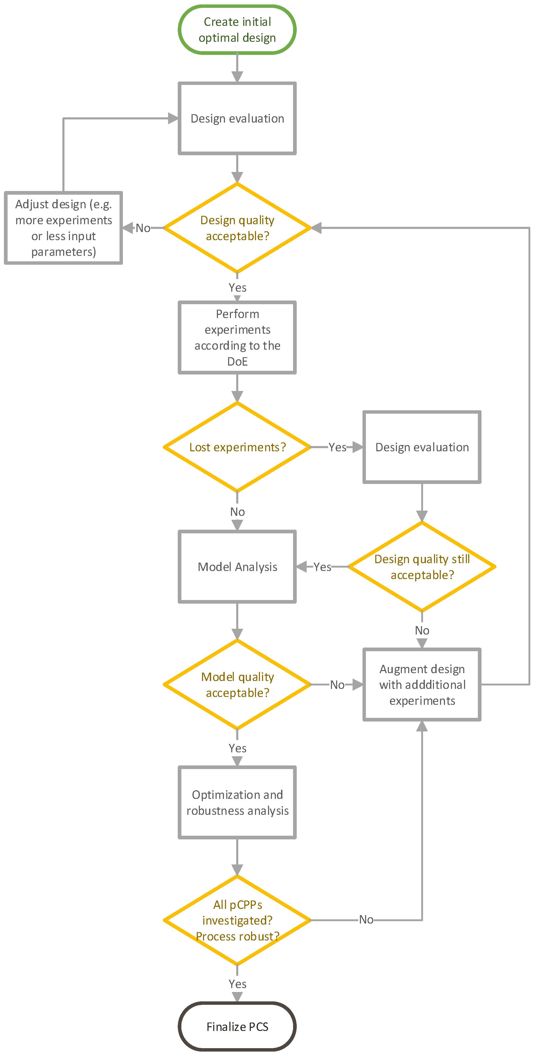
2.2. Lifecycle DoE
2.3. Design Analysis
Power Analysis
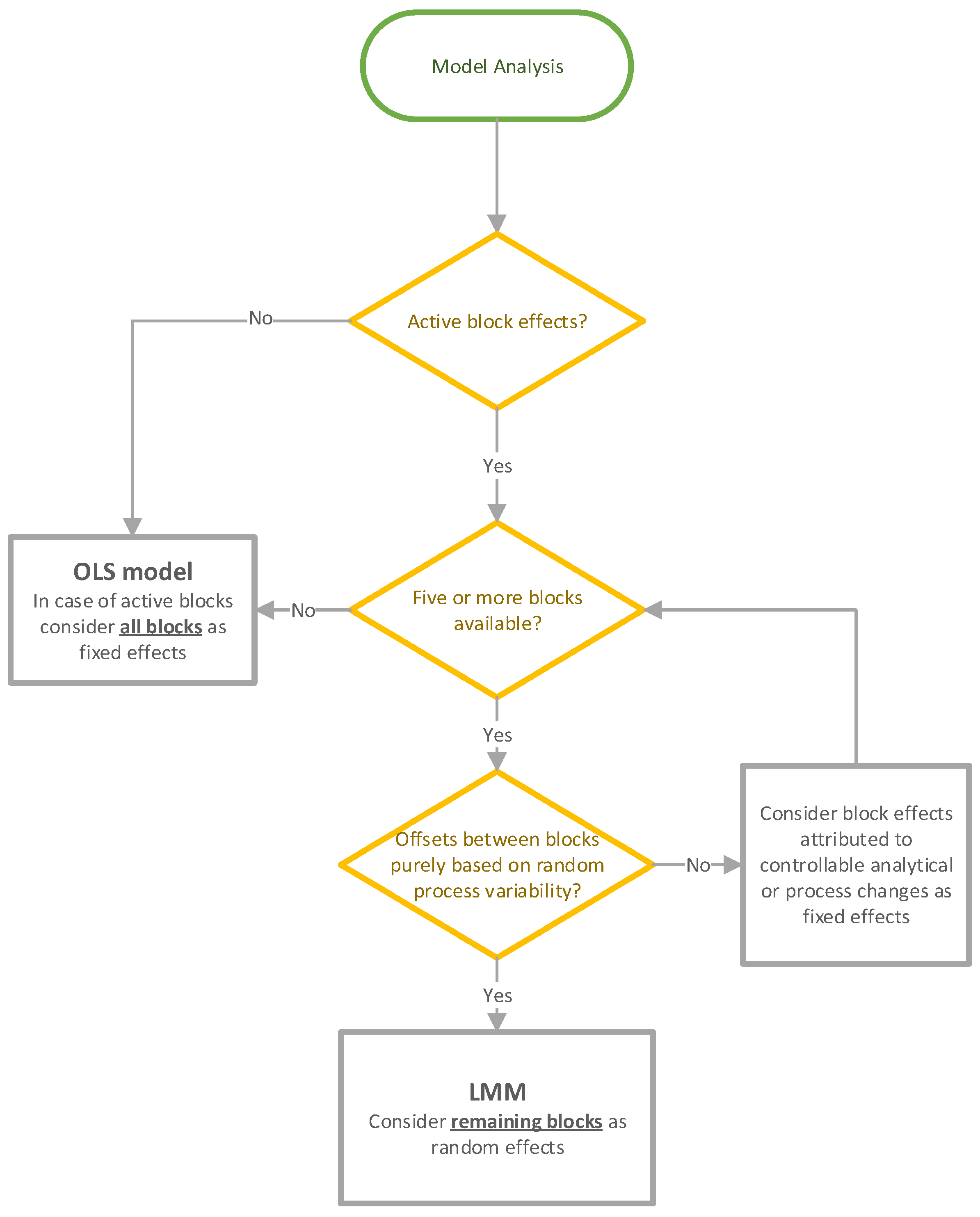
2.4. Model Analysis
2.4.1. Ordinary Least Square Models
- Y is the observed output parameter (e.g., critical quality attribute)
- is the model intercept
- is the ith main effect
- is the ijth two factor interaction effect
- is the iith quadratic effect
- is the iiith cubic effect
- is the ith fixed block effect
- x is the input parameter setting of the ith, jth or kth parameter
- is the ith block setting
- p is the number of investigated input parameters
- b is the number of fixed block effects
- is the residual error term, assuming
2.4.2. Linear Mixed Models
- was the random block term, assuming .
2.4.3. Software
2.5. Process Optimization Analysis
2.6. Process Characterization Study
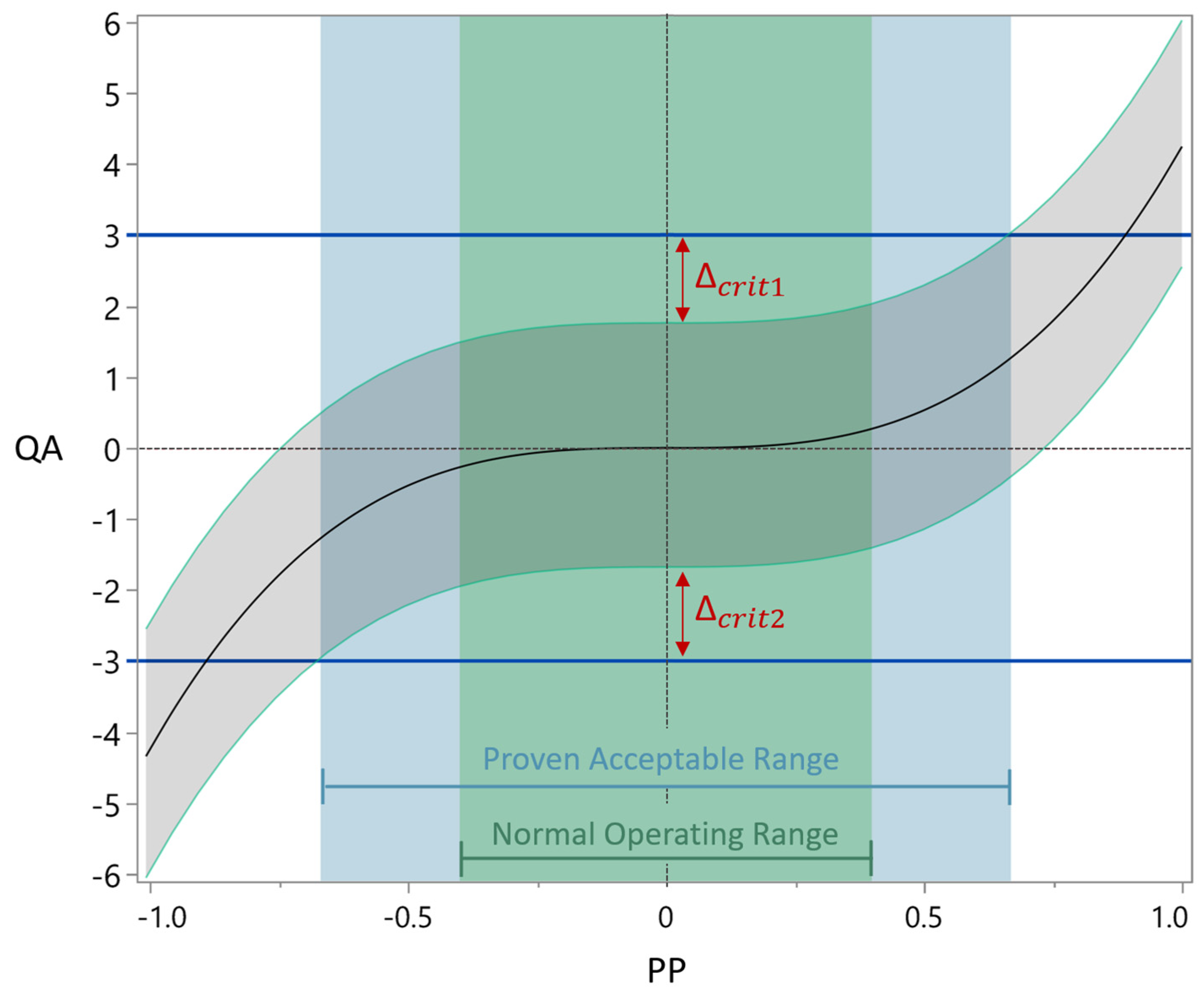
2.6.1. Acceptance Limits
2.6.2. Definition Normal Operation Ranges
2.6.3. Definition Proven Acceptable Ranges
2.6.4. Process Parameter Criticality Assessment
2.6.5. Multivariate Acceptable Ranges
2.6.6. Retrospective Power Analysis
2.7. Data
3. Results
3.1. Work Package 1
3.1.1. Design Analysis
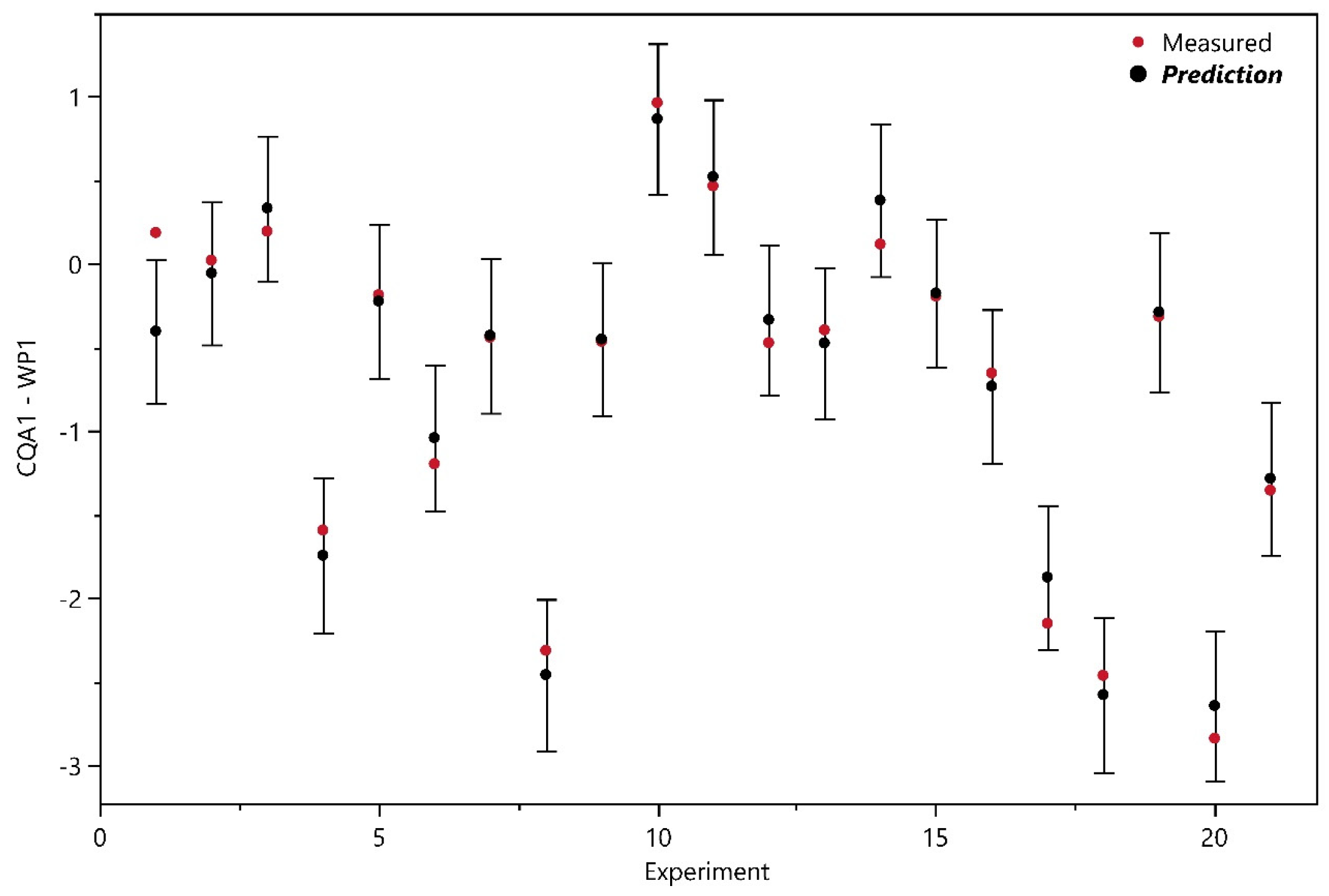
3.1.2. Model Analysis
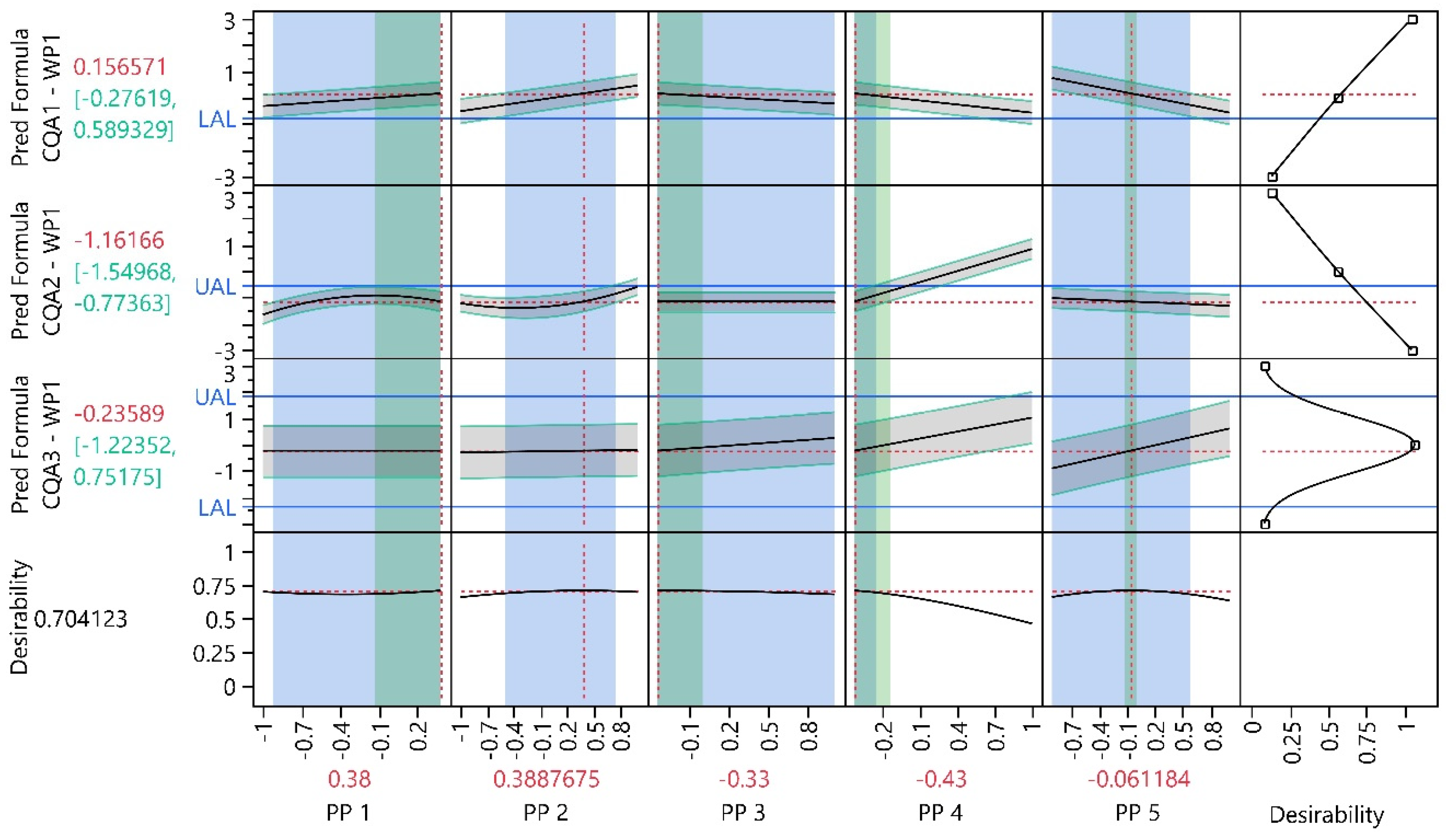
3.1.3. Process Optimization Analysis
3.1.4. Process Parameter Criticality Assessment
3.2. Work Package 1–3
3.2.1. Design Analysis
3.2.2. Model Analysis
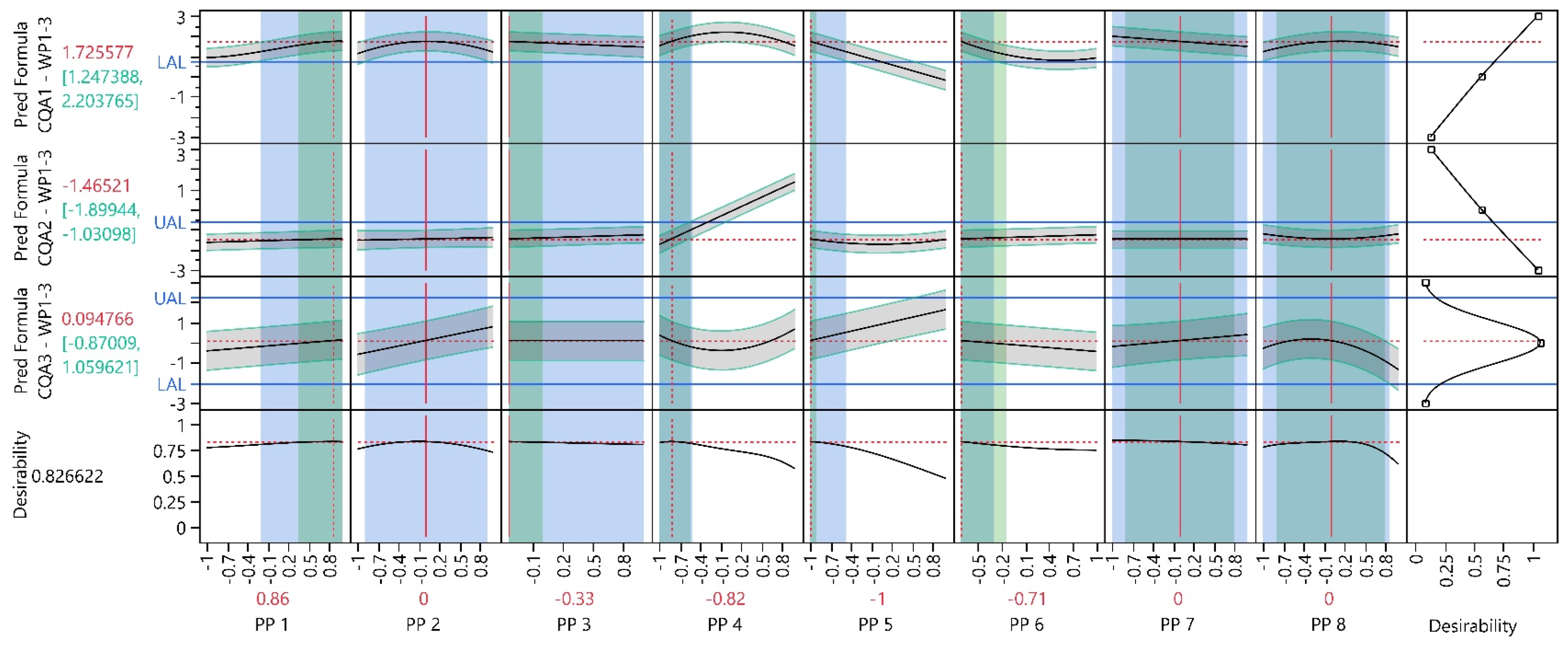
3.2.3. Process Optimization Analysis
3.2.4. Process Parameter Criticality Assessment
3.3. Work Package 1–4
3.3.1. Design Analysis
3.3.2. Model Analysis
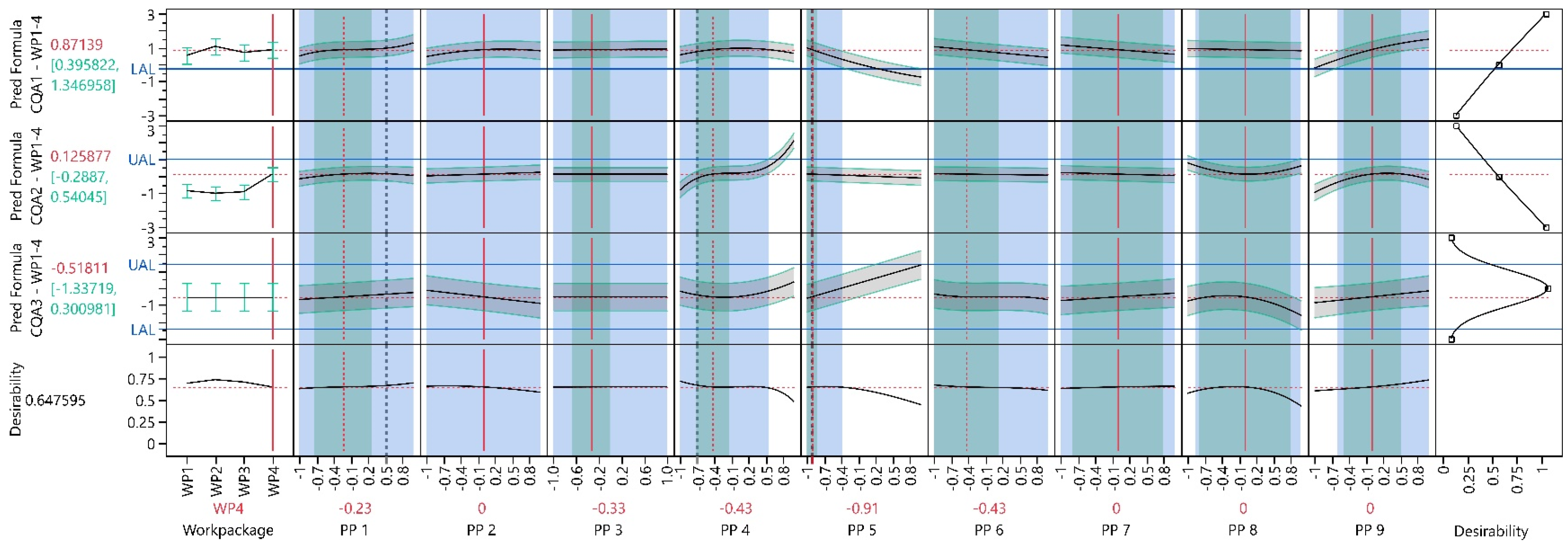
3.3.3. Process Optimization Analysis
3.3.4. Process Parameter Criticality Assessment
3.4. Work Package 1–7
3.4.1. Model Analysis
3.4.2. Retrospective Power Analysis
3.4.3. Process Characterization Study
3.4.4. Multivariate Acceptable Ranges
4. Discussion
- It is recommended to compile a list of all PPs to be optimized within development and investigated in the PCS. It is more efficient to consider all PPs in the initial phase of the LDoE rather than adding them sequentially over the WPs. This was evident in the design analysis of WP1–4, where the power of the newly added PP9 and all combinations with this parameter were below 80%. In our case, a definitive screening design [47,48] would have been appropriate to investigate the impact of all nine PPs, including three center point experiments with only 21 experiments. From there, additional design augmentation can be performed to extend the design space.
- The LDoE approach results in broader PP ranges compared to standard DoEs, increasing the risk of an edge-of-failure. An edge of failure is a PP setting combination that reproducible leads to a loss of the experiment. It is recommended to carefully inspect combinations, especially when multiple PPs are at their highest or lowest setting. Alternatively, performing test experiments upfront with the most suspicious settings is recommended.
- It is also recommended to compile a list considering all CQAs. It is crucial that data from all relevant analytical output parameters are available across the complete LDoE.
- Plan for enough retains from the experiments. In cases where analytical experiments need to be repeated or a new CQA appears within development, experiments from previous WPs would otherwise need to be repeated, dramatically increasing the resources.
- Advising against keeping PP settings fixed within one WP to save experiments. The design analysis in WP1–4 shows that many terms, including PP2 or PP3, which were kept constant in WP3, do not meet the design quality criteria regarding statistical power in the following WPs.
- It is recommended to initiate the LDoE at a stage of process development where no fundamental parameters will be changed. This is typically not the case in the very early phase of process development. Fundamental parameters are, for instance, cell lines or the medium. These parameters lead to many possible interaction effects with other PPs. While these higher-order interaction effects can theoretically be considered in the LDoE, they lead to a dramatic increase in required experiments.
- It is not recommended to include OFAT experiments into the LDoE with only one replicate. While OFAT experiments can theoretically be modeled in the form of linear or quadratic effects, without any replicate, they have a very high leverage. This leads to worse model diagnostics, for instance, the one-point cross-validation (predicted R2) loses its informative value and potential underestimation of the variance can appear.
5. Conclusions
Supplementary Materials
Author Contributions
Funding
Institutional Review Board Statement
Informed Consent Statement
Data Availability Statement
Conflicts of Interest
List of Abbreviations
| Abbrevation | Full Word |
| AICc | Akaike information criterion corrected |
| AL | acceptance limits |
| CCD | central composite design |
| CMC | chemical manufacturing and control |
| CPP | critical process parameter |
| CQA | critical quality attribute |
| DoE | Design of Experiment |
| EMA | European Medicine Agency |
| FDA | Food and Drug Administration |
| FMEA | failure mode and effects analysis |
| hpCPP | highly potentially critical process parameter |
| IPM | integrated process model |
| LDoE | Life-Cycle-DoE |
| LMM | linear mixed effect model |
| MAR | multivariate acceptable ranges |
| NOR | normal operating range |
| OFAT | one factor at a time |
| OLS | ordinary least squares |
| PAR | proven acceptable range |
| PAT | process analytical technology |
| pCPP | potential critical process parameter |
| pCQA | potential critical quality attribute |
| PCS | process characterization study |
| PI | prediction interval |
| PP | process parameter |
| pPAR | preliminary proven acceptable range |
| PvM | prediction-versus-measured |
| QbD | Quality by Design |
| REML | restricted maximum likelihood |
| RMSE | root mean square error |
| SD | standard deviation |
| SME | subject matter expert |
| WP | work package |
References
- Kontoravdi, C.; Samsatli, N.J.; Shah, N. Development and Design of Bio-Pharmaceutical Processes. Curr. Opin. Chem. Eng. 2013, 2, 435–441. [Google Scholar] [CrossRef]
- Mandenius, C.-F.; Brundin, A. Review: Biocatalysts and Bioreactor Design, Bioprocess Optimization, Using Design-of-Experiments Methodology. Biotechnol. Progr. 2008, 24, 1191–1203. [Google Scholar] [CrossRef] [PubMed]
- Politis, S.N.; Colombo, P.; Colombo, G.; Rekkas, D.M. Design of Experiments (DoE) in Pharmaceutical Development. Drug Dev. Ind. Pharm. 2017, 43, 889–901. [Google Scholar] [CrossRef] [PubMed]
- Gullberg, J.; Jonsson, P.; Nordström, A.; Sjöström, M.; Moritz, T. Design of Experiments: An Effcient Strategy to Identify Factors Infuencing Extraction and Derivatization of Arabidopsis Thaliana Samples in Metabolomic Studies with Gas Chromatography/Mass Spectrometry. Anal. Biochem. 2004, 331, 283–295. [Google Scholar] [CrossRef]
- Kroll, P.; Hofer, A.; Ulonska, S.; Kager, J.; Herwig, C. Model-Based Methods in the Biopharmaceutical Process Lifecycle. Pharm. Res. 2017, 34, 2596–2613. [Google Scholar] [CrossRef]
- Hsueh, K.L.; Lin, T.Y.; Lee, M.T.; Hsiao, Y.Y.; Gu, Y. Design of Experiments for Modeling of Fermentation Process Characterization in Biological Drug Production. Processes 2022, 10, 237. [Google Scholar] [CrossRef]
- Kasemiire, A.; Avohou, H.T.; De Bleye, C.; Sacre, P.Y.; Dumont, E.; Hubert, P.; Ziemons, E. Design of Experiments and Design Space Approaches in the Pharmaceutical Bioprocess Optimization. Eur. J. Pharm. Biopharm. 2021, 166, 144–154. [Google Scholar] [CrossRef]
- Beg, S.; Swain, S.; Rahman, M.; Hasnain, M.S.; Imam, S.S. Application of Design of Experiments (DoE) in Pharmaceutical Product and Process Optimization. In Pharmaceutical Quality by Design; Academic Press: Cambridge, MA, USA, 2019; pp. 43–64. [Google Scholar] [CrossRef]
- FDA. Pharmaceutical CGMPs for the 21St Century; US Food & Drug Administration: Silver Spring, MD, USA, 2004; p. 32.
- International Council for Harmonisation ICH Topic Q 8 (R2) Pharmaceutical Development; EMA: London, UK, 2017.
- Rathore, A.S.; Winkle, H. Quality-by-Design Approach. Nat. Biotechnol. 2009, 27, 26–34. [Google Scholar] [CrossRef]
- Kunzelmann, M.; Thoma, J.; Laibacher, S.; Studts, J.M.; Presser, B.; Spitz, J. An In-silico Approach towards Multivariate Acceptable Ranges in Biopharmaceutical Manufacturing. AAPS Open 2024, 10, 7. [Google Scholar] [CrossRef]
- Little, T.A. Process Characterization Essentials: Process Understanding and Health Authorities Guidance; BioPharm International: East Windsor, NJ, USA, 2017; Volume 30, ISBN 8776525295. [Google Scholar]
- Fukuda, I.M.; Pinto, C.F.F.; Moreira, C.D.S.; Saviano, A.M.; Lourenço, F.R. Design of Experiments (DoE) Applied to Pharmaceutical and Analytical Quality by Design (QbD). Braz. J. Pharm. Sci. 2018, 54, 1–16. [Google Scholar] [CrossRef]
- Sommeregger, W.; Sissolak, B.; Kandra, K.; von Stosch, M.; Mayer, M.; Striedner, G. Quality by Control: Towards Model Predictive Control of Mammalian Cell Culture Bioprocesses. Biotechnol. J. 2017, 12, 1600546. [Google Scholar] [CrossRef] [PubMed]
- Shekhawat, L.K.; Godara, A.; Kumar, V.; Rathore, A.S. Design of Experiments Applications in Bioprocessing: Chromatography Process Development Using Split Design of Experiments. Biotechnol. Prog. 2019, 35, e2730. [Google Scholar] [CrossRef] [PubMed]
- Zahel, T.; Hauer, S.; Mueller, E.M.; Murphy, P.; Abad, S.; Vasilieva, E.; Maurer, D.; Brocard, C.; Reinisch, D.; Sagmeister, P.; et al. Integrated Process Modeling—A Process Validation Life Cycle Companion. Bioengineering 2017, 4, 86. [Google Scholar] [CrossRef] [PubMed]
- Oberleitner, T.; Zahel, T.; Pretzner, B.; Herwig, C. Holistic Design of Experiments Using an Integrated Process Model. Bioengineering 2022, 9, 643. [Google Scholar] [CrossRef]
- Schmieder, V.; Fieder, J.; Drerup, R.; Gutierrez, E.A.; Guelch, C.; Stolzenberger, J.; Stumbaum, M.; Mueller, V.S.; Higel, F.; Bergbauer, M.; et al. Towards Maximum Acceleration of Monoclonal Antibody Development: Leveraging Transposase-Mediated Cell Line Generation to Enable GMP Manufacturing within 3 Months Using a Stable Pool. J. Biotechnol. 2022, 349, 53–64. [Google Scholar] [CrossRef]
- Zhang, Z.; Chen, J.; Wang, J.; Gao, Q.; Ma, Z.; Xu, S.; Zhang, L.; Cai, J.; Zhou, W. Reshaping Cell Line Development and CMC Strategy for Fast Responses to Pandemic Outbreak. Biotechnol. Prog. 2021, 37, 1–10. [Google Scholar] [CrossRef]
- Kelley, B. Developing Therapeutic Monoclonal Antibodies at Pandemic Pace. Nat. Biotechnol. 2020, 38, 540–545. [Google Scholar] [CrossRef]
- Bolisetty, P.; Tremml, G.; Xu, S.; Khetan, A. Enabling Speed to Clinic for Monoclonal Antibody Programs Using a Pool of Clones for IND-Enabling Toxicity Studies. Mabs 2020, 12, 1763727. [Google Scholar] [CrossRef]
- Xu, J.; Ou, J.; McHugh, K.P.; Borys, M.C.; Khetan, A. Upstream Cell Culture Process Characterization and In-Process Control Strategy Development at Pandemic Speed. MAbs 2022, 14, 2060724. [Google Scholar] [CrossRef]
- Hakemeyer, C.; McKnight, N.; St. John, R.; Meier, S.; Trexler-Schmidt, M.; Kelley, B.; Zettl, F.; Puskeiler, R.; Kleinjans, A.; Lim, F.; et al. Process Characterization and Design Space Definition. Biologicals 2016, 44, 306–318. [Google Scholar] [CrossRef]
- Jankovic, A.; Chaudhary, G.; Goia, F. Designing the Design of Experiments (DOE)—An Investigation on the Influence of Different Factorial Designs on the Characterization of Complex Systems. Energy Build. 2021, 250, 111298. [Google Scholar] [CrossRef]
- Souza, J.P.E.; Alves, J.M.; Damiani, J.H.S.; Silva, M.B. Design of Experiments: Its Importance in the Efficient Project Management. In Proceedings of the 22nd International Conference on Production Research, Iguassu Falls, Brazil, 28 July–1 August 2013. [Google Scholar] [CrossRef]
- Atwood, C.L. Optimal and Effcient Designs of Experiments. Ann. Math. Stat. 1969, 40, 1570–1602. [Google Scholar] [CrossRef]
- Sanchez, S.M.; Wan, H. Better than Petaflop: The Power of Efficient Experimental Design. In Proceedings of the 2009 Winter Simulation Conference (WSC), Austin, TX, USA, 13–16 December 2009; pp. 60–74. [Google Scholar]
- Douglas, C. Montgomery Montgomery: Design and Analysis of Experiments, 9th ed.; John Wiley & Sons, Inc.: Hoboken, NJ, USA, 2017; ISBN 9781119113478. [Google Scholar]
- Goos, P.; Jones, B. Optimal Design of Experiments: A Case Study Approach; John Wiley and Sons: Chichester, UK, 2011; ISBN 9780470744611. [Google Scholar]
- Johnson, R.T.; Montgomery, D.C.; Jones, B.A. An Expository Paper on Optimal Design. Qual. Eng. 2011, 23, 287–301. [Google Scholar] [CrossRef]
- de Aguiar, P.F.; Bourguignon, B.; Khots, M.S.; Massart, D.L.; Phan-Than-Luu, R. D-Optimal Designs. Chemom. Intell. Lab. Syst. 1995, 30, 199–210. [Google Scholar] [CrossRef]
- Jones, B.; Allen-Moyer, K.; Goos, P. A-Optimal versus D-Optimal Design of Screening Experiments. J. Qual. Technol. 2021, 53, 369–382. [Google Scholar] [CrossRef]
- Goos, P.; Jones, B.; Syafitri, U. I-Optimal Design of Mixture Experiments. J. Am. Stat. Assoc. 2016, 111, 899–911. [Google Scholar] [CrossRef]
- Ledolter, J.; Kardon, R.H. Focus on Data: Statistical Design of Experiments and Sample Size Selection Using Power Analysis. Investig. Ophthalmol. Vis. Sci. 2020, 61. [Google Scholar] [CrossRef]
- Perugini, M.; Gallucci, M.; Costantini, G. A Practical Primer to Power Analysis for Simple Experimental Designs. Int. Rev. Soc. Psychol. 2018, 31, 1–23. [Google Scholar] [CrossRef]
- JMP Statistical Discovery LLC 2024. JMP® 18 Design of Experiments Guide; JMP: Cary, NC, USA, 2024. [Google Scholar]
- Oberleitner, T.; Zahel, T.; Kunzelmann, M.; Thoma, J.; Herwig, C. Incorporating Random Effects in Biopharmaceutical Control Strategies. AAPS Open 2023, 9, 4. [Google Scholar] [CrossRef]
- EMA. Preliminary QIG Considerations Regarding Pharmaceutical Process Models; EMA: London, UK, 2024; Vol. 31. [Google Scholar]
- JMP Statistical Discovery LLC 2024. JMP® 18 Fitting Linear Models; JMP: Cary, NC, USA, 2024. [Google Scholar]
- Geary, R.C. The Distribution of “Student’s” Ratio for Non-Normal Samples. Suppl. J. R. Stat. Soc. 1936, 3, 178. [Google Scholar] [CrossRef]
- Piepho, H.P.; Büchse, A.; Emrich, K. A Hitchhiker’s Guide to Mixed Models for Randomized Experiments. J. Agron. Crop Sci. 2003, 189, 310–322. [Google Scholar] [CrossRef]
- JMP Statistical Discovery LLC 2024. JMP® 18 Profilers; JMP: Cary, NC, USA, 2024. [Google Scholar]
- EMA Questions and Answers: Improving the Understanding of NORs, PARs, DSp and Normal Variability of Process Parameters; EMA: London, UK, 2017.
- Oberleitner, T.; Zahel, T.; Herwig, C. A Method for Finding a Design Space as Linear Combinations of Parameter Ranges for Biopharmaceutical Development. Comput. Aided Chem. Eng. 2023, 52, 909–914. [Google Scholar] [CrossRef]
- Zhang, Y.; Hedo, R.; Rivera, A.; Rull, R.; Richardson, S.; Tu, X.M. Post Hoc Power Analysis: Is It an Informative and Meaningful Analysis? Gen. Psychiatry 2019, 32, 3–6. [Google Scholar] [CrossRef] [PubMed]
- Jones, B.; Nachtsheim, C.J. A Class of Three-Level Designs for Definitive Screening in the Presence of Second-Order Effects. J. Qual. Technol. 2011, 43, 1–15. [Google Scholar] [CrossRef]
- Hocharoen, L.; Noppiboon, S.; Kitsubun, P. Process Characterization by Definitive Screening Design Approach on DNA Vaccine Production. Front. Bioeng. Biotechnol. 2020, 8, 574809. [Google Scholar] [CrossRef]

| Process Parameter | WP1 21 Experiments | WP1-3 59 Experiments | WP1-5 91 Experiments | WP1-7 97 Experiments |
|---|---|---|---|---|
| PP1 | [−1.00, +0.38] | [1.00, +1.00] | [1.00, +1.00] | [1.00, +1.00] |
| PP2 | [−1.00, +1.00] | [−1.00, +1.00] | [1.00, +1.00] | [1.00, +1.00] |
| PP3 | [−0.33, +1.00] | [−0.33, +1.00] | [1.00, +1.00] | [1.00, +1.00] |
| PP4 | [−0.43, +1.00] | [−1.00, +1.00] | [1.00, +1.00] | [1.00, +1.00] |
| PP5 | [−0.91, +1.00] | [−1.00, +1.00] | [1.00, +1.00] | [1.00, +1.00] |
| PP6 | +0.14 | [−0.71, +1.00] | [1.00, +1.00] | [1.00, +1.00] |
| PP7 | 0 | [−1.00, +1.00] | [1.00, +1.00] | [1.00, +1.00] |
| PP8 | 0 | [−1.00, +1.00] | [1.00, +1.00] | [1.00, +1.00] |
| PP9 | 0 | 0 | [1.00, +1.00] | [1.00, +1.00] |
| Process Parameter | Lower Limit | Upper Limit | Number of Levels |
|---|---|---|---|
| PP1 | −1.00 | +0.38 | 4 |
| PP2 | −1.00 | +1.00 | 3 |
| PP3 | −0.33 | +1.00 | 2 |
| PP4 | −0.43 | +1.00 | 2 |
| PP5 | −0.91 | +1.00 | 2 |
| Model—WP | Model Type | n | RMSE | R2 | R2 Adjusted | R2 Predicted | Heterosk. | Normally Distributed Residuals | Number of Experiments outside the 90% PI |
|---|---|---|---|---|---|---|---|---|---|
| CQA1—WP1 | OLS | 21 | 0.222 | 0.968 | 0.955 | 0.941 | no | yes | 1 |
| CQA2—WP1 | OLS | 21 | 0.161 | 0.985 | 0.977 | 0.959 | no | yes | 0 |
| CQA3—WP1 | OLS | 21 | 0.525 | 0.820 | 0.760 | 0.622 | no | yes | 0 |
| CQA1—WP1–3 | OLS | 59 | 0.245 | 0.954 | 0.936 | 0.913 | no | yes | 2 |
| CQA2—WP1–3 | OLS | 59 | 0.225 | 0.972 | 0.964 | 0.954 | no | yes | 1 |
| CQA3—WP1–3 | OLS | 59 | 0.539 | 0.801 | 0.731 | 0.577 | no | yes | 2 |
| CQA1—WP1–4 | OLS | 81 | 0.267 | 0.945 | 0.925 | 0.897 | no | yes | 2 |
| CQA2—WP1–4 | OLS | 81 | 0.231 | 0.967 | 0.954 | 0.918 | no | yes | 3 |
| CQA3—WP1–4 | OLS | 81 | 0.478 | 0.815 | 0.735 | 0.579 | no | yes | 2 |
| CQA1—WP1–7 | OLS | 97 | 0.262 | 0.946 | 0.931 | 0.910 | no | yes | 2 |
| CQA2—WP1–7 | OLS | 97 | 0.229 | 0.962 | 0.947 | 0.912 | no | yes | 5 |
| CQA3—WP1–7 | OLS | 97 | 0.445 | 0.866 | 0.802 | 0.662 | no | yes | 1 |
| CQA1—WP1–7 | LMM | 97 | 0.262 | 0.946 | 0.936 | NA | no | yes | 1 |
| CQA2—WP1–7 | LMM | 97 | 0.229 | 0.962 | 0.951 | NA | no | yes | 2 |
| CQA3—WP1–7 | LMM | 97 | 0.444 | 0.866 | 0.816 | NA | no | yes | 4 |
| Process Parameter | Target | NOR Lower | NOR Upper | pPAR Lower | pPAR Upper | Lower PAR–NOR Ratio | Upper PAR–NOR Ratio | CQA Limiting Lower pPAR | CQA Limiting Upper pPAR |
|---|---|---|---|---|---|---|---|---|---|
| PP1 | 0.38 | −0.12 | 0.88 | −0.92 | 0.38 | 2.60 | 0.00 | CQA1 | NA |
| PP2 | 0.39 | NA | NA | −0.5 | 0.76 | NA | NA | CQA1 | CQA2 |
| PP3 | −0.33 | −0.67 | 0.01 | −0.33 | 1 | 0.00 | 3.91 | NA | NA |
| PP4 | −0.43 | −0.72 | −0.14 | −0.43 | -0.25 | 0.00 | 0.62 | NA | CQA2 |
| PP5 | −0.06 | −0.15 | 0.03 | −0.91 | 0.58 | 9.44 | 7.11 | NA | CQA1 |
| Process Parameter | Lower Limit | Upper Limit | Number of Levels |
|---|---|---|---|
| PP1 | −1.00 | +1.00 | 5 |
| PP2 | −1.00 | +1.00 | 3 |
| PP3 | −0.33 | +1.00 | 2 |
| PP4 | −1.00 | +1.00 | 3 |
| PP5 | −1.00 | +1.00 | 3 |
| PP6 | −0.71 | +1.00 | 3 |
| PP7 | −1.00 | +1.00 | 3 |
| PP8 | −1.00 | +1.00 | 3 |
| Process Parameter | Target | NOR Lower | NOR Upper | pPAR Lower | pPAR Upper | Lower PAR–NOR Ratio | Upper PAR–NOR Ratio | CQA Limiting Lower pPAR | CQA Limiting Upper pPAR |
|---|---|---|---|---|---|---|---|---|---|
| PP1 | 0.86 | 0.36 | 1.36 | −0.21 | 1.00 | 2.14 | 0.28 | CQA1 | NA |
| PP2 | 0.00 | NA | NA | −0.82 | 0.90 | NA | NA | CQA1 | CQA1 |
| PP3 | −0.33 | −0.67 | 0.01 | −0.33 | 1.00 | 0.00 | 3.91 | NA | NA |
| PP4 | −0.82 | −1.11 | −0.53 | −1.00 | −0.52 | 0.62 | 1.03 | NA | CQA2 |
| PP5 | −1.00 | −1.09 | −0.91 | −1.00 | −0.47 | 0.00 | 5.89 | NA | CQA1 |
| PP6 | −0.71 | −1.28 | −0.14 | −0.71 | −0.30 | 0.00 | 0.72 | NA | CQA1 |
| PP7 | 0.00 | −0.80 | 0.80 | −1.00 | 1.00 | 1.25 | 1.25 | NA | NA |
| PP8 | 0.00 | −0.80 | 0.80 | −1.00 | 0.86 | 1.25 | 1.08 | CQA3 | NA |
| Process Parameter | Lower Limit | Upper Limit | Number of Levels |
|---|---|---|---|
| PP1 | −1.00 | +1.00 | 5 |
| PP2 | −1.00 | +1.00 | 3 |
| PP3 | −1.00 | +1.00 | 4 |
| PP4 | −1.00 | +1.00 | 5 |
| PP5 | −1.00 | +1.00 | 3 |
| PP6 | −1.00 | +1.00 | 4 |
| PP7 | −1.00 | +1.00 | 3 |
| PP8 | −1.00 | +1.00 | 3 |
| PP9 | −1.00 | +1.00 | 3 |
| Process Parameter | Target | NOR Lower | NOR Upper | pPAR Lower | pPAR Upper | Lower PAR–NOR Ratio | Upper PAR–NOR Ratio | CQA Limiting Lower pPAR | CQA Limiting Upper pPAR |
|---|---|---|---|---|---|---|---|---|---|
| PP1 | −0.23 | −0.73 | 0.27 | −1.00 | 1.00 | 1.54 | 2.46 | NA | NA |
| PP2 | 0.00 | NA | NA | −1.00 | 1.00 | NA | NA | NA | NA |
| PP3 | −0.33 | −0.67 | 0.01 | −1.00 | 1.00 | 1.97 | 3.91 | NA | NA |
| PP4 | −0.43 | −0.72 | −0.14 | −1.00 | 0.56 | 1.97 | 3.41 | NA | CQA2 |
| PP5 | −0.91 | −1.00 | −0.82 | −1.00 | −0.38 | 1.00 | 5.89 | NA | CQA1 |
| PP6 | −0.43 | −1.00 | 0.14 | −1.00 | 1.00 | 1.00 | 2.51 | NA | NA |
| PP7 | 0.00 | −0.80 | 0.80 | −1.00 | 1.00 | 1.25 | 1.25 | NA | NA |
| PP8 | 0.00 | −0.80 | 0.80 | −0.86 | 0.98 | 1.08 | 1.23 | CQA2 | CQA2 |
| PP9 | 0.00 | −0.50 | 0.50 | −0.59 | 1.00 | 1.18 | 2.00 | CQA1 | NA |
| CQA | Acceptance Limit | 90% PI | |||
|---|---|---|---|---|---|
| CQA1 | −0.98 | 0.02 | 1.00 | 0.48 | 2.09 |
| CQA2 | 1.72 | 0.95 | 0.77 | 0.38 | 2.03 |
| CQA3 | 1.60 | 0.33 | 1.27 | 0.57 | 2.22 |
| Process Parameter | Target | NOR Lower | NOR Upper | pPAR Lower | pPAR Upper | Lower PAR–NOR Ratio | Upper PAR–NOR Ratio | CQA Limiting Lower pPAR | CQA Limiting Upper pPAR |
|---|---|---|---|---|---|---|---|---|---|
| PP1 | −0.23 | −0.73 | 0.27 | −1.00 | 1.00 | 1.54 | 2.46 | NA | NA |
| PP2 | 0.00 | NA | NA | −1.00 | 1.00 | NA | NA | NA | NA |
| PP3 | −0.33 | −0.67 | 0.01 | −1.00 | 1.00 | 1.97 | 3.91 | NA | NA |
| PP4 | −0.43 | −0.72 | −0.14 | −1.00 | 0.68 | 1.97 | 3.83 | NA | CQA2 |
| PP5 | −0.91 | −1.00 | −0.82 | −1.00 | 0.26 | 1.00 | 13.00 | NA | CQA1 |
| PP6 | −0.43 | −1.00 | 0.14 | −1.00 | 1.00 | 1.00 | 2.51 | NA | NA |
| PP7 | 0.00 | −0.80 | 0.80 | −1.00 | 1.00 | 1.25 | 1.25 | NA | NA |
| PP8 | 0.00 | −0.80 | 0.80 | −1.00 | 1.00 | 1.25 | 1.25 | NA | NA |
| PP9 | 0.00 | −0.50 | 0.50 | −0.75 | 1.00 | 1.50 | 2.00 | CQA1 | NA |
Disclaimer/Publisher’s Note: The statements, opinions and data contained in all publications are solely those of the individual author(s) and contributor(s) and not of MDPI and/or the editor(s). MDPI and/or the editor(s) disclaim responsibility for any injury to people or property resulting from any ideas, methods, instructions or products referred to in the content. |
© 2024 by the authors. Licensee MDPI, Basel, Switzerland. This article is an open access article distributed under the terms and conditions of the Creative Commons Attribution (CC BY) license (https://creativecommons.org/licenses/by/4.0/).
Share and Cite
Kunzelmann, M.; Wittmann, A.; Presser, B.; Brosig, P.; Marhoffer, P.K.; Haider, M.A.; Martin, J.; Berger, M.; Wucherpfennig, T. Lifecycle DoE—The Companion for a Holistic Development Process. Bioengineering 2024, 11, 1089. https://doi.org/10.3390/bioengineering11111089
Kunzelmann M, Wittmann A, Presser B, Brosig P, Marhoffer PK, Haider MA, Martin J, Berger M, Wucherpfennig T. Lifecycle DoE—The Companion for a Holistic Development Process. Bioengineering. 2024; 11(11):1089. https://doi.org/10.3390/bioengineering11111089
Chicago/Turabian StyleKunzelmann, Marco, Anja Wittmann, Beate Presser, Philipp Brosig, Pia Kristin Marhoffer, Marlene Antje Haider, Julia Martin, Martina Berger, and Thomas Wucherpfennig. 2024. "Lifecycle DoE—The Companion for a Holistic Development Process" Bioengineering 11, no. 11: 1089. https://doi.org/10.3390/bioengineering11111089
APA StyleKunzelmann, M., Wittmann, A., Presser, B., Brosig, P., Marhoffer, P. K., Haider, M. A., Martin, J., Berger, M., & Wucherpfennig, T. (2024). Lifecycle DoE—The Companion for a Holistic Development Process. Bioengineering, 11(11), 1089. https://doi.org/10.3390/bioengineering11111089