
Optimizing Skin Cancer Survival Prediction with Ensemble Techniques

 , ,
, ,  ,
,
Abstract
:1. Introduction
- We evaluated various techniques for SKCM prediction considering their suitability and effectiveness in this context.
- We used RFE, FFE, and BFE features for ensemble methods.
- We analyzed the overall survival (OS) analysis and progression through the Kaplan–Meier estimator and the Cox hazard proportional regression model.
- We used eight baseline classifiers, namely, random forest (RF), decision tree (DT), gradient boosting (GB), AdaBoost, Gaussian naïve Bayes (GNB), extra tree (ET), logistic regression (LR), and light GBM in this research work.
- We applied ML algorithms for predicting the disease with various selected features.
- We trained four ensemble learning methods, including stacking, bagging, boosting, and voting, to achieve the best results.
2. Related Work
Limitations of Existing Studies
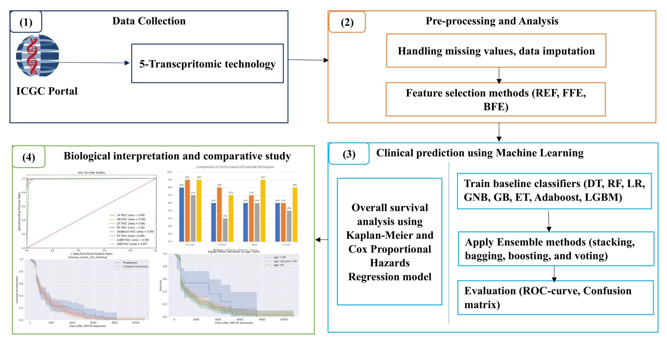
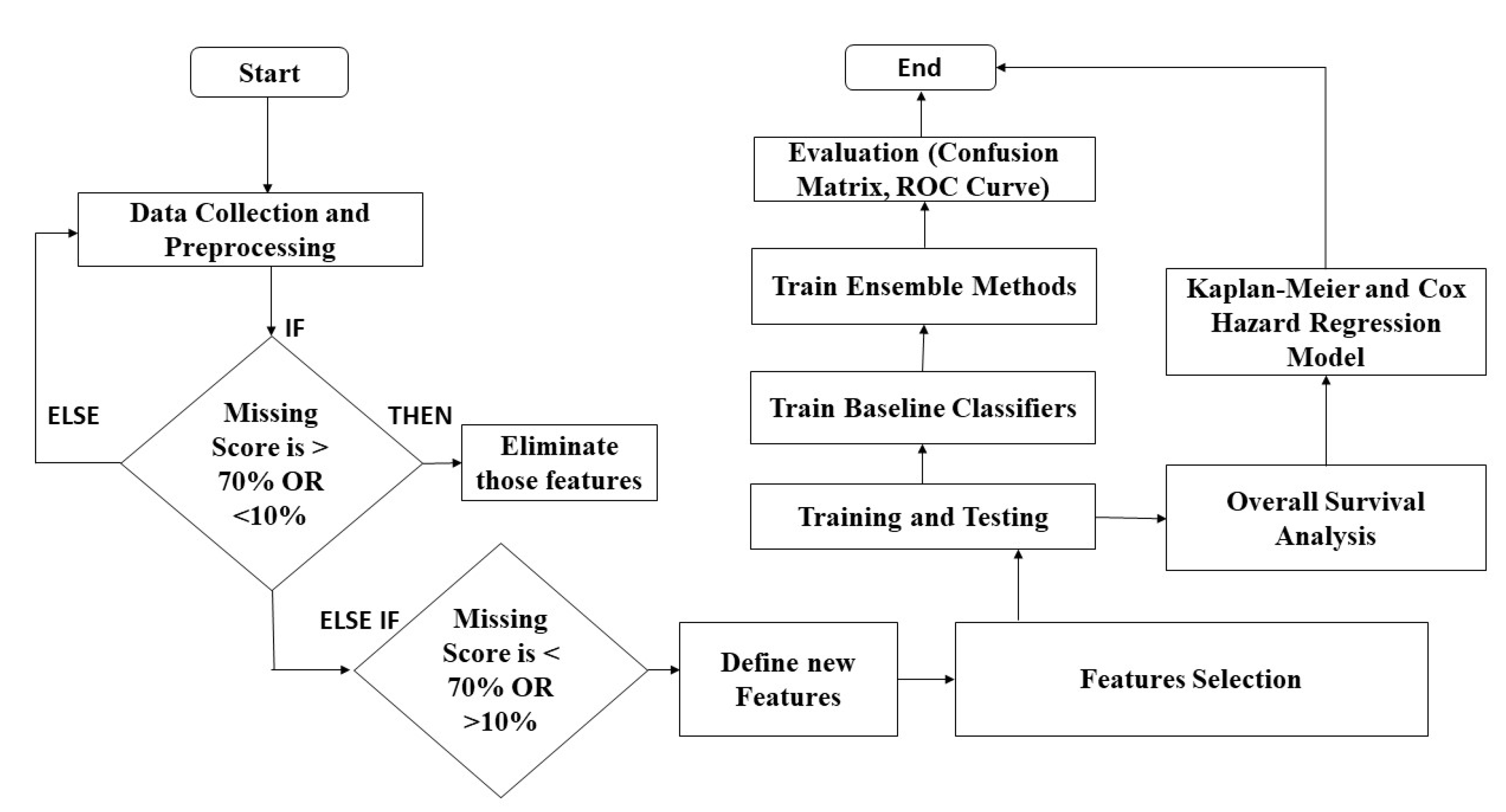
3. Materials and Methods
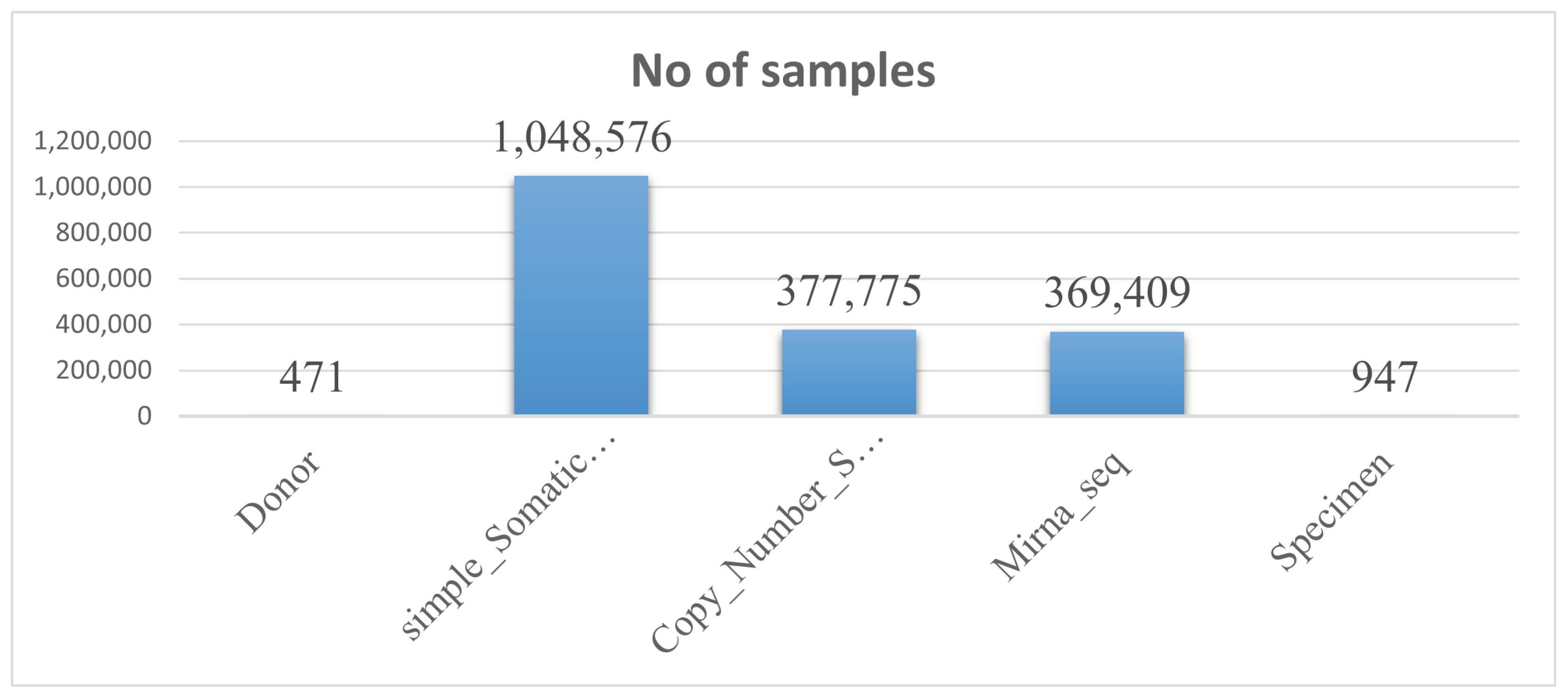
3.1. Dataset Collection
3.2. Preprocessing
Feature Selection
| Algorithm 1 Forward feature elimination. |
|
| Algorithm 2 Backward feature elimination. |
|
| Algorithm 3 Recursive feature elimination. |
|
3.3. Proposed Methodology
| Algorithm 4 ML-based ensemble methods. |
|
4. Experimental Results
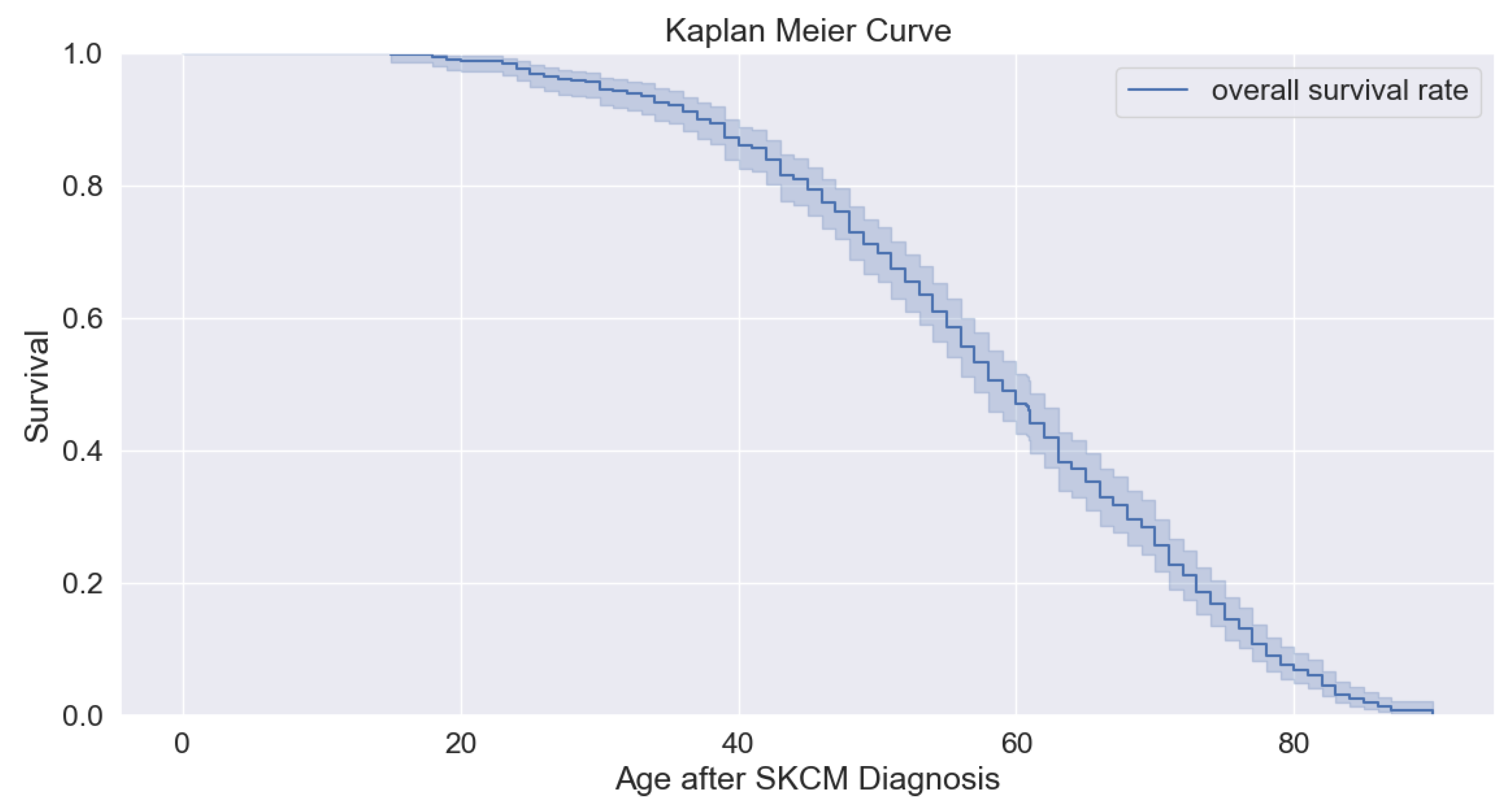
4.1. Survival Analysis Clinical Endpoint
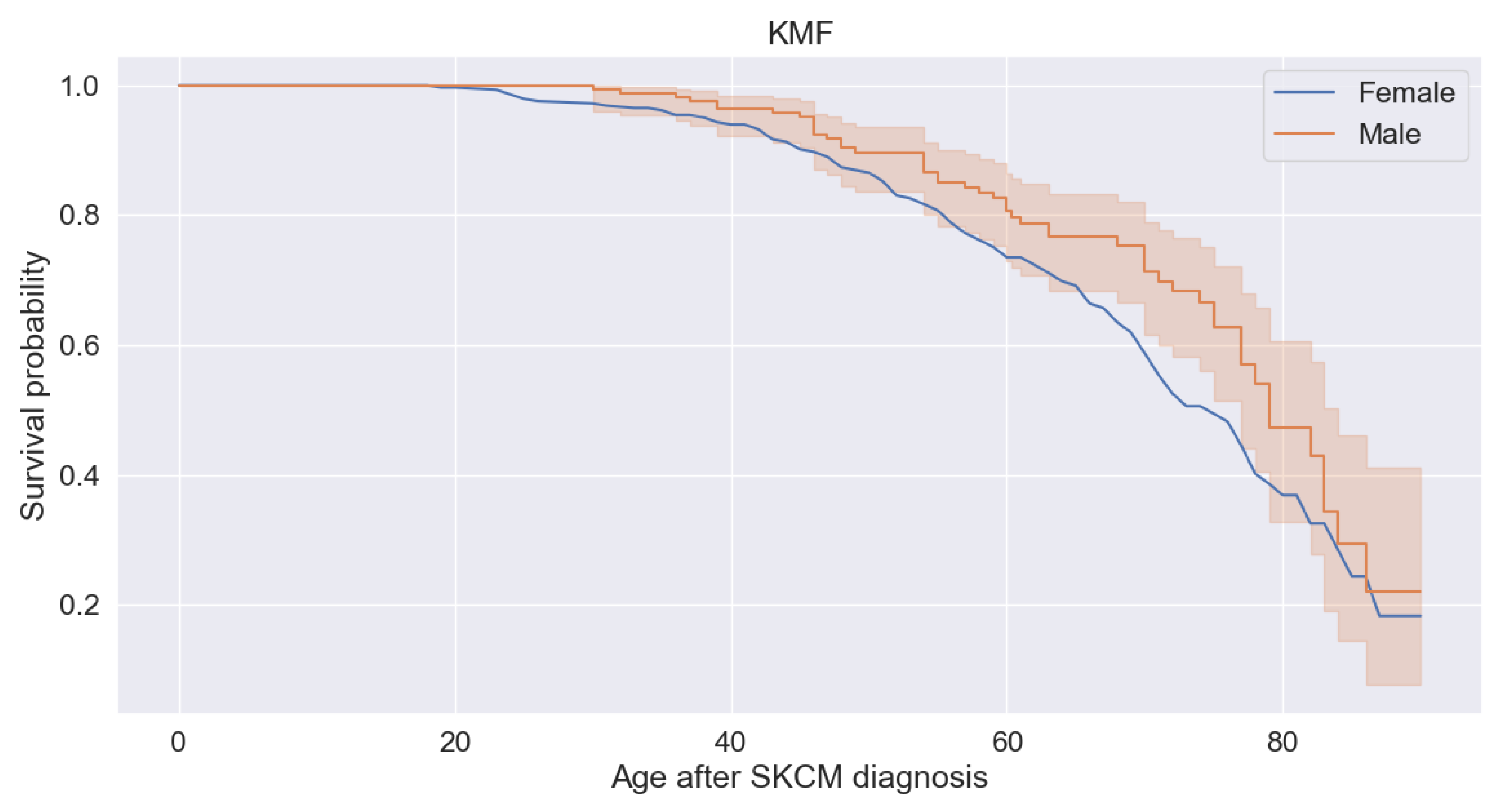
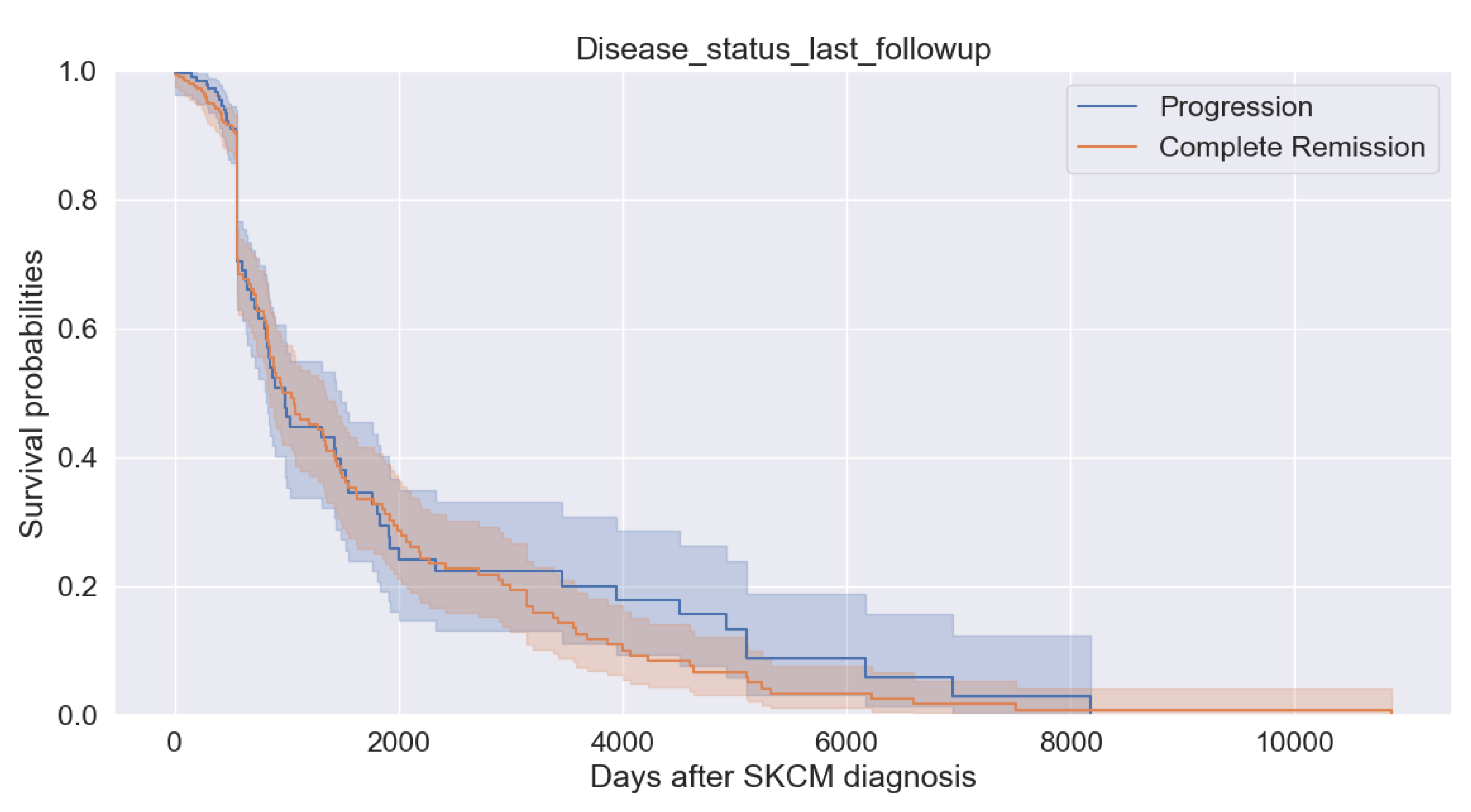
4.1.1. Kaplan–Meier Estimator
4.1.2. Cox Proportional Hazards Regression Model
- d represents survival time;
- represents the hazard function determined by a set of factors, i.e., ;
- defines the baseline hazard function representing event probability when all covariates are zero. Hazard value equals 1 when all are zero. The model assumes a parametric form for covariates’ effect on hazard without baseline assumptions;
- represents partial hazard as a time-invariant scalar factor that increases or decreases baseline hazard like the intercept in ordinary regression;
- The coefficients measure the impact of covariates on a subject’s hazard. The sign of the coefficient b affects the baseline hazard. A positive sign indicates higher risk, whereas a negative sign indicates lower risk. The magnitude of the coefficient b is estimated by maximizing partial likelihood. It assumes a proportional rate ratio throughout the study period, offering increased flexibility. This model can handle right-censored data but not left-censored or interval-censored data directly. The Cox model accepts the following three assumptions:
- 1.
- A constant hazard ratio;
- 2.
- The multiplicativity of explanatory variables;
- 3.
- The independent failure times for individual subjects.
4.1.3. ML-Based Ensemble Methods
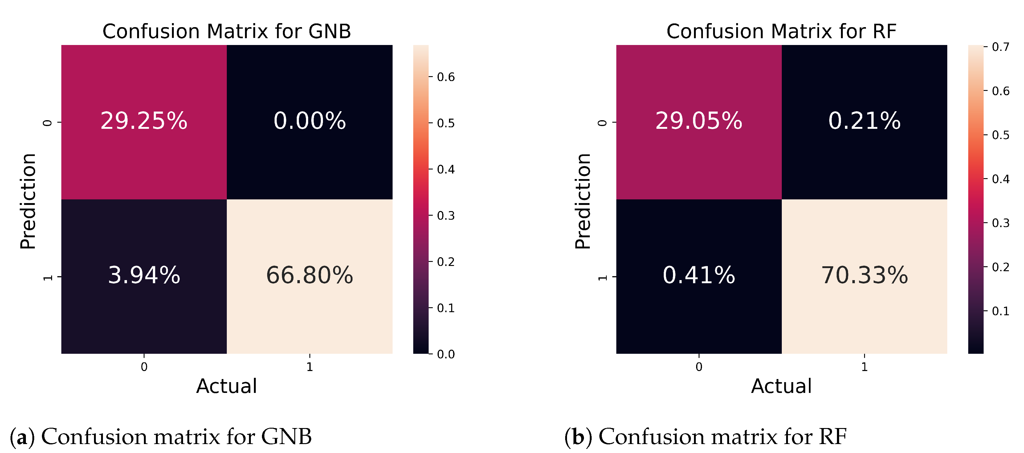
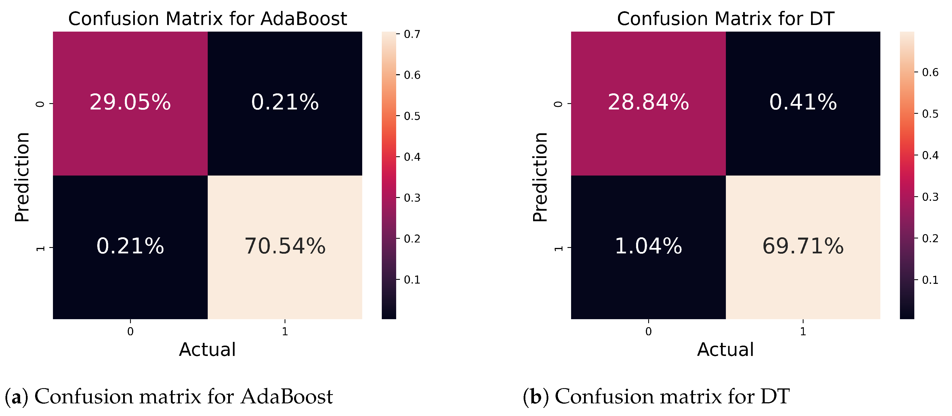
4.2. Comparative Study
4.3. Baseline Classifiers Standard Error
4.4. Discussion
5. Conclusions
Future Work
Author Contributions
Funding
Informed Consent Statement
Data Availability Statement
Conflicts of Interest
References
- Wang, X.; Xiong, H.; Liang, D.; Chen, Z.; Li, X.; Zhang, K. The role of SRGN in the survival and immune infiltrates of skin cutaneous melanoma (SKCM) and SKCM-metastasis patients. BMC Cancer 2020, 20, 378. [Google Scholar] [CrossRef] [PubMed]
- Ervik, F.; Ferlay, J.; Mery, L.; Soerjomataram, I.; Bray, F. Cancer Today; International Agency for Research on Cancer: Lyon, France, 2017. [Google Scholar]
- World Health Organization. World Health Statistics; Visual Summary; World Health Organization: Geneva, Switzerland, 2023. [Google Scholar]
- Naik, P.P. Cutaneous malignant melanoma: A review of early diagnosis and management. World J. Oncol. 2021, 12, 7. [Google Scholar] [CrossRef] [PubMed]
- Carr, S.; Smith, C.; Wernberg, J. Epidemiology and risk factors of melanoma. Surg. Clin. 2020, 100, 1–12. [Google Scholar] [CrossRef] [PubMed]
- Switzer, B.; Puzanov, I.; Skitzki, J.J.; Hamad, L.; Ernstoff, M.S. Managing metastatic melanoma in 2022: A clinical review. JCO Oncol. Pract. 2022, 18, 335–351. [Google Scholar] [CrossRef] [PubMed]
- Wu, Y.; Chen, B.; Zeng, A.; Pan, D.; Wang, R.; Zhao, S. Skin cancer classification with deep learning: A systematic review. Front. Oncol. 2022, 12, 893972. [Google Scholar] [CrossRef] [PubMed]
- Leiter, U.; Keim, U.; Garbe, C. Epidemiology of skin cancer: Update 2019. In Sunlight, Vitamin D and Skin Cancer; Springer: New York, NY, USA, 2020; pp. 123–139. [Google Scholar]
- Tang, Y.; Feng, H.; Zhang, L.; Qu, C.; Li, J.; Deng, X.; Zhong, S.; Yang, J.; Deng, X.; Zeng, X.; et al. A novel prognostic model for cutaneous melanoma based on an immune-related gene signature and clinical variables. Sci. Rep. 2022, 12, 20374. [Google Scholar] [CrossRef] [PubMed]
- Cozzolino, C.; Buja, A.; Rugge, M.; Miatton, A.; Zorzi, M.; Vecchiato, A.; Del Fiore, P.; Tropea, S.; Brazzale, A.; Damiani, G.; et al. Machine learning to predict overall short-term mortality in cutaneous melanoma. Discov. Oncol. 2023, 14, 13. [Google Scholar] [CrossRef]
- Dildar, M.; Akram, S.; Irfan, M.; Khan, H.U.; Ramzan, M.; Mahmood, A.R.; Alsaiari, S.A.; Saeed, A.H.M.; Alraddadi, M.O.; Mahnashi, M.H. Skin cancer detection: A review using deep learning techniques. Int. J. Environ. Res. Public Health 2021, 18, 5479. [Google Scholar] [CrossRef]
- Son, H.M.; Jeon, W.; Kim, J.; Heo, C.Y.; Yoon, H.J.; Park, J.U.; Chung, T.M. AI-based localization and classification of skin disease with erythema. Sci. Rep. 2021, 11, 5350. [Google Scholar] [CrossRef]
- Verma, A.K.; Pal, S.; Kumar, S. Comparison of skin disease prediction by feature selection using ensemble data mining techniques. Inform. Med. Unlocked 2019, 16, 100202. [Google Scholar] [CrossRef]
- Guo, P.; Xue, Z.; Mtema, Z.; Yeates, K.; Ginsburg, O.; Demarco, M.; Long, L.R.; Schiffman, M.; Antani, S. Ensemble deep learning for cervix image selection toward improving reliability in automated cervical precancer screening. Diagnostics 2020, 10, 451. [Google Scholar] [CrossRef] [PubMed]
- Mamun, M.; Farjana, A.; Al Mamun, M.; Ahammed, M.S. Lung cancer prediction model using ensemble learning techniques and a systematic review analysis. In Proceedings of the 2022 IEEE World AI IoT Congress (AIIoT), Seattle, WA, USA, 6–9 June 2022; pp. 187–193. [Google Scholar]
- ICGC Data Portal—Skin Cutaneous Melanoma (SKCM)—US Project. Available online: https://dcc.icgc.org/releases/current/Projects/SKCM-US (accessed on 27 November 2023).
- Aamir, S.; Rahim, A.; Aamir, Z.; Abbasi, S.F.; Khan, M.S.; Alhaisoni, M.; Khan, M.A.; Khan, K.; Ahmad, J. Predicting breast cancer leveraging supervised machine learning techniques. Comput. Math. Methods Med. 2022, 2022, 5869529. [Google Scholar] [CrossRef] [PubMed]
- Shah, S.A.; Tahir, A.; Ahmad, J.; Zahid, A.; Pervaiz, H.; Shah, S.Y.; Ashleibta, A.M.A.; Hasanali, A.; Khattak, S.; Abbasi, Q.H. Sensor fusion for identification of freezing of gait episodes using Wi-Fi and radar imaging. IEEE Sens. J. 2020, 20, 14410–14422. [Google Scholar] [CrossRef]
- Magsi, A.H.; Mohsan, S.A.H.; Muhammad, G.; Abbasi, S. A Machine Learning-Based Interest Flooding Attack Detection System in Vehicular Named Data Networking. Electronics 2023, 12, 3870. [Google Scholar] [CrossRef]
- Magsi, A.H.; Ghulam, A.; Memon, S.; Javeed, K.; Alhussein, M.; Rida, I. A Machine Learning-Based Attack Detection and Prevention System in Vehicular Named Data Networking. Comput. Mater. Contin. 2023, 77, 1445–1465. [Google Scholar] [CrossRef]
- Trang, K.; Nguyen, H.A.; TonThat, L.; Do, H.N.; Vuong, B.Q. An Ensemble Voting Method of Pre-Trained Deep Learning Models for Skin Disease Identification. In Proceedings of the 2022 IEEE International Conference on Cybernetics and Computational Intelligence (CyberneticsCom), Malang, Indonesia, 16–18 June 2022; pp. 445–450. [Google Scholar]
- Verma, A.K.; Pal, S.; Tiwari, B. Skin disease prediction using ensemble methods and a new hybrid feature selection technique. Iran J. Comput. Sci. 2020, 3, 207–216. [Google Scholar] [CrossRef]
- Thanka, M.R.; Edwin, E.B.; Ebenezer, V.; Sagayam, K.M.; Reddy, B.J.; Günerhan, H.; Emadifar, H. A hybrid approach for melanoma classification using ensemble machine learning techniques with deep transfer learning. Comput. Methods Programs Biomed. Update 2023, 3, 100103. [Google Scholar]
- Bradburn, M.J.; Clark, T.G.; Love, S.B.; Altman, D.G. Survival analysis part II: Multivariate data analysis—An introduction to concepts and methods. Br. J. Cancer 2003, 89, 431–436. [Google Scholar] [CrossRef]
- Shorfuzzaman, M. An explainable stacked ensemble of deep learning models for improved melanoma skin cancer detection. Multimed. Syst. 2022, 28, 1309–1323. [Google Scholar] [CrossRef]
- Alam, T.M.; Shaukat, K.; Khan, W.A.; Hameed, I.A.; Almuqren, L.A.; Raza, M.A.; Aslam, M.; Luo, S. An efficient deep learning-based skin cancer classifier for an imbalanced dataset. Diagnostics 2022, 12, 2115. [Google Scholar] [CrossRef]
- Alwakid, G.; Gouda, W.; Humayun, M.; Sama, N.U. Melanoma detection using deep learning-based classifications. Healthcare 2022, 10, 2481. [Google Scholar] [CrossRef] [PubMed]
- Ali, M.S.; Miah, M.S.; Haque, J.; Rahman, M.M.; Islam, M.K. An enhanced technique of skin cancer classification using deep convolutional neural network with transfer learning models. Mach. Learn. Appl. 2021, 5, 100036. [Google Scholar] [CrossRef]
- Naeem, A.; Anees, T.; Fiza, M.; Naqvi, R.A.; Lee, S.W. SCDNet: A Deep Learning-Based Framework for the Multiclassification of Skin Cancer Using Dermoscopy Images. Sensors 2022, 22, 5652. [Google Scholar] [CrossRef] [PubMed]
- Huang, M.; Zhang, Y.; Ou, X.; Wang, C.; Wang, X.; Qin, B.; Zhang, Q.; Yu, J.; Zhang, J.; Yu, J.; et al. m5C-related signatures for predicting prognosis in cutaneous melanoma with machine learning. J. Oncol. 2021, 2021, 6173206. [Google Scholar] [CrossRef] [PubMed]
- Agrahari, P.; Agrawal, A.; Subhashini, N. Skin cancer detection using deep learning. In Futuristic Communication and Network Technologies: Select Proceedings of VICFCNT 2020; Springer: Berlin/Heidelberg, Germany, 2022; pp. 179–190. [Google Scholar]
- Wang, Y.; Singh, L. Analyzing the impact of missing values and selection bias on fairness. Int. J. Data Sci. Anal. 2021, 12, 101–119. [Google Scholar] [CrossRef]
- Mera-Gaona, M.; Neumann, U.; Vargas-Canas, R.; López, D.M. Evaluating the impact of multivariate imputation by MICE in feature selection. PLoS ONE 2021, 16, e0254720. [Google Scholar] [CrossRef] [PubMed]
- Hambali, M.A.; Oladele, T.O.; Adewole, K.S. Microarray cancer feature selection: Review, challenges and research directions. Int. J. Cogn. Comput. Eng. 2020, 1, 78–97. [Google Scholar] [CrossRef]
- He, Z.; Li, L.; Huang, Z.; Situ, H. Quantum-enhanced feature selection with forward selection and backward elimination. Quantum Inf. Process. 2018, 17, 154. [Google Scholar] [CrossRef]
- Chowdhury, M.Z.I.; Turin, T.C. Variable selection strategies and its importance in clinical prediction modelling. Fam. Med. Community Health 2020, 8, e000262. [Google Scholar] [CrossRef]
- Abd ElHafeez, S.; D’Arrigo, G.; Leonardis, D.; Fusaro, M.; Tripepi, G.; Roumeliotis, S. Methods to analyze time-to-event data: The Cox regression analysis. Oxidative Med. Cell. Longev. 2021, 2021, 1302811. [Google Scholar] [CrossRef]
- Nikulin, M.; Wu, H.D. The Cox Model and Its Applications; Springer: Berlin/Heidelberg, Germany, 2016. [Google Scholar]


| Ref. | Method | Study Area | Dataset | Results | Limitations |
|---|---|---|---|---|---|
| [25] | A CNN-based melanoma skin cancer detection | Skin cancer | Open access dataset | 95% | No multi-omics exploited |
| [26] | DL-based skin cancer detection system | Skin cancer | HAM 10000 | 91% | The accuracy of proposed study is poor |
| [27] | DL-based melanoma detection | Skin cancer | HAM 10000 | 86% | Various models and datasets call for different hyperparameter settings |
| [28] | CNN-based skin cancer detection | Skin cancer | HAM 10000 | 91.93% | The limited size of the datasets employed in this study may have led to local optimizations |
| [29] | A DL-based framework for the multi-classification of skin cancer using dermoscopy images | Skin cancer | ISIC 2019 | 92% | Lower accuracy |
| [9] | Immune cell infiltration pattern of CM | SKCM | - | - | The study does not utilize any ML/DL algorithms to show a better performance |
| [10] | DL-based short-term survival of cutaneous malignant melanoma (CMM) | SKCM | RNA-seq | 91% | Lower accuracy |
| [30] | The mRNA expressions of m5C regulators in colorectal cancer tissues | Various cancer types | RNA-seq | - | Performance metrics were not evaluated |
| [31] | DL-based multiclass skin cancer diagnosis | Skin cancer | HAM 10000 ISIC | 96.26% | The accuracy of this study is lower |
| Notation | Description |
|---|---|
| A | Input set of features for backward selection |
| Initialize the function with a full set of features | |
| w | Subset of output features |
| r | A finite set of input features |
| Output set of features | |
| Selection criteria function | |
| Subset of output features | |
| L | The desired set of features |
| m | A finite set of output features |
| X | Input set features for forward selection |
| Initialize the function with an empty set | |
| Selection criteria function | |
| h | The desired set of features |
| Output set of features | |
| Subset of output features | |
| t | Size of a subset of output features |
| The likelihood of the event occurred | |
| Time at which event occurred or did not occur | |
| Y | Random duration of survival function |
| Number of patients | |
| Number of incidents | |
| Life risk at a time | |
| d | Survival time |
| Hazard function | |
| Set of factors | |
| Baseline hazard function | |
| Measure of the impact of covariates on a subject’s hazard |
| Class | Records per Class | Features |
|---|---|---|
| Donor | 471 | 9 |
| Simple_somatic_mutation | 1,048,576 | 12 |
| Copy-number_soamtic_mutation | 377,735 | 3 |
| Mirna _seq | 369,409 | 5 |
| Specimen | 947 | 2 |
| Total Records | 1,797,138 | 31 |
| Covariate | Coef | Exp (Coef) | Se (Coef) | Coef Lower (95%) | Coef Upper (95%) | Exp Coef Lower (95%) | Exp Coef Upper (95%) | z | p | log2 (p) |
|---|---|---|---|---|---|---|---|---|---|---|
| Sex | 0.02 | 1.02 | 0.10 | −0.17 | 0.21 | 0.84 | 1.23 | 1.02 | 0.10 | −0.17 |
| Status | −0.12 | 0.98 | 0.19 | −0.39 | 0.35 | 0.68 | 1.41 | 0.98 | 0.19 | −0.39 |
| Disease status last followup | −0.00 | 0.98 | 0.10 | −0.21 | 0.17 | 0.81 | 1.18 | 0.98 | 0.10 | −0.21 |
| Age at last followup | −0.50 | 0.61 | 0.02 | −0.55 | −0.46 | 0.58 | 0.63 | 0.61 | 0.02 | −0.55 |
| Diagnosis | −0.00 | 1.00 | 0.00 | −0.01 | 0.00 | 0.99 | 1.00 | 1.00 | 0.00 | −0.01 |
| Interval | 0.49 | 1.64 | 0.03 | 0.44 | 0.54 | 1.56 | 1.72 | 1.64 | 0.03 | 0.44 |
| Feature Selection Methods | Score |
|---|---|
| Backward Feature Elimination | 0.99993 |
| Forward Feature Elimination | 0.99988 |
| Recursive Feature Elimination | 0.99400 |
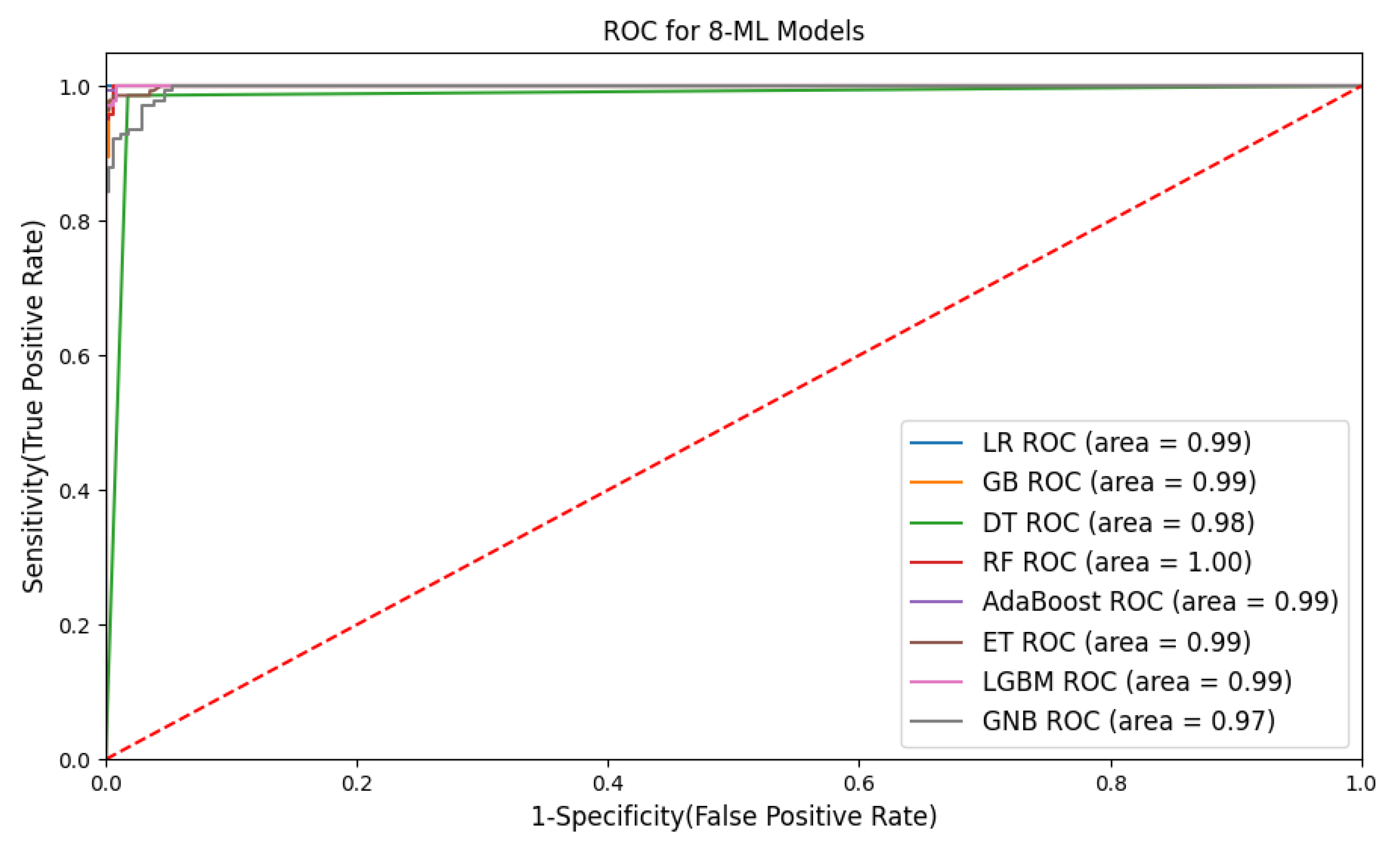
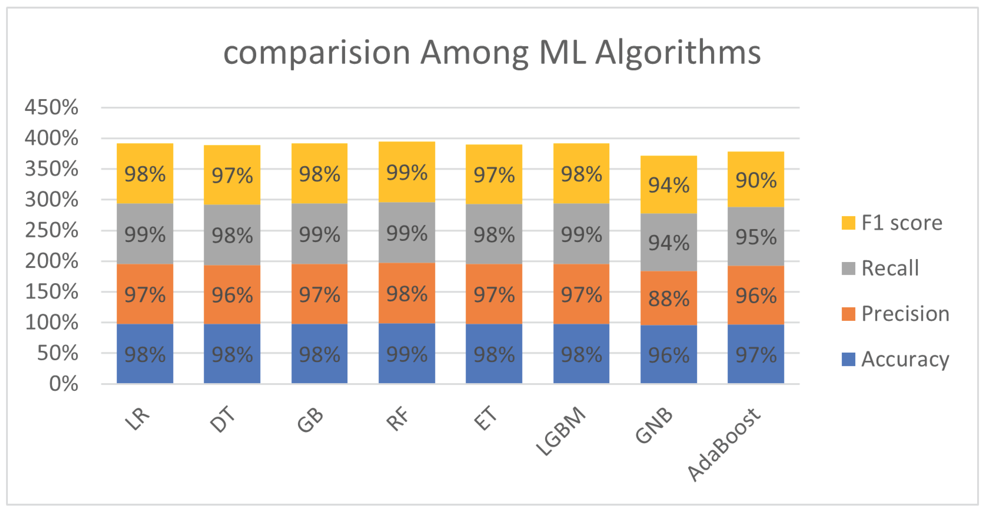
| ML Algorithms | Accuracy | Precision | Recall | F1 Score |
|---|---|---|---|---|
| LR | 98% | 97% | 99% | 98% |
| DT | 98% | 96% | 98% | 97% |
| GB | 98% | 97% | 99% | 98% |
| RF | 99% | 98% | 99% | 99% |
| ET | 98% | 97% | 98% | 97% |
| AdaBoost | 97% | 96% | 95% | 90% |
| LGBM | 98% | 97% | 99% | 98% |
| GNB | 96% | 88% | 94% | 94% |
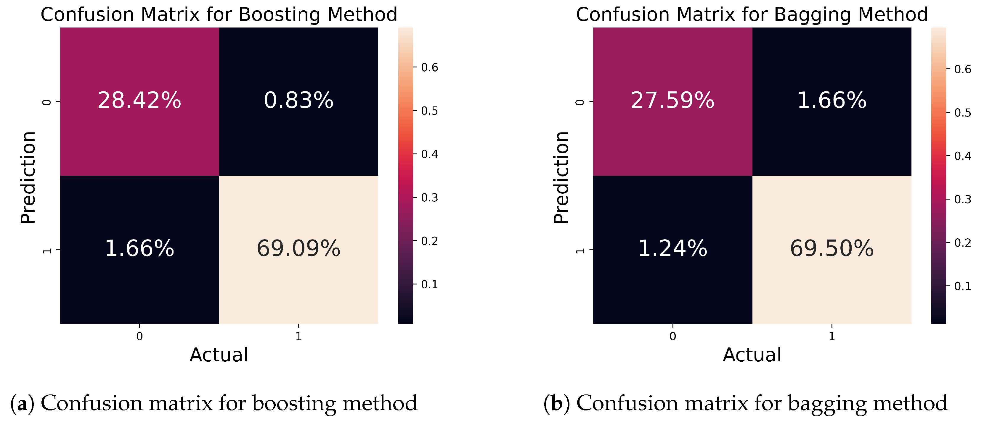
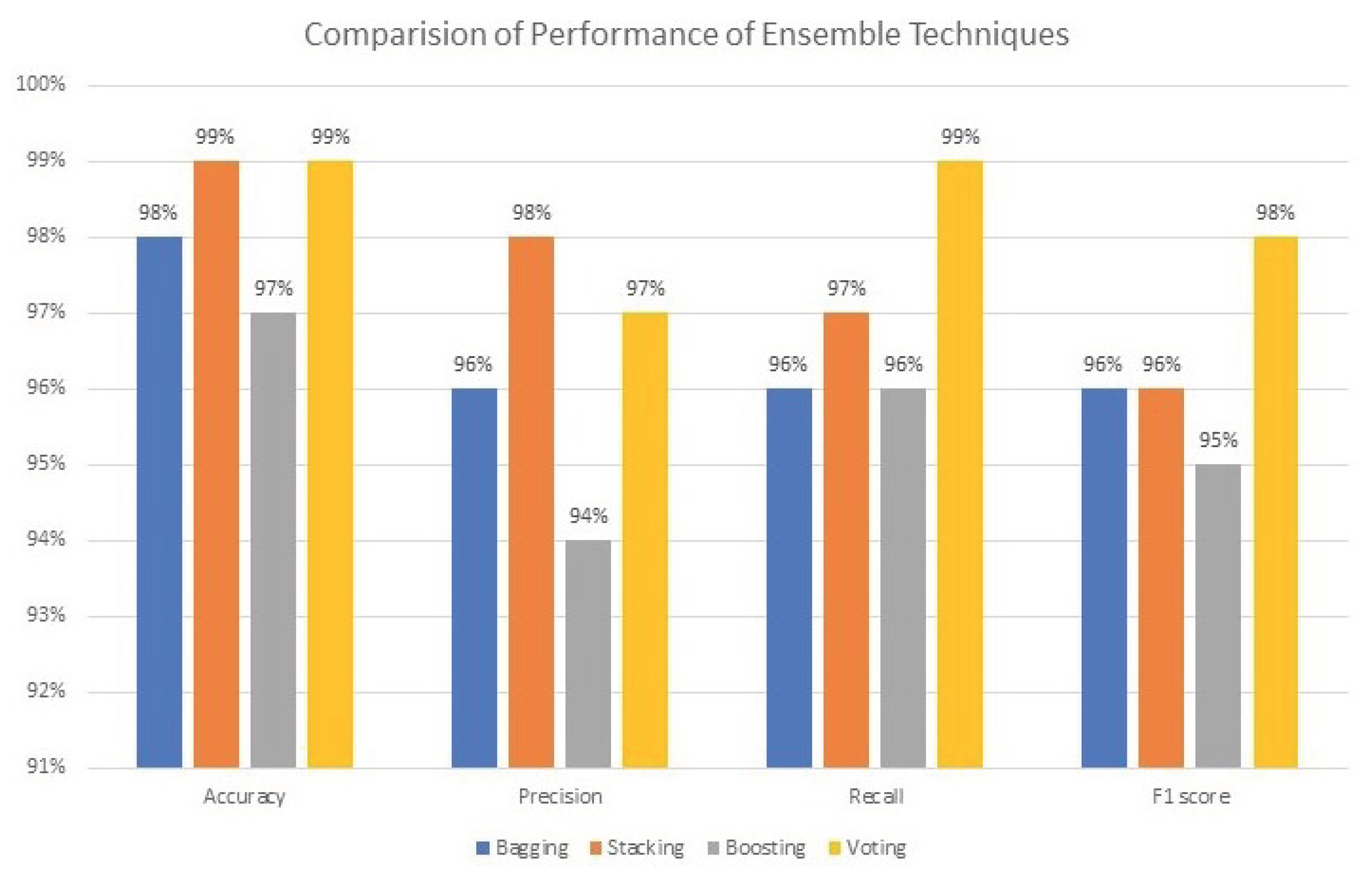
| Ensemble Methods | Accuracy | Precision | Recall | F1 Score |
|---|---|---|---|---|
| Bagging | 98% | 96% | 96% | 96% |
| Stacking | 99% | 98% | 97% | 96% |
| Boosting | 97% | 94% | 96% | 95% |
| Voting | 99% | 97% | 99% | 98% |
| ML Classifiers | Accuracy | Precision | Recall | F1 Score |
|---|---|---|---|---|
| RF | 99% | 98% | 99% | 99% |
| GNB | 96% | 88% | 94% | 94% |
| LR | 98% | 97% | 99% | 98% |
| DT | 98% | 96% | 99% | 98% |
| GB | 98% | 97% | 99% | 98% |
| Adaboost | 97% | 96% | 95% | 90% |
| Extratree | 98% | 97% | 98% | 97% |
| LGBM | 98% | 97% | 99% | 98% |
| Bagging | 98% | 96% | 96% | 96% |
| Stacking | 99% | 98% | 97% | 96% |
| Boosting | 97% | 94% | 96% | 95% |
| Voting | 99% | 97% | 99% | 98% |
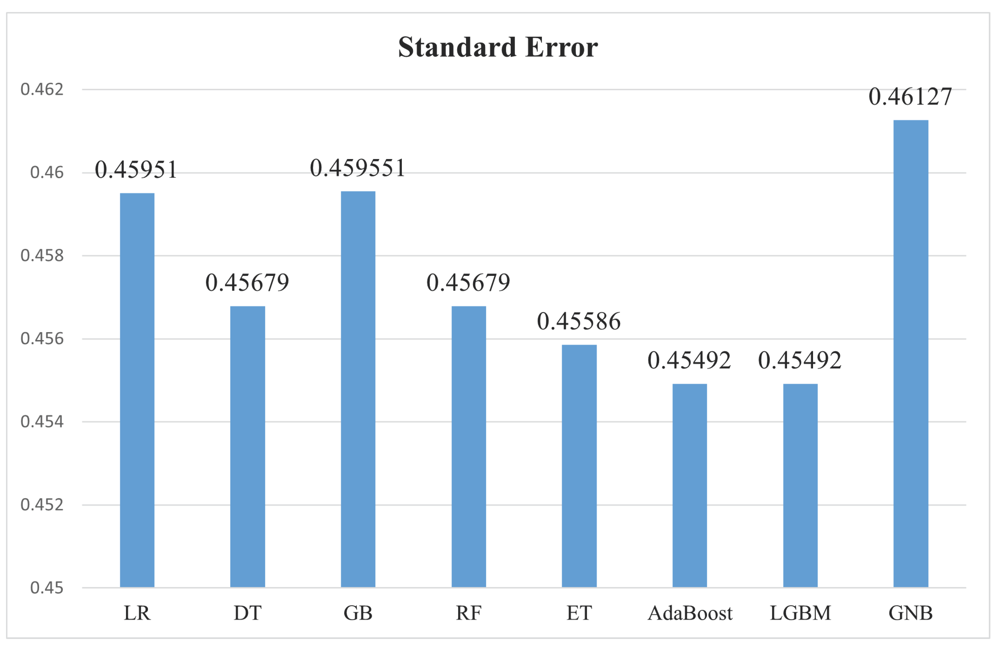
| Baseline Classifiers | Standard Error |
|---|---|
| LR | 0.45951 |
| DT | 0.45679 |
| GB | 0.459551 |
| RF | 0.45679 |
| ET | 0.45586 |
| AdaBoost | 0.45492 |
| LGBM | 0.45492 |
| GNB | 0.46127 |
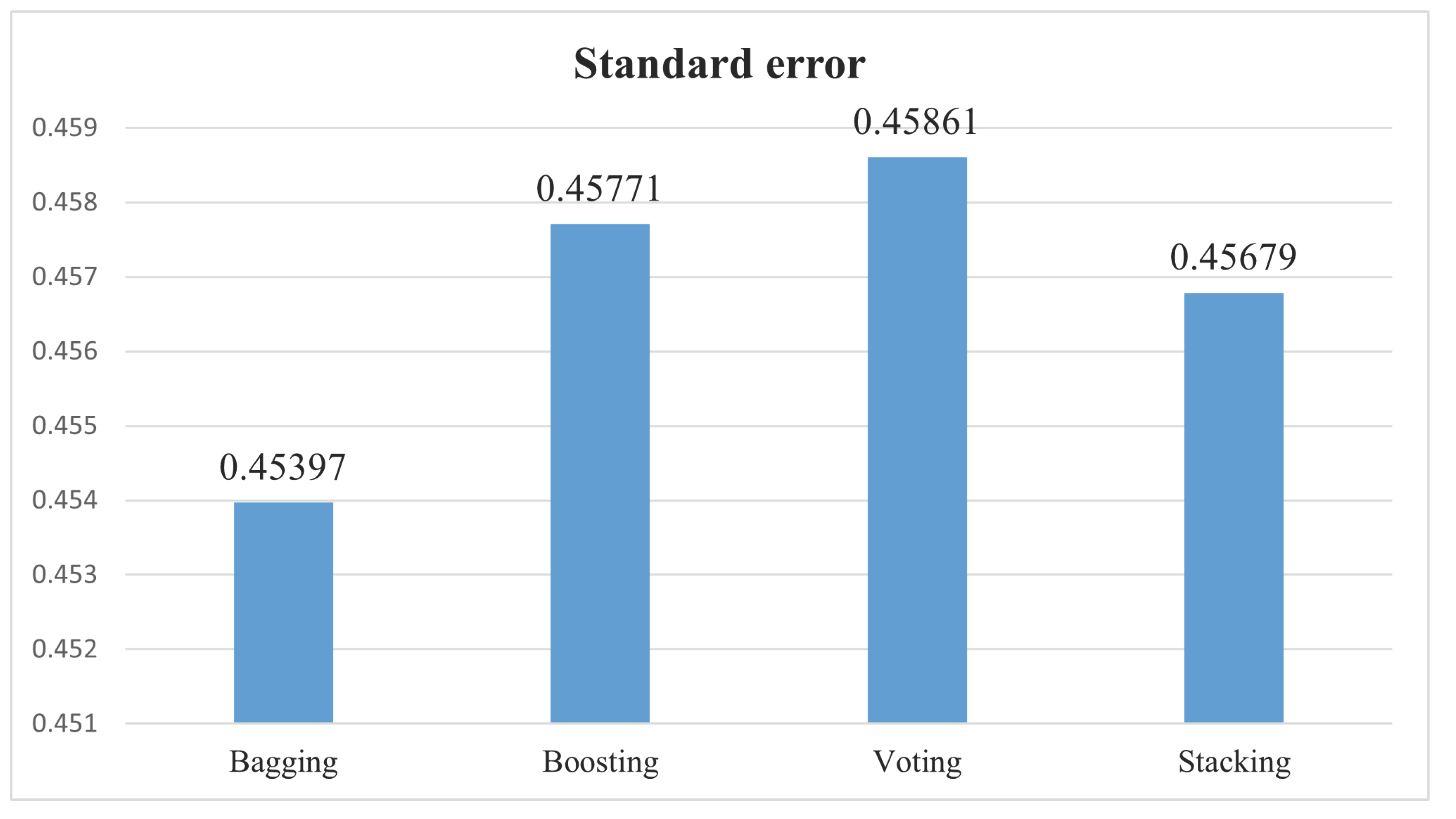
| Ensemble Methods | Standard Error |
|---|---|
| Bagging | 0.45397 |
| Boosting | 0.45771 |
| Voting | 0.45861 |
| Stacking | 0.45679 |
Disclaimer/Publisher’s Note: The statements, opinions and data contained in all publications are solely those of the individual author(s) and contributor(s) and not of MDPI and/or the editor(s). MDPI and/or the editor(s) disclaim responsibility for any injury to people or property resulting from any ideas, methods, instructions or products referred to in the content. |
© 2023 by the authors. Licensee MDPI, Basel, Switzerland. This article is an open access article distributed under the terms and conditions of the Creative Commons Attribution (CC BY) license (https://creativecommons.org/licenses/by/4.0/).
Share and Cite
Abbasi, E.Y.; Deng, Z.; Magsi, A.H.; Ali, Q.; Kumar, K.; Zubedi, A. Optimizing Skin Cancer Survival Prediction with Ensemble Techniques. Bioengineering 2024, 11, 43. https://doi.org/10.3390/bioengineering11010043
Abbasi EY, Deng Z, Magsi AH, Ali Q, Kumar K, Zubedi A. Optimizing Skin Cancer Survival Prediction with Ensemble Techniques. Bioengineering. 2024; 11(1):43. https://doi.org/10.3390/bioengineering11010043
Chicago/Turabian StyleAbbasi, Erum Yousef, Zhongliang Deng, Arif Hussain Magsi, Qasim Ali, Kamlesh Kumar, and Asma Zubedi. 2024. "Optimizing Skin Cancer Survival Prediction with Ensemble Techniques" Bioengineering 11, no. 1: 43. https://doi.org/10.3390/bioengineering11010043
APA StyleAbbasi, E. Y., Deng, Z., Magsi, A. H., Ali, Q., Kumar, K., & Zubedi, A. (2024). Optimizing Skin Cancer Survival Prediction with Ensemble Techniques. Bioengineering, 11(1), 43. https://doi.org/10.3390/bioengineering11010043