

Multiscale Homogenization Techniques for TPMS Foam Material for Biomedical Structural Applications


Abstract
1. Introduction
Lattice Materials for Tissue Engineering
- biocompatibility;
- biodegradability;
- mechanical properties to bear weight during the amelioration period;
- proper architecture in terms of porosity and pore sizes;
- sterilibility without loss of bioactivity;
- controlled deliverability of bioactive molecules or drugs;
2. Homogenization Techniques
2.1. Boundary Conditions
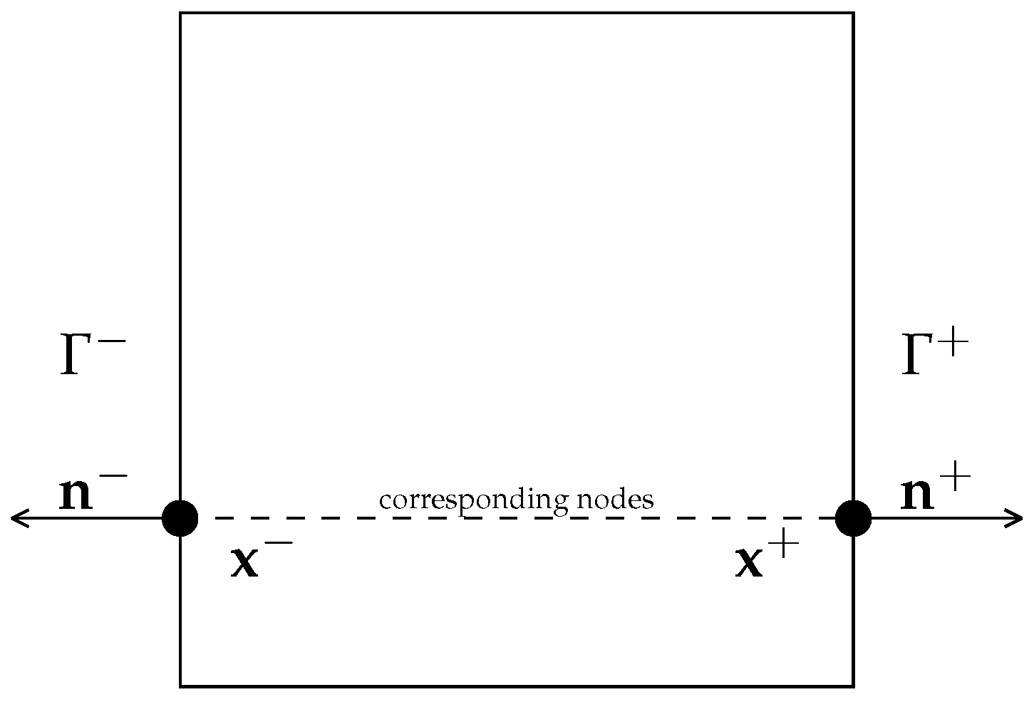
2.1.1. Periodic Boundary Conditions
2.1.2. Linear Displacement and Uniform Traction Boundary Condition
2.2. FE Homogenization
2.3. Mechanical Properties
Elastic Properties
2.4. Plastic Properties
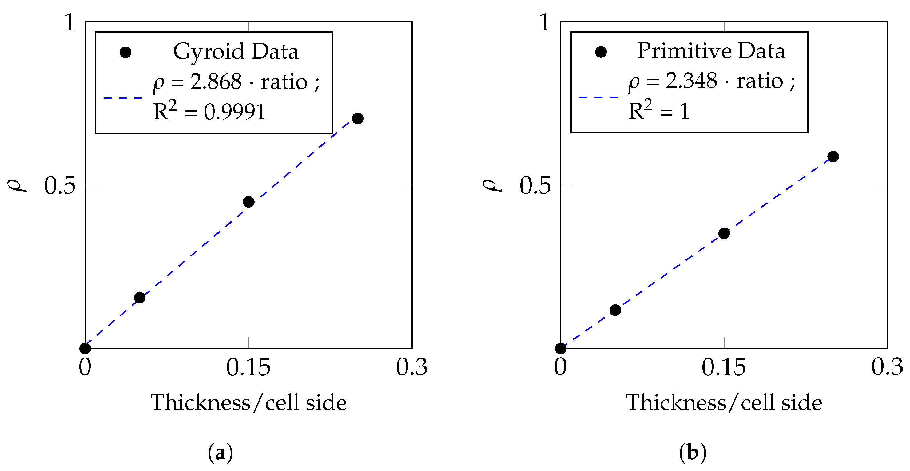
2.5. Scaling Laws
3. Materials and Methods
3.1. Materials
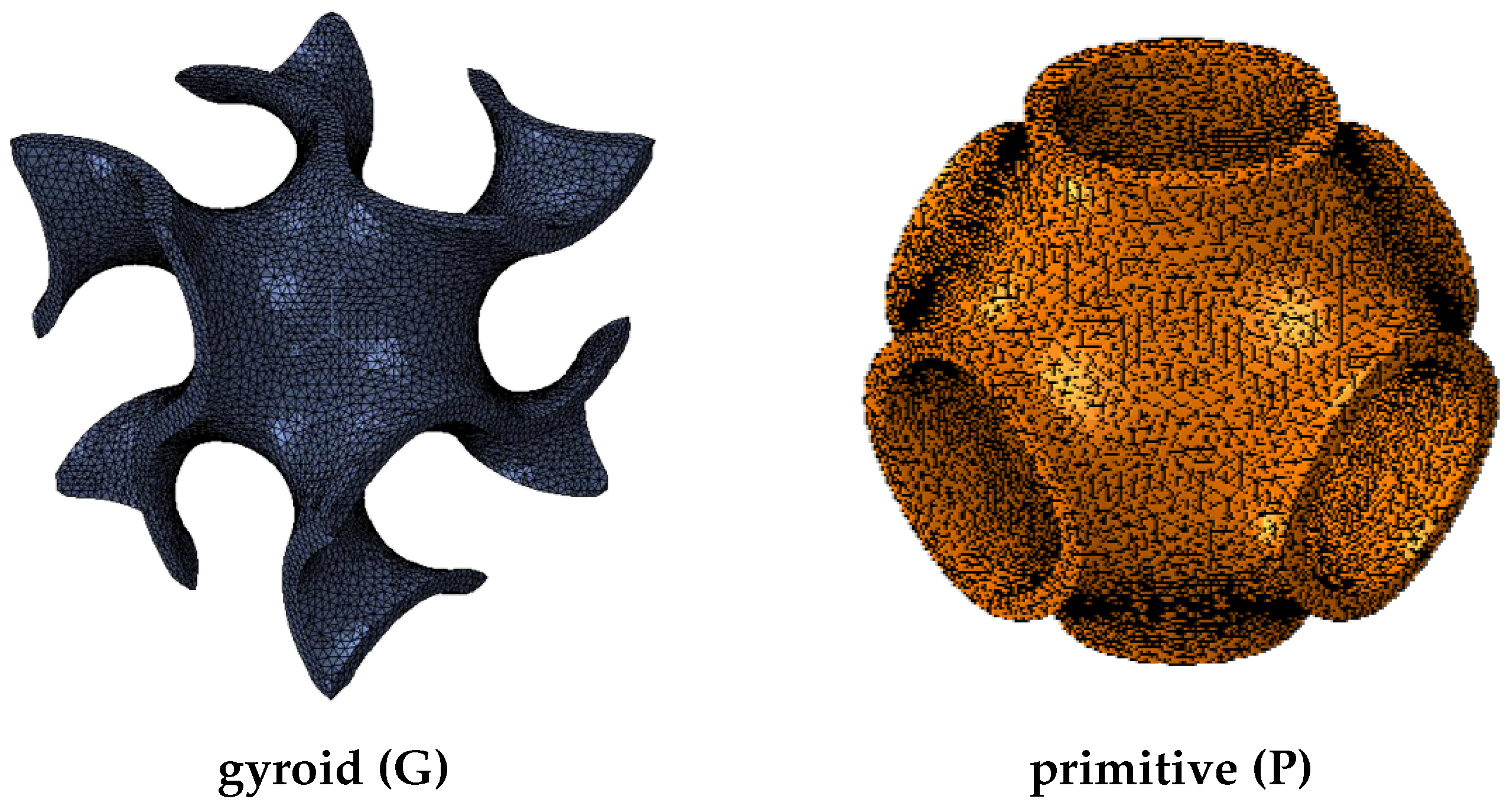
3.2. Models
3.3. Boundary Conditions
3.3.1. Periodic Boundary Conditions
3.3.2. Homogenization Boundary Conditions
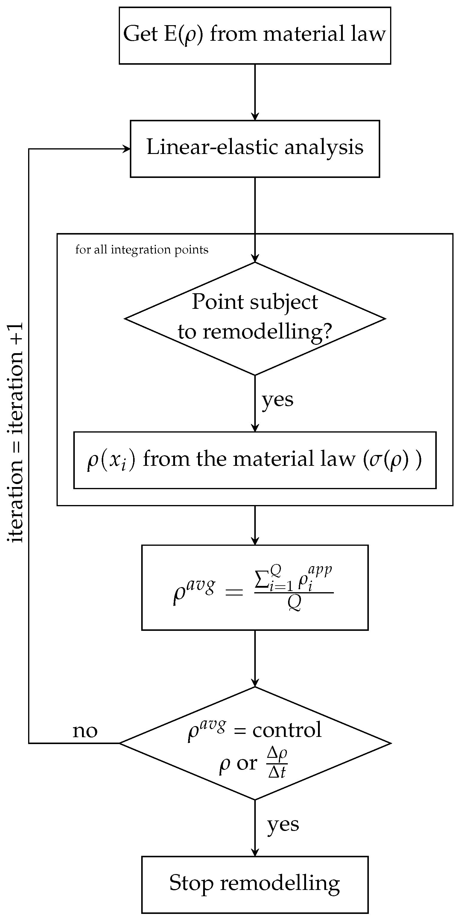
3.4. Bio-Inspired Remodelling Algorithm
3.5. Stress Shielding Evaluation
4. Results and Discussion
4.1. Topology Analysis
4.2. Elastic Properties
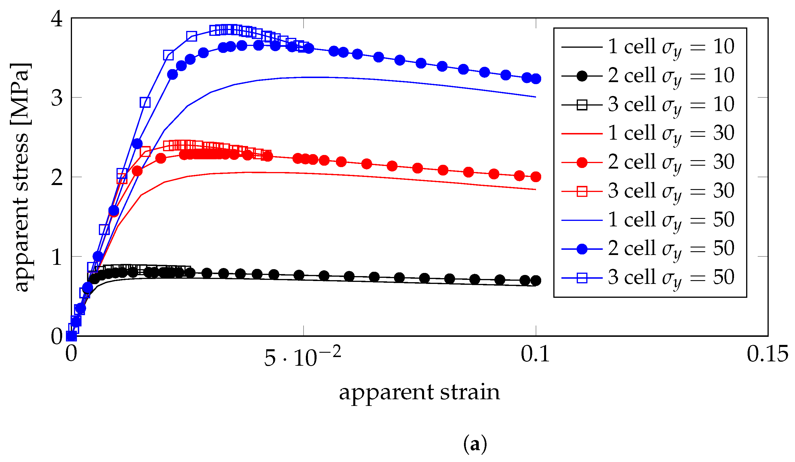
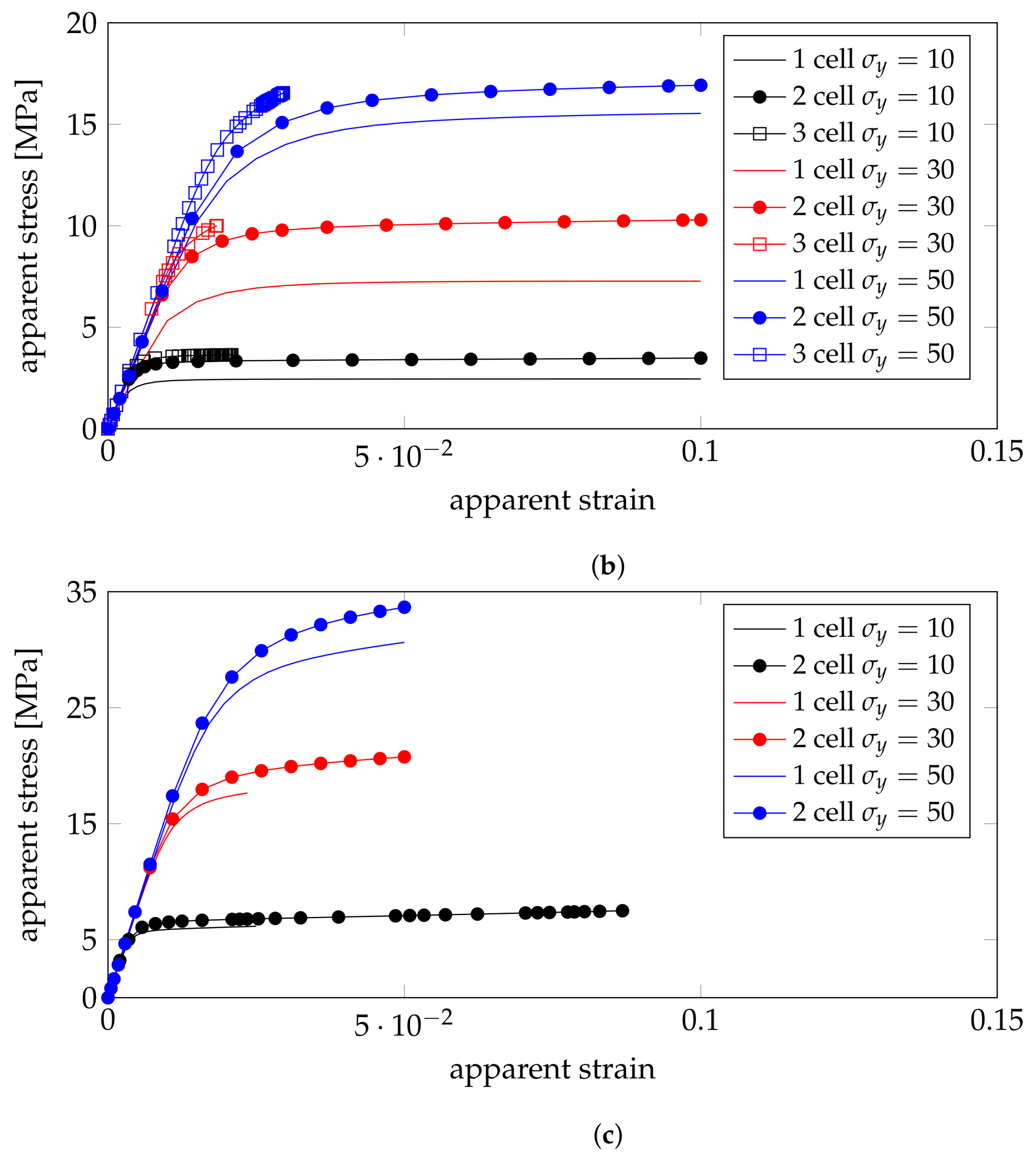
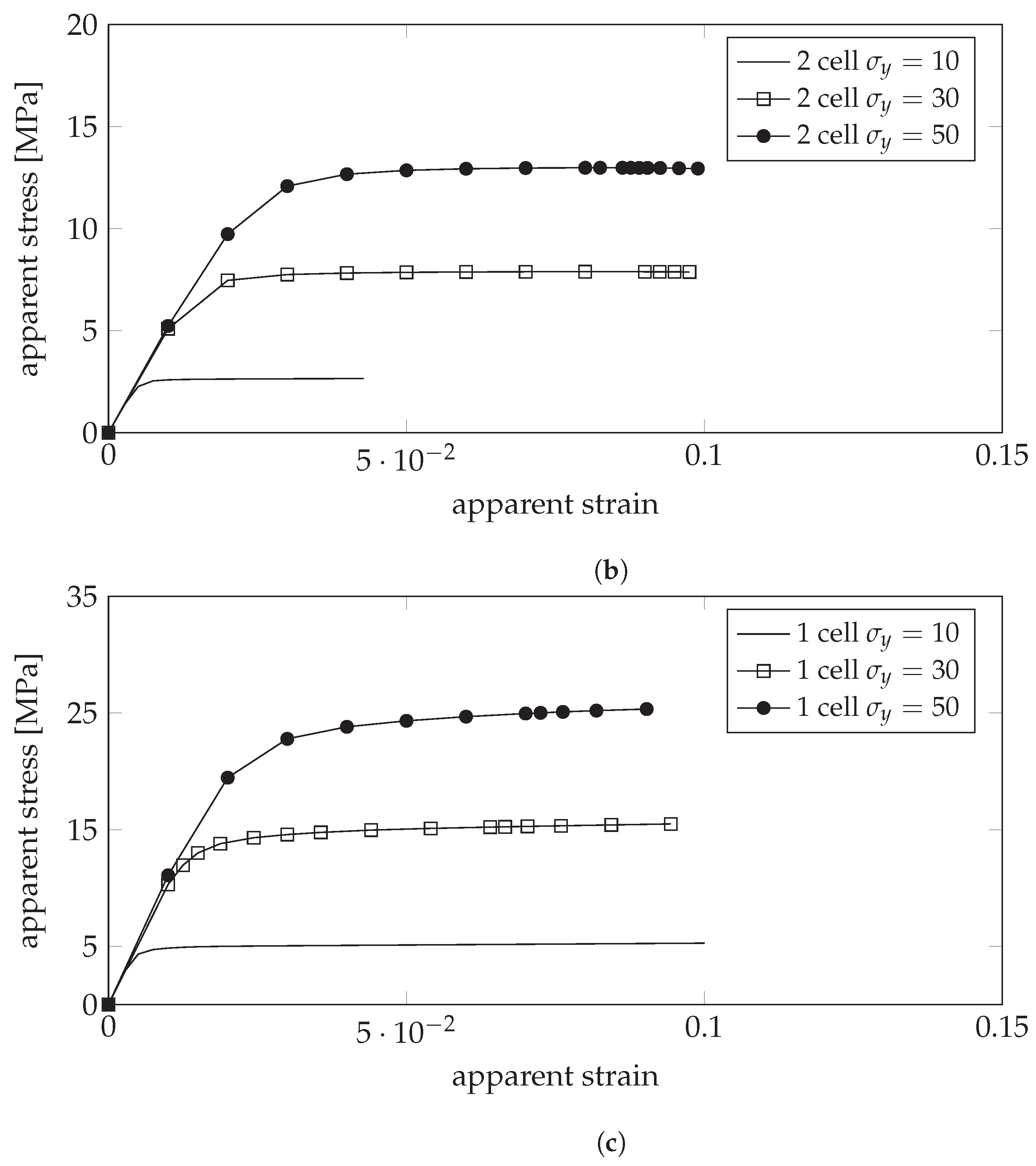
4.3. Plastic Properties
5. Discussion
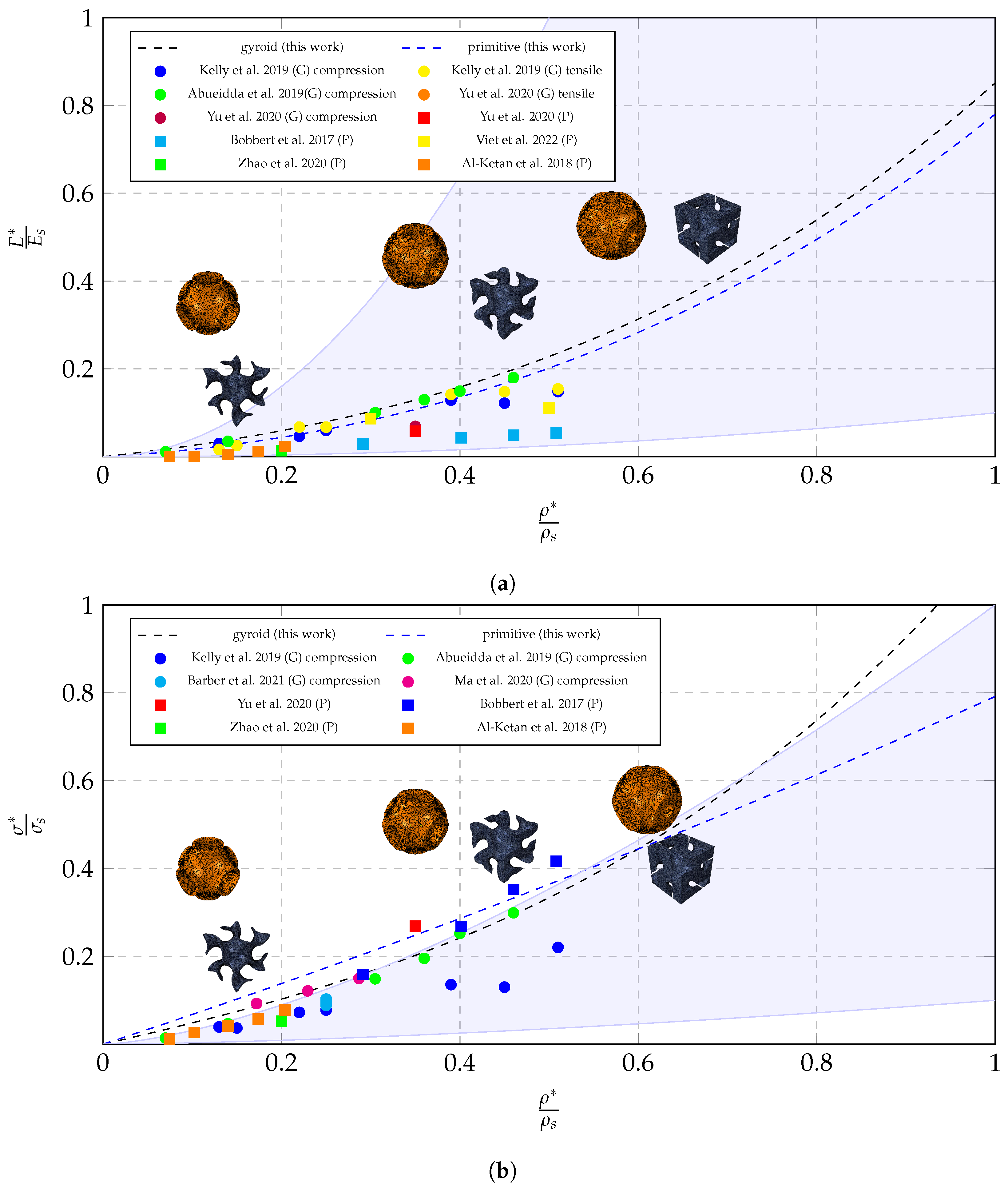
5.1. Material Law and Comparison to Literature Data
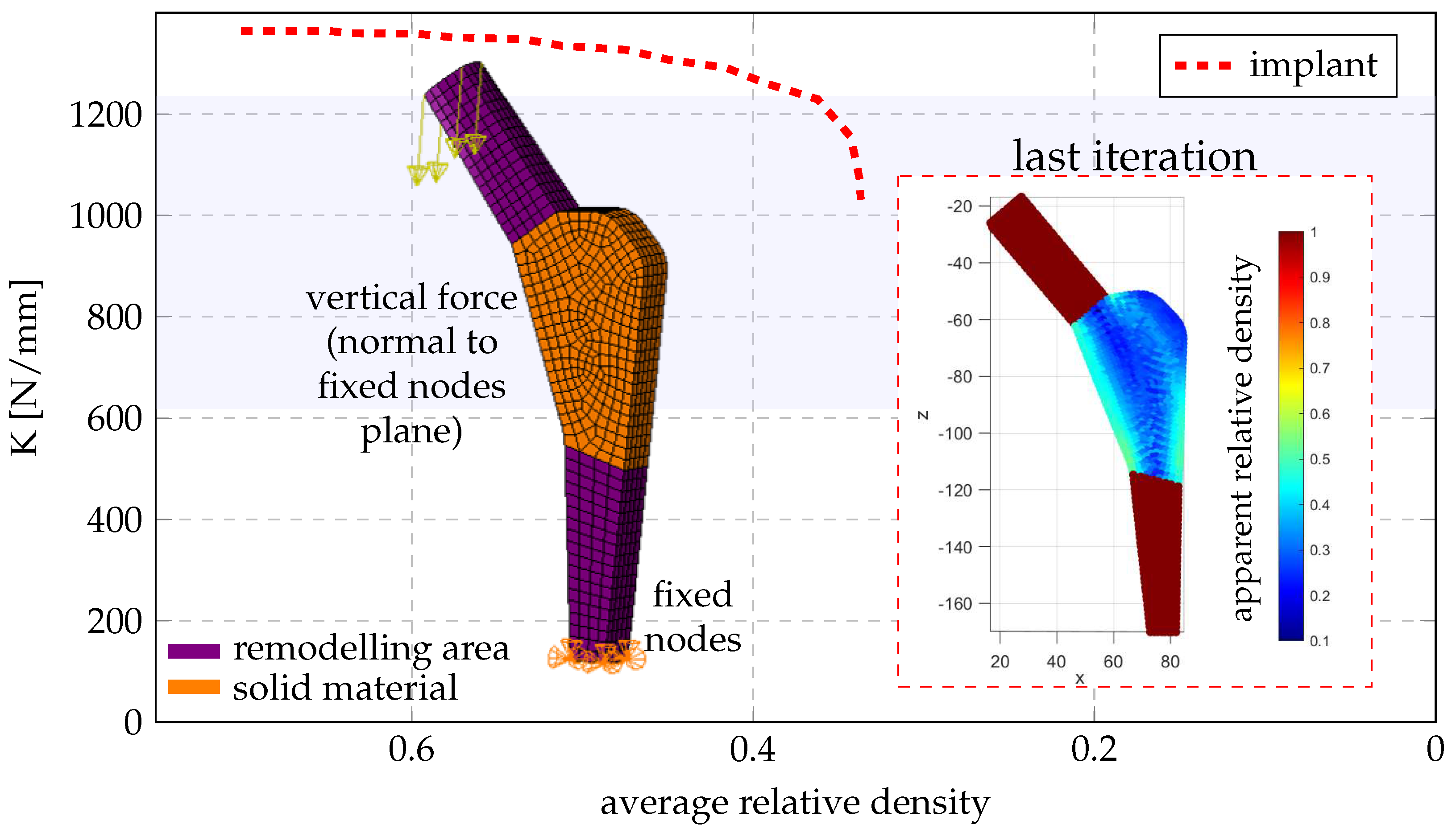
5.2. Study Case-Femoral Stem
Implant Model
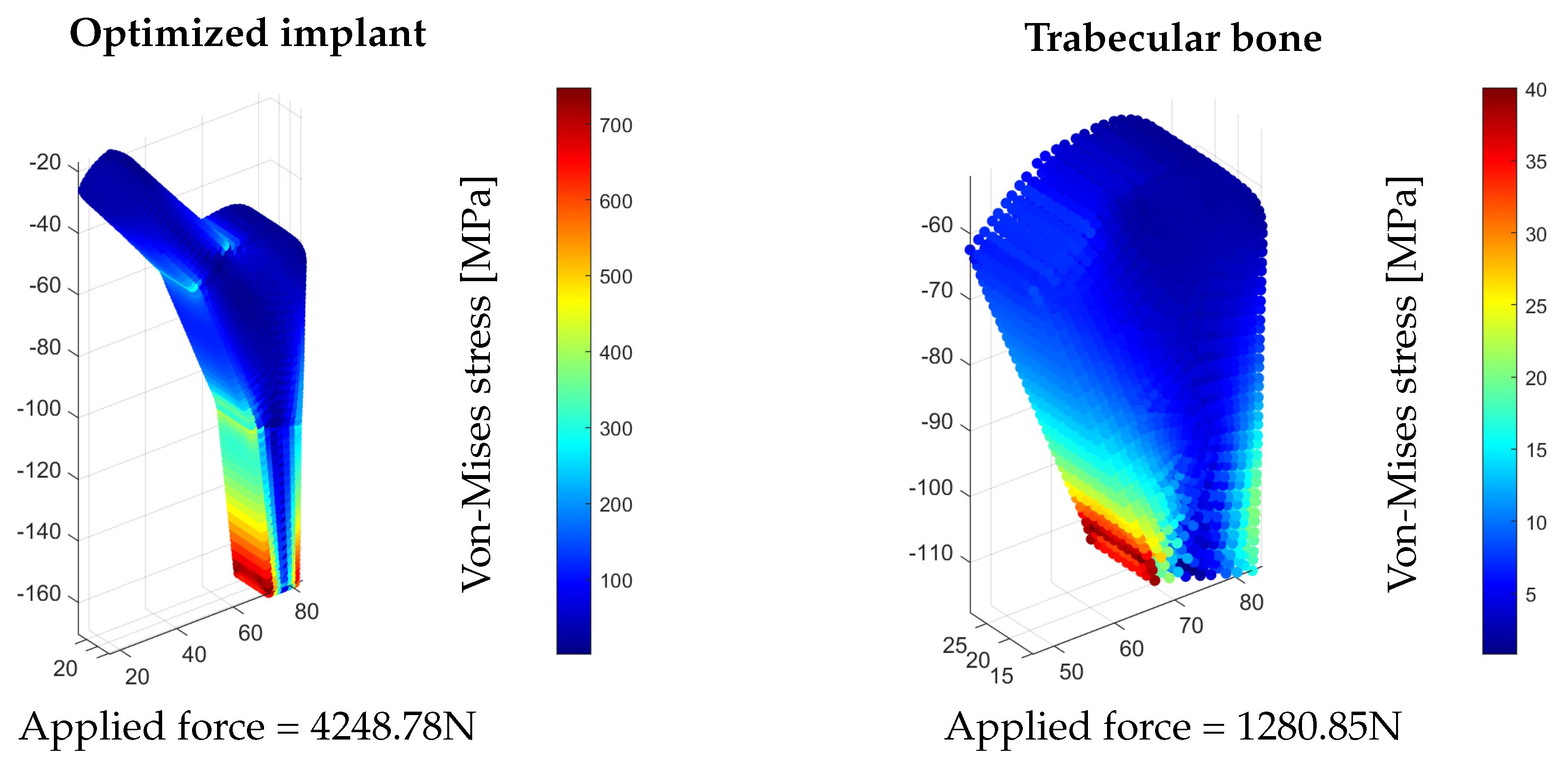
5.3. Optimized Implant
6. Conclusions
Author Contributions
Funding
Institutional Review Board Statement
Informed Consent Statement
Data Availability Statement
Conflicts of Interest
References
- Wolff, J. The Law of Bone Remodelling; Springer Science & Business Media: Berlin/Heidelberg, Germany, 2012. [Google Scholar]
- Santos, J.; Pires, T.; Gouveia, B.P.; Castro, A.P.; Fernandes, P.R. On the permeability of TPMS scaffolds. J. Mech. Behav. Biomed. Mater. 2020, 110, 103932. [Google Scholar] [CrossRef] [PubMed]
- Bobbert, F.S.; Lietaert, K.; Eftekhari, A.A.; Pouran, B.; Ahmadi, S.M.; Weinans, H.; Zadpoor, A.A. Additively manufactured metallic porous biomaterials based on minimal surfaces: A unique combination of topological, mechanical, and mass transport properties. Acta Biomater. 2017, 53, 572–584. [Google Scholar] [CrossRef] [PubMed]
- Ma, S.; Tang, Q.; Feng, Q.; Song, J.; Han, X.; Guo, F. Mechanical behaviours and mass transport properties of bone-mimicking scaffolds consisted of gyroid structures manufactured using selective laser melting. J. Mech. Behav. Biomed. Mater. 2019, 93, 158–169. [Google Scholar] [CrossRef] [PubMed]
- Al-Ketan, O.; Rowshan, R.; Abu Al-Rub, R.K. Topology-mechanical property relationship of 3D printed strut, skeletal, and sheet based periodic metallic cellular materials. Addit. Manuf. 2018, 19, 167–183. [Google Scholar] [CrossRef]
- Zhang, X.Y.; Fang, G.; Leeflang, S.; Zadpoor, A.A.; Zhou, J. Topological design, permeability and mechanical behavior of additively manufactured functionally graded porous metallic biomaterials. Acta Biomater. 2019, 84, 437–452. [Google Scholar] [CrossRef]
- Yang, L.; Yan, C.; Fan, H.; Li, Z.; Cai, C.; Chen, P.; Shi, Y.; Yang, S. Investigation on the orientation dependence of elastic response in Gyroid cellular structures. J. Mech. Behav. Biomed. Mater. 2019, 90, 73–85. [Google Scholar] [CrossRef]
- Gurra, E.; Iasiello, M.; Naso, V.; Chiu, W.K.S. Numerical prediction and correlations of effective thermal conductivity in a drilled-hollow-sphere architected foam. J. Therm. Sci. Eng. Appl. 2022, 15, 041002. [Google Scholar] [CrossRef]
- Wang, F.; Jiang, H.; Chen, Y.; Li, X. Predicting thermal and mechanical performance of stochastic and architected foams. Int. J. Heat Mass Transf. 2021, 171, 121139. [Google Scholar] [CrossRef]
- Vijayavenkataraman, S.; Kuan, L.Y.; Lu, W.F. 3D-printed ceramic triply periodic minimal surface structures for design of functionally graded bone implants. Mater. Des. 2020, 191, 108602. [Google Scholar] [CrossRef]
- Ghassemi, T.; Shahroodi, A.; Ebrahimzadeh, M.H.; Mousavian, A.; Movaffagh, J.; Moradi, A. Current concepts in scaffolding for bone tissue engineering. Arch. Bone Jt. Surg. 2018, 6, 90–99. [Google Scholar] [CrossRef] [PubMed]
- Wang, X.; Xu, S.; Zhou, S.; Xu, W.; Leary, M.; Choong, P.; Qian, M.; Brandt, M.; Xie, Y.M. Topological design and additive manufacturing of porous metals for bone scaffolds and orthopaedic implants: A review. Biomaterials 2016, 83, 127–141. [Google Scholar] [CrossRef] [PubMed]
- Ma, S.; Song, K.; Lan, J.; Ma, L. Biological and mechanical property analysis for designed heterogeneous porous scaffolds based on the refined TPMS. J. Mech. Behav. Biomed. Mater. 2020, 107, 103727. [Google Scholar] [CrossRef] [PubMed]
- Karageorgiou, V.; Kaplan, D. Porosity of 3D biomaterial scaffolds and osteogenesis. Biomaterials 2005, 26, 5474–5491. [Google Scholar] [CrossRef] [PubMed]
- Braem, A.; Chaudhari, A.; Vivan Cardoso, M.; Schrooten, J.; Duyck, J.; Vleugels, J. Peri- and intra-implant bone response to microporous Ti coatings with surface modification. Acta Biomater. 2014, 10, 986–995. [Google Scholar] [CrossRef] [PubMed]
- Itl, A.I.; Ylnen, H.O.; Ekholm, C.; Karlsson, K.H.; Aro, H.T. Pore diameter of more than 100 μm is not requisite for bone ingrowth in rabbits. J. Biomed. Mater. Res. 2001, 58, 679–683. [Google Scholar] [CrossRef]
- Taniguchi, N.; Fujibayashi, S.; Takemoto, M.; Sasaki, K.; Otsuki, B.; Nakamura, T.; Matsushita, T.; Kokubo, T.; Matsuda, S. Effect of pore size on bone ingrowth into porous titanium implants fabricated by additive manufacturing: An in vivo experiment. Mater. Sci. Eng. C 2016, 59, 690–701. [Google Scholar] [CrossRef]
- Zhang, L.; Feih, S.; Daynes, S.; Chang, S.; Wang, M.Y.; Wei, J.; Lu, W.F. Energy absorption characteristics of metallic triply periodic minimal surface sheet structures under compressive loading. Addit. Manuf. 2018, 23, 505–515. [Google Scholar] [CrossRef]
- Harrysson, O.L.; Cansizoglu, O.; Marcellin-Little, D.J.; Cormier, D.R.; West, H.A. Direct metal fabrication of titanium implants with tailored materials and mechanical properties using electron beam melting technology. Mater. Sci. Eng. C 2008, 28, 366–373. [Google Scholar] [CrossRef]
- Brian, K.; Jiang, C.; Stanford, M. An investigation into the flexural characteristics of functionally graded cobalt chrome femoral stems manufactured using selective laser melting. J. Mater. Des. 2014, 60, 177–183. [Google Scholar] [CrossRef]
- Alkhatib, S.E.; Tarlochan, F. Finite element study of functionally graded porous femoral stems incorporating body-centered cubic structure. Artif. Organs 2019, 47, E152–E164. [Google Scholar] [CrossRef]
- Munteanu, S.; Munteanu, D.; Gheorghiu, B.; Bedo, T.; Gabor, C. Additively manufactured femoral stem topology optimization: Case study. Mater. Today Proc. 2019, 19, 1019–1025. [Google Scholar] [CrossRef]
- Orellana, J.; Palacios, T.; Calle, F.; Pastor, J.Y. Bio-inspired redesign of a hip prosthesis stem for improving geometrical optimization time. Procedia Manuf. 2019, 41, 121–128. [Google Scholar] [CrossRef]
- Pais, A.I.; Alves, J.L.; Belinha, J. A bio-inspired remodelling algorithm combined with a natural neighbour meshless method to obtain optimized functionally graded materials. Eng. Anal. Bound. Elem. 2022, 135, 145–155. [Google Scholar] [CrossRef]
- Pais, A.I.; Alves, J.L.; Belinha, J. Using a radial point interpolation meshless method and the finite element method for application of a bio-inspired remodelling algorithm in the design of optimized bone scaffold. J. Braz. Soc. Mech. Sci. Eng. 2021, 43, 557. [Google Scholar] [CrossRef]
- Silva, C.M.M.d.; Pais, A.; Caldas, G.; Gouveia, B.P.; Alves, J.L.; Belinha, J. Study on 3D printing of gyroid based structures for superior structural behaviour. Prog. Addit. Manuf. 2021, 6, 689–703. [Google Scholar] [CrossRef]
- Pais, A.; Lino, J.; Jorge, A. Design of functionally graded gyroid foams using optimization A simple approach on prototyping from simulation to manufacturing. Int. J. Adv. Manuf. Technol. 2021, 114, 725–739. [Google Scholar] [CrossRef]
- Li, S.; Sitnikova, E. Representative Volume Elements and Unit Cells; Elsevier: Amsterdam, The Netherlands, 2020. [Google Scholar]
- Tian, W.; Qi, L.; Chao, X.; Liang, J.; Fu, M. Periodic boundary condition and its numerical implementation algorithm for the evaluation of effective mechanical properties of the composites with complicated micro-structures. Compos. Part B Eng. 2019, 162, 1–10. [Google Scholar] [CrossRef]
- Alwattar, T.A.; Mian, A. Development of an elastic material model for bcc lattice cell structures using finite element analysis and neural networks approaches. J. Compos. Sci. 2019, 3, 33. [Google Scholar] [CrossRef]
- Bonatti, C.; Mohr, D. Smooth-shell metamaterials of cubic symmetry: Anisotropic elasticity, yield strength and specific energy absorption. Acta Mater. 2019, 164, 301–321. [Google Scholar] [CrossRef]
- Denisiewicz, A.; Kuczma, M.; Kula, K.; Socha, T. Influence of boundary conditions on numerical homogenization of high performance concrete. Materials 2021, 14, 1009. [Google Scholar] [CrossRef] [PubMed]
- Li, D.; Liao, W.; Dai, N.; Xie, Y.M. Comparison of mechanical properties and energy absorption of sheet-based and strut-based gyroid cellular structures with graded densities. Materials 2019, 12, 2183. [Google Scholar] [CrossRef] [PubMed]
- Hinton, E. Finite elements in plasticity: Theory and practice. Appl. Ocean. Res. 1981, 3, 149. [Google Scholar] [CrossRef]
- Gibson, L.J.; Ashby, M.F. Cellular Solids: Structure and Properties; Cambridge University Press: Cambridge, UK, 1999. [Google Scholar]
- Maconachie, T.; Leary, M.; Lozanovski, B.; Zhang, X.; Qian, M.; Faruque, O.; Brandt, M. SLM lattice structures: Properties, performance, applications and challenges. Mater. Des. 2019, 183, 108137. [Google Scholar] [CrossRef]
- Li, D.; Liao, W.; Dai, N.; Dong, G.; Tang, Y.; Xie, Y.M. Optimal design and modeling of gyroid-based functionally graded cellular structures for additive manufacturing. CAD Comput. Aided Des. 2018, 104, 87–99. [Google Scholar] [CrossRef]
- Harrigan, T.P.; Hamilton, J.J. Bone remodeling and structural optimization. J. Biomech. 1994, 27, 323–328. [Google Scholar] [CrossRef]
- Belinha, J. Meshless Methods in Biomechanics: Bone Tissue Remodelling Analysis; Lecture Notes in Computational Vision and Biomechanics; Springer International Publishing: New York, NY, USA, 2014. [Google Scholar]
- Liu, B.; Wang, H.; Zhang, N.; Zhang, M.; Cheng, C.K. Femoral Stems with Porous Lattice Structures: A Review. Front. Bioeng. Biotechnol. 2021, 9, 1136. [Google Scholar] [CrossRef]
- Abueidda, D.W.; Elhebeary, M.; Shiang, C.S.A.; Pang, S.; Abu Al-Rub, R.K.; Jasiuk, I.M. Mechanical properties of 3D printed polymeric Gyroid cellular structures: Experimental and finite element study. Mater. Des. 2019, 165, 107597. [Google Scholar] [CrossRef]
- Kelly, C.N.; Francovich, J.; Julmi, S.; Safranski, D.; Guldberg, R.E.; Maier, H.J.; Gall, K. Fatigue behavior of As-built selective laser melted titanium scaffolds with sheet-based gyroid microarchitecture for bone tissue engineering. Acta Biomater. 2019, 94, 610–626. [Google Scholar] [CrossRef]
- Yu, G.; Li, Z.; Li, S.; Zhang, Q.; Hua, Y.; Liu, H.; Zhao, X.; Dhaidhai, D.T.; Li, W.; Wang, X. The select of internal architecture for porous Ti alloy scaffold: A compromise between mechanical properties and permeability. Mater. Des. 2020, 192, 108754. [Google Scholar] [CrossRef]
- Viet, N.V.; Karathanasopoulos, N.; Zaki, W. Mechanical attributes and wave propagation characteristics of TPMS lattice structures. Mech. Mater. 2022, 172, 104363. [Google Scholar] [CrossRef]
- Zhao, M.; Zhang, D.Z.; Liu, F.; Li, Z.; Ma, Z.; Ren, Z. Mechanical and energy absorption characteristics of additively manufactured functionally graded sheet lattice structures with minimal surfaces. Int. J. Mech. Sci. 2020, 167, 105262. [Google Scholar] [CrossRef]
- Al-Ketan, O.; Abu Al-Rub, R.K.; Rowshan, R. The effect of architecture on the mechanical properties of cellular structures based on the IWP minimal surface. J. Mater. Res. 2018, 33, 343–359. [Google Scholar] [CrossRef]
- Barber, H.; Kelly, C.N.; Nelson, K.; Gall, K. Compressive anisotropy of sheet and strut based porous Ti–6Al–4V scaffolds. J. Mech. Behav. Biomed. Mater. 2021, 115, 104243. [Google Scholar] [CrossRef] [PubMed]
- Ma, S.; Tang, Q.; Han, X.; Feng, Q.; Song, J.; Setchi, R.; Liu, Y.; Liu, Y.; Goulas, A.; Engstrøm, D.S.; et al. Manufacturability, Mechanical Properties, Mass-Transport Properties and Biocompatibility of Triply Periodic Minimal Surface (TPMS) Porous Scaffolds Fabricated by Selective Laser Melting. Mater. Des. 2020, 195, 109034. [Google Scholar] [CrossRef]
- Ashby, M.F.; Evans, T.; Fleck, N.A.; Hutchinson, J.W.; Wadley, H.N.G.; Gibson, L.J. Metal Foams: A Design Guide; Elsevier: Amsterdam, The Netherlands, 2000. [Google Scholar]


| SD | BD | |
|---|---|---|
| Homogenized Young’s modulus | 1 | 2 |
| Homogenized yield stress | 1 | 1.5 |
| Model | t/L |
|---|---|
| low density | 0.05 |
| medium density | 0.15 |
| high density | 0.25 |
| E* | * | C11 | C12 | C44 = G* | ||||
| primitive 1 cell | low dens | H | 61.83179 | 0.405701 | 138.6081 | 94.62162 | 48.49176 | 2.204851 |
| P | 61.75457 | 0.405275 | 137.9524 | 94.0076 | 63.79892 | 2.903592 | ||
| med dens | H | 327.7807 | 0.350119 | 526.3416 | 283.5624 | 198.3359 | 1.633879 | |
| P | 326.2036 | 0.349605 | 522.6321 | 280.929 | 222.1894 | 1.838532 | ||
| high dens | H | 818.1541 | 0.30575 | 1119.694 | 493.1158 | 396.8583 | 1.266748 | |
| P | 812.4441 | 0.305092 | 1109.737 | 487.2183 | 423.5954 | 1.360908 | ||
| E* | * | C11 | C12 | C44 = G* | ||||
| gyroid 1 cell | low dens | H | 113.7596 | 0.300448 | 153.3305 | 65.85327 | 39.45371 | 0.902034 |
| P | 155.2857 | 0.326205 | 226.9771 | 109.8868 | 65.58988 | 1.12033 | ||
| med dens | H | 560.7722 | 0.278805 | 714.874 | 276.3613 | 232.5266 | 1.060524 | |
| P | 608.784 | 0.295178 | 808.7353 | 338.6964 | 275.3023 | 1.171402 | ||
| high dens | H | 1243.97 | 0.270049 | 1554.597 | 575.1302 | 519.8329 | 1.061461 | |
| P | 1314.799 | 0.277671 | 1671.664 | 642.6045 | 572.3806 | 1.112434 | ||
| E* | * | C11 | C12 | C44 = G* | ||||
| gyroid 2 cells | low dens | H | 127.534 | 0.308422 | 175.9314 | 78.45974 | 47.83487 | 0.98151 |
| med dens | H | 578.4656 | 0.283865 | 746.4448 | 295.8789 | 252.1427 | 1.11923 | |
| high dens | H | 1292.918 | 0.270515 | 1617.423 | 599.7905 | 555.19810 | 1.09116 | |
| E* | * | C11 | C12 | C44 = G* | ||||
| gyroid 3 cells | low dens | H | 142.8026 | 0.312171 | 199.2662 | 90.43695 | 57.86529 | 1.063414 |
| med. dens | H | 622.4885 | 0.285833 | 807.1683 | 323.0553 | 274.9201 | 1.135768 |
| Low Density | |||||||||
|---|---|---|---|---|---|---|---|---|---|
| 1 × 1 × 1 | 2 × 2 × 2 | 3 × 3 × 3 | |||||||
| apparent | 0.729344 | 2.058199 | 3.253642 | 0.801418 | 2.291044 | 3.656217 | 0.836503 | 2.401517 | 3.855031 |
| apparent ratio | 0.072934 | 0.068607 | 0.065073 | 0.080142 | 0.076368 | 0.073124 | 0.08365 | 0.080051 | 0.077101 |
| mean ratio | 0.068871 | 0.076545 | 0.080267 | ||||||
| Medium Density | |||||||||
|---|---|---|---|---|---|---|---|---|---|
| 1 × 1 × 1 | 2 × 2 × 2 | 3 × 3 × 3 | |||||||
| apparent | 2.213404 | 7.271915 | 12.18746 | 3.059191 | 8.480854 | 13.66536 | 3.481273 | 9.110942 | 16.54715 |
| apparent ratio | 0.22134 | 0.242397 | 0.243749 | 0.305919 | 0.282695 | 0.273307 | 0.348127 | 0.303698 | 0.330943 |
| mean ratio | 0.235829 | 0.287307 | 0.327589 | ||||||
| High Density | |||||||||
|---|---|---|---|---|---|---|---|---|---|
| 1 × 1 × 1 | 2 × 2 × 2 | 3 × 3 × 3 | |||||||
| apparent | 5.6391 | 15.43433 | 25.32575 | 6.380779 | 17.95709 | 27.64402 | - | - | - |
| apparent ratio | 0.56391 | 0.514478 | 0.506515 | 0.638078 | 0.59857 | 0.55288 | - | - | - |
| mean ratio | 0.528301 | 0.596509 | |||||||
| Low Density | Medium Density | High Density | |||||||
|---|---|---|---|---|---|---|---|---|---|
| 2 × 2 × 2 | 2 × 2 × 2 | 1 × 1 × 1 | |||||||
| apparent | 0.7032 | 1.9971 | 3.1698 | 2.5376 | 7.887468 | 12.98112 | 4.718293 | 13.00106 | 19.45738 |
| apparent ratio | 0.07032 | 0.06657 | 0.063396 | 0.25376 | 0.262916 | 0.259622 | 0.471829 | 0.433369 | 0.389148 |
| mean ratio | 0.066762 | 0.258766 | 0.431449 | ||||||
| Gyroid | Primitive | Gyroid | Primitive | ||
|---|---|---|---|---|---|
| a | 0.1018 | 0.1766 | b | 0.5545 | 0.0000 |
| a | 0.4388 | 0.4879 | b | 0.1250 | 0.1259 |
| a | 0.2405 | 0.1157 | b | 0.4666 | 0.6655 |
| a | 0.0000 | 0.0000 | b | 0.0000 | 0.0000 |
| Relative Young’s Modulus | Relative Yield Stress | |
|---|---|---|
| Gyroid | 23.973% | 26.4787% |
| Primitive | 63.874% | 37.1244% |
| Young’s Modulus [MPa] | Yield Stress [MPa] | Poisson Ratio | |
|---|---|---|---|
| Femoral trabecular bone | 5850 | 40 | 0.3 |
| Ti-6Al-4V | 110,000 | 850 | 0.3 |
Disclaimer/Publisher’s Note: The statements, opinions and data contained in all publications are solely those of the individual author(s) and contributor(s) and not of MDPI and/or the editor(s). MDPI and/or the editor(s) disclaim responsibility for any injury to people or property resulting from any ideas, methods, instructions or products referred to in the content. |
© 2023 by the authors. Licensee MDPI, Basel, Switzerland. This article is an open access article distributed under the terms and conditions of the Creative Commons Attribution (CC BY) license (https://creativecommons.org/licenses/by/4.0/).
Share and Cite
Pais, A.; Alves, J.L.; Jorge, R.N.; Belinha, J. Multiscale Homogenization Techniques for TPMS Foam Material for Biomedical Structural Applications. Bioengineering 2023, 10, 515. https://doi.org/10.3390/bioengineering10050515
Pais A, Alves JL, Jorge RN, Belinha J. Multiscale Homogenization Techniques for TPMS Foam Material for Biomedical Structural Applications. Bioengineering. 2023; 10(5):515. https://doi.org/10.3390/bioengineering10050515
Chicago/Turabian StylePais, Ana, Jorge Lino Alves, Renato Natal Jorge, and Jorge Belinha. 2023. "Multiscale Homogenization Techniques for TPMS Foam Material for Biomedical Structural Applications" Bioengineering 10, no. 5: 515. https://doi.org/10.3390/bioengineering10050515
APA StylePais, A., Alves, J. L., Jorge, R. N., & Belinha, J. (2023). Multiscale Homogenization Techniques for TPMS Foam Material for Biomedical Structural Applications. Bioengineering, 10(5), 515. https://doi.org/10.3390/bioengineering10050515