
Fet-Net Algorithm for Automatic Detection of Fetal Orientation in Fetal MRI

 ,
,
Abstract
1. Introduction
2. Materials and Methods
2.1. Dataset
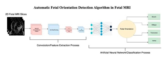
2.2. Architecture
2.3. Experiment
2.3.1. Experimentation Set-Up
2.3.2. Five-Fold Cross-Validation Experiment
2.3.3. Performance Metrics
2.3.4. Validation Experiment
2.3.5. Ablation Study
2.3.6. Signal-to-Noise Ratio Test
3. Results
3.1. Fet-Net Results
3.2. Comparison of Architectures
3.3. Validation Experiment of Fet-Net
3.4. Ablation Study
3.5. Testing on Noisy Images
4. Discussion
5. Conclusions
Author Contributions
Funding
Institutional Review Board Statement
Informed Consent Statement
Data Availability Statement
Conflicts of Interest
Abbreviations
| 2D | Two-Dimensional |
| 3D | Three-Dimensional |
| CNN | Convolutional Neural Network |
| MRI | Magnetic Resonance Imaging |
| SNR | Signal-to-Noise Ratio |
| US | Ultrasound |
References
- Australian Government Department of Health and Aged Care. Fetal Presentation. Australian Government Department of Health and Aged Care, 21 June 2018. Available online: https://www.health.gov.au/resources/pregnancy-care-guidelines/part-j-clinical-assessments-in-late-pregnancy/fetal-presentation (accessed on 6 December 2022).
- AIUM–ACR–ACOG–SMFM–SRU Practice Parameter for the Performance of Standard Diagnostic Obstetric Ultrasound Examinations. J. Ultrasound Med. 2018, 37, E13–E24. [CrossRef] [PubMed]
- Hourihane, M.J. Etiology and Management of Oblique Lie. Obstet. Gynecol. 1968, 32, 512–519. [Google Scholar] [PubMed]
- Hankins, G.D.V.; Hammond, T.L.; Snyder, R.R.; Gilstrap, L.C. Transverse Lie. Am. J. Perinatol. 1990, 7, 66–70. [Google Scholar] [CrossRef]
- Hannah, M.E.; Hannah, W.J.; Hewson, S.A.; Hodnett, E.D.; Saigal, S.; Willan, A.R. Planned caesarean section versus planned vaginal birth for breech presentation at term: A randomised multicentre trial. Lancet 2000, 356, 1375–1383. [Google Scholar] [CrossRef]
- Lyons, J.; Pressey, T.; Bartholomew, S.; Liu, S.; Liston, R.M.; Joseph, K.S.; Canadian Perinatal Surveillance System (Public Health Agency of Canada). Delivery of Breech Presentation at Term Gestation in Canada, 2003–2011. Obstet. Gynecol. 2015, 125, 1153–1161. [Google Scholar] [CrossRef] [PubMed]
- Herbst, A. Term breech delivery in Sweden: Mortality relative to fetal presentation and planned mode of delivery. Acta Obstet. Gynecol. Scand. 2005, 84, 593–601. [Google Scholar] [CrossRef]
- Patey, S.J.; Corcoran, J.P. Physics of ultrasound. Anaesth. Intensive Care Med. 2021, 22, 58–63. [Google Scholar] [CrossRef]
- Saleem, S.N. Fetal MRI: An approach to practice: A review. J. Adv. Res. 2014, 5, 507–523. [Google Scholar] [CrossRef]
- Gonçalves, L.F.; Lee, W.; Mody, S.; Shetty, A.; Sangi-Haghpeykar, H.; Romero, R. Diagnostic accuracy of ultrasonography and magnetic resonance imaging for the detection of fetal anomalies: A blinded case–control study. Ultrasound Obs. Gynecol 2016, 48, 185–192. [Google Scholar] [CrossRef]
- Levine, D. Ultrasound versus Magnetic Resonance Imaging in Fetal Evaluation. Top. Magn. Reson. Imaging 2001, 12, 25–38. [Google Scholar] [CrossRef]
- Eidelson, S.G. Save Your Aching Back and Neck: A Patient’s Guide; SYA Press and Research: Quebec, QC, Canada, 2002. [Google Scholar]
- Garel, C.; Brisse, H.; Sebag, G.; Elmaleh, M.; Oury, J.-F.; Hassan, M. Magnetic resonance imaging of the fetus. Pediatr. Radiol. 1998, 28, 201–211. [Google Scholar] [CrossRef]
- Attallah, O.; Sharkas, M.A.; Gadelkarim, H. Fetal Brain Abnormality Classification from MRI Images of Different Gestational Age. Brain Sci. 2019, 9, 231. [Google Scholar] [CrossRef] [PubMed]
- Ghadimi, M.; Sapra, A. Magnetic Resonance Imaging Contraindications. In StatPearls; StatPearls Publishing: Treasure Island, FL, USA, 2022. Available online: http://www.ncbi.nlm.nih.gov/books/NBK551669/ (accessed on 3 January 2023).
- Aertsen, M.; Diogo, M.C.; Dymarkowski, S.; Deprest, J.; Prayer, D. Fetal MRI for dummies: What the fetal medicine specialist should know about acquisitions and sequences. Prenat. Diagn. 2020, 40, 6–17. [Google Scholar] [CrossRef] [PubMed]
- Sohn, Y.-S.; Kim, M.-J.; Kwon, J.-Y.; Kim, Y.-H.; Park, Y.-W. The Usefulness of Fetal MRI for Prenatal Diagnosis. Yonsei Med. J. 2007, 48, 671–677. [Google Scholar] [CrossRef] [PubMed]
- Pimentel, I.; Costa, J.; Tavares, Ó. Fetal MRI vs. fetal ultrasound in the diagnosis of pathologies of the central nervous system. Eur. J. Public Health 2021, 31 (Suppl. 2), ckab120.079. [Google Scholar] [CrossRef]
- Prayer, D.; Malinger, G.; Brugger, P.C.; Cassady, C.; De Catte, L.; De Keersmaecker, B.; Fernandes, G.L.; Glanc, P.; Gonçalves, L.F.; Gruber, G.M.; et al. ISUOG Practice Guidelines: Performance of fetal magnetic resonance imaging. Ultrasound Obstet. Gynecol. 2017, 49, 671–680. [Google Scholar] [CrossRef]
- Valevičienė, N.R.; Varytė, G.; Zakarevičienė, J.; Kontrimavičiūtė, E.; Ramašauskaitė, D.; Rutkauskaitė-Valančienė, D. Use of Magnetic Resonance Imaging in Evaluating Fetal Brain and Abdomen Malformations during Pregnancy. Medicina 2019, 55, 55. [Google Scholar] [CrossRef]
- Nagaraj, U.D.; Kline-Fath, B.M. Clinical Applications of Fetal MRI in the Brain. Diagnostics 2020, 12, 764. [Google Scholar] [CrossRef]
- Jakhar, D.; Kaur, I. Artificial intelligence, machine learning and deep learning: Definitions and differences. Clin. Exp. Dermatol. 2020, 45, 131–132. [Google Scholar] [CrossRef]
- Goodfellow, I.; Bengio, Y.; Courville, A. Deep Learning; MIT Press: Cambridge, MA, USA, 2016. [Google Scholar]
- Irene, K.; Yudha P., A.; Haidi, H.; Faza, N.; Chandra, W. Fetal Head and Abdomen Measurement Using Convolutional Neural Network, Hough Transform, and Difference of Gaussian Revolved along Elliptical Path (Dogell) Algorithm. arXiv 2019, arXiv:1911.06298. Available online: http://arxiv.org/abs/1911.06298 (accessed on 3 December 2021).
- Lim, A.; Lo, J.; Wagner, M.W.; Ertl-Wagner, B.; Sussman, D. Automatic Artifact Detection Algorithm in Fetal MRI. Front. Artif. Intell. 2022, 5, 861791. [Google Scholar] [CrossRef] [PubMed]
- Lo, J.; Lim, A.; Wagner, M.W.; Ertl-Wagner, B.; Sussman, D. Fetal Organ Anomaly Classification Network for Identifying Organ Anomalies in Fetal MRI. Front. Artif. Intell. 2022, 5, 832485. [Google Scholar] [CrossRef] [PubMed]
- Kowsher, M.; Prottasha, N.J.; Tahabilder, A.; Habib, K.; Abdur-Rakib, M.; Alam, M.S. Predicting the Appropriate Mode of Childbirth using Machine Learning Algorithm. IJACSA Int. J. Adv. Comput. Sci. Appl. 2021, 12, 700–708. [Google Scholar] [CrossRef]
- Xu, J.; Zhang, M.; Turk, E.A.; Zhang, L.; Grant, E.; Ying, K.; Golland, P.; Adalsteinsson, E. Fetal Pose Estimation in Volumetric MRI using a 3D Convolution Neural Network. arXiv 2019, arXiv:1907.04500. Available online: http://arxiv.org/abs/1907.04500 (accessed on 9 December 2022).
- Presentation and Mechanisms of Labor|GLOWM. Available online: http://www.glowm.com/section-view/heading/PresentationandMechanismsofLabor/item/126 (accessed on 19 December 2022).
- Wu, Z.; Ramsundar, B.; Feinberg, E.N.; Gomes, J.; Geniesse, C.; Pappu, A.S.; Leswing, K.; Pande, V. MoleculeNet: A benchmark for molecular machine learning. Chem. Sci. 2018, 9, 513–530. [Google Scholar] [CrossRef]
- Madaan, V.; Roy, A.; Gupta, C.; Agrawal, P.; Sharma, A.; Bologa, C.; Prodan, R. XCOVNet: Chest X-ray Image Classification for COVID-19 Early Detection Using Convolutional Neural Networks. New Gener. Comput. 2021, 39, 583–597. [Google Scholar] [CrossRef]
- Haque, K.F.; Abdelgawad, A. A Deep Learning Approach to Detect COVID-19 Patients from Chest X-ray Images. AI 2020, 1, 418–435. [Google Scholar] [CrossRef]
- Lin, G.; Shen, W. Research on convolutional neural network based on improved Relu piecewise activation function. Procedia Comput. Sci. 2018, 131, 977–984. [Google Scholar] [CrossRef]
- Habibi Aghdam, H.; Jahani Heravi, E. Guide to Convolutional Neural Networks: A Practical Application to Traffic-Sign Detection and Classification; Springer International Publishing AG: Cham, Switzerland, 2017; Available online: http://ebookcentral.proquest.com/lib/ryerson/detail.action?docID=4862504 (accessed on 17 February 2022).
- Zhang, Z. Improved Adam Optimizer for Deep Neural Networks. In Proceedings of the 2018 IEEE/ACM 26th International Symposium on Quality of Service (IWQoS), Banff, AB, Canada, 4–6 June 2018; pp. 1–2. [Google Scholar] [CrossRef]
- Meyes, R.; Lu, M.; de Puiseau, C.W.; Meisen, T. Ablation Studies in Artificial Neural Networks. arXiv 2019, arXiv:1901.08644. [Google Scholar]
- Weishaupt, D.; Köchli, V.D.; Marincek, B. Factors Affecting the Signal-to-Noise Ratio. In How Does MRI Work? An Introduction to the Physics and Function of Magnetic Resonance Imaging; Weishaupt, D., Köchli, V.D., Marincek, B., Eds.; Springer: Berlin/Heidelberg, Germany, 2003; pp. 31–42. [Google Scholar] [CrossRef]


| Vertex | Breech | Oblique | Transverse | |
|---|---|---|---|---|
| Average Precision (%) | 99.35 | 99.35 | 96.12 | 95.87 |
| Average Recall (%) | 99.93 | 99.80 | 95.23 | 95.75 |
| Average F1-Score (%) | 99.64 | 99.57 | 95.67 | 95.81 |
| Architecture | Average Accuracy (%) | Average Loss | Number of Parameters |
|---|---|---|---|
| Fet-Net | 97.68 | 0.06828 | 10,556,420 |
| VGG16 | 96.72 | 0.12316 | 14,847,044 |
| VGG19 | 95.83 | 0.15412 | 20,156,740 |
| ResNet-50 | 88.37 | 0.40604 | 24,113,284 |
| ResNet-50V2 | 95.20 | 0.16328 | 24,090,372 |
| ResNet-101 | 82.12 | 0.47086 | 43,183,748 |
| ResNet-101V2 | 94.69 | 0.18866 | 43,152,132 |
| ResNet-152 | 84.12 | 0.41756 | 58,896,516 |
| ResNet-152V2 | 94.61 | 0.20502 | 58,857,220 |
| Inception-ResnetV2 | 94.20 | 0.21042 | 54,731,236 |
| InceptionV3 | 93.83 | 0.21720 | 22,328,356 |
| Xception | 96.08 | 0.13956 | 21,387,052 |
| Architecture | Accuracy (%) | Loss | Number of Parameters |
|---|---|---|---|
| Fet-Net (Average of 3 Seeds) | 82.20 | 0.4777 | 10,556,420 |
| VGG16 | 63.80 | 1.6586 | 14,847,044 |
| VGG19 | 61.82 | 1.6588 | 20,156,740 |
| ResNet-50 | 53.06 | 1.7716 | 24,113,284 |
| ResNet-50V2 | 70.58 | 1.1676 | 24,090,372 |
| ResNet-101 | 57.85 | 1.3354 | 43,183,748 |
| ResNet-101V2 | 66.12 | 1.4789 | 43,152,132 |
| ResNet-152 | 60.00 | 1.2846 | 58,896,516 |
| ResNet-152V2 | 76.86 | 1.0471 | 58,857,220 |
| Inception-ResNetV2 | 63.64 | 1.5332 | 54,731,236 |
| InceptionV3 | 59.17 | 1.7725 | 22,328,356 |
| Xception | 62.48 | 1.5365 | 21,387,052 |
| Component(s) Removed (Sequentially) | Average Accuracy (%) | Average Loss | Number of Parameters |
|---|---|---|---|
| Full Architecture | 97.68 | 0.06828 | 10,556,420 |
| Dropout in Feature Extraction Section | 96.58 | 0.1614 | 10,561,028 |
| Dropout in Feature Extraction and Classification Sections | 94.97 | 0.30464 | 10,561,028 |
| Dense Layer with 256 Neurons | 94.51 | 0.28262 | 4,237,572 |
| Second Convolutional Layer with 512 Filters | 91.70 | 0.54048 | 2,238,212 |
| First Convolutional Layer with 512 Filters | 88.38 | 0.92238 | 1,518,852 |
| Second Convolutional Layer with 256 Filters | 87.11 | 0.75504 | 3,693,572 |
| First Convolutional Layer with 256 Filters (1 filter left for functional purposes) | 78.84 | 1.11718 | 14,432 |
| Architecture | Accuracy (%) | Loss |
|---|---|---|
| Fet-Net | 74.58 | 0.7491 |
| VGG16 | 67.50 | 1.4996 |
| VGG19 | 49.58 | 2.8058 |
| ResNet-50 | 69.58 | 0.8897 |
| ResNet-50V2 | 55.83 | 2.0550 |
| ResNet-101 | 60.00 | 0.9695 |
| ResNet-101V2 | 61.25 | 2.6991 |
| ResNet-152 | 70.83 | 0.7185 |
| ResNet-152V2 | 57.50 | 2.3606 |
| Inception-Resnet-V2 | 66.67 | 1.2373 |
| InceptionV3 | 56.57 | 2.6833 |
| Xception | 62.92 | 1.9649 |
Disclaimer/Publisher’s Note: The statements, opinions and data contained in all publications are solely those of the individual author(s) and contributor(s) and not of MDPI and/or the editor(s). MDPI and/or the editor(s) disclaim responsibility for any injury to people or property resulting from any ideas, methods, instructions or products referred to in the content. |
© 2023 by the authors. Licensee MDPI, Basel, Switzerland. This article is an open access article distributed under the terms and conditions of the Creative Commons Attribution (CC BY) license (https://creativecommons.org/licenses/by/4.0/).
Share and Cite
Eisenstat, J.; Wagner, M.W.; Vidarsson, L.; Ertl-Wagner, B.; Sussman, D. Fet-Net Algorithm for Automatic Detection of Fetal Orientation in Fetal MRI. Bioengineering 2023, 10, 140. https://doi.org/10.3390/bioengineering10020140
Eisenstat J, Wagner MW, Vidarsson L, Ertl-Wagner B, Sussman D. Fet-Net Algorithm for Automatic Detection of Fetal Orientation in Fetal MRI. Bioengineering. 2023; 10(2):140. https://doi.org/10.3390/bioengineering10020140
Chicago/Turabian StyleEisenstat, Joshua, Matthias W. Wagner, Logi Vidarsson, Birgit Ertl-Wagner, and Dafna Sussman. 2023. "Fet-Net Algorithm for Automatic Detection of Fetal Orientation in Fetal MRI" Bioengineering 10, no. 2: 140. https://doi.org/10.3390/bioengineering10020140
APA StyleEisenstat, J., Wagner, M. W., Vidarsson, L., Ertl-Wagner, B., & Sussman, D. (2023). Fet-Net Algorithm for Automatic Detection of Fetal Orientation in Fetal MRI. Bioengineering, 10(2), 140. https://doi.org/10.3390/bioengineering10020140