
On the Alignment of Acoustic and Coupled Mechanic-Acoustic Eigenmodes in Phonation by Supraglottal Duct Variations

 , , , , , , and
Abstract
:1. Introduction
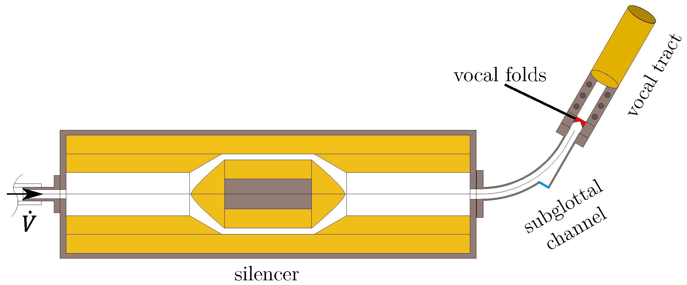
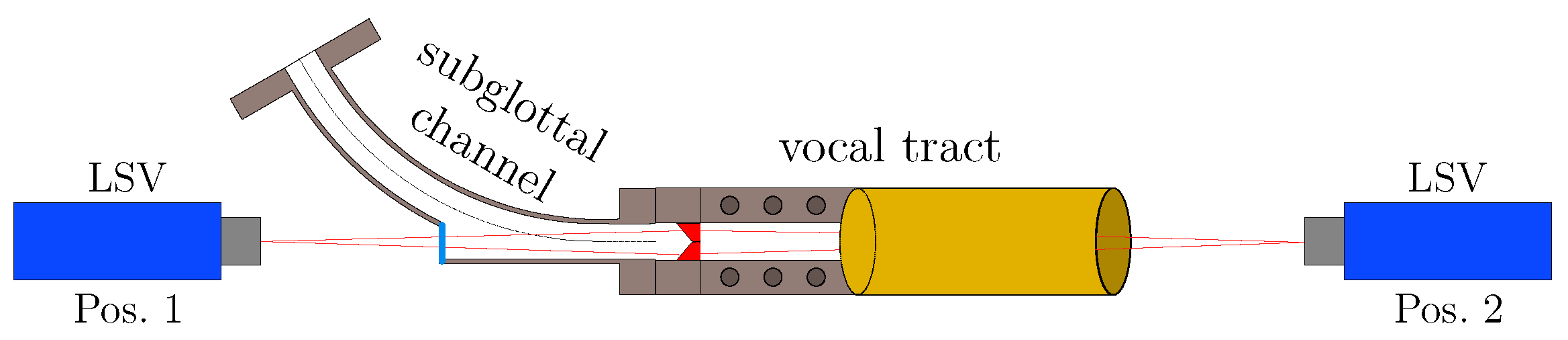
2. Experimental Study
3. Numerical Model
3.1. Governing Equations
3.1.1. Acoustic Field
3.1.2. Mechanic Field
3.1.3. Finite Element Formulation of Mechanic-Acoustic Coupling
3.2. Eigenvalue Problem
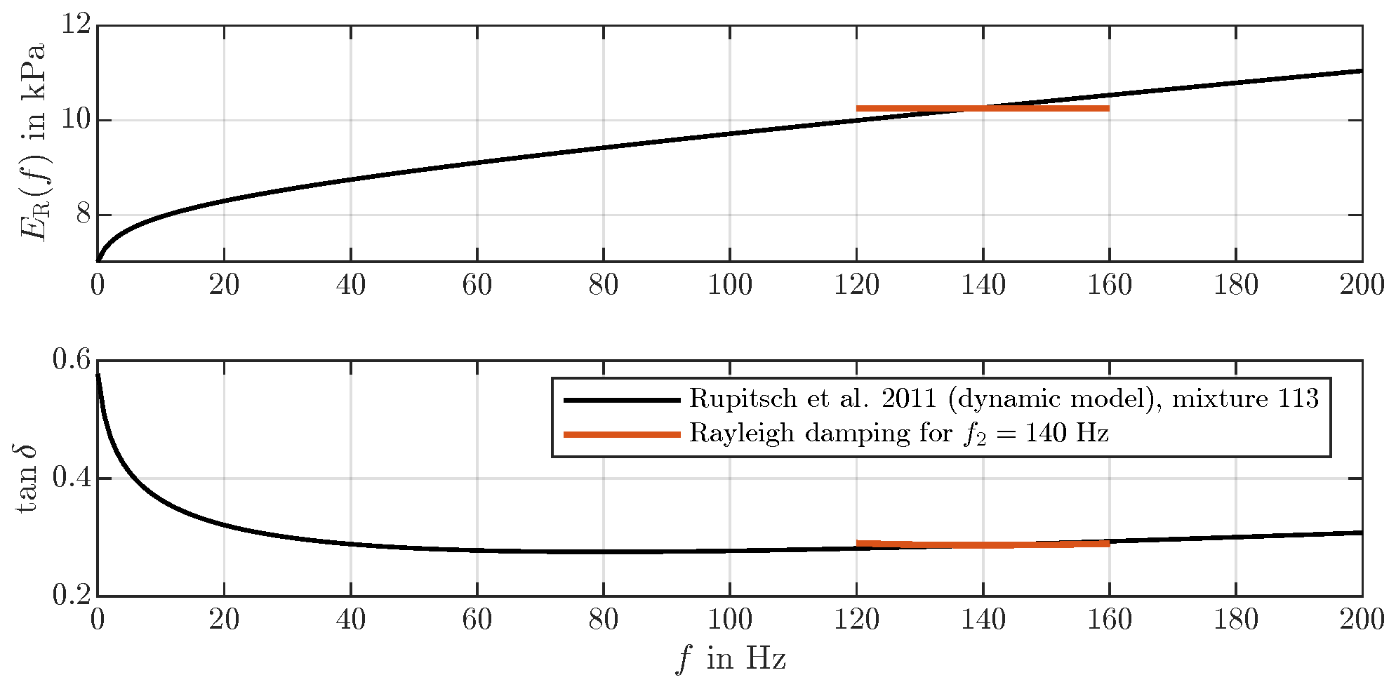
3.3. Material Damping Model
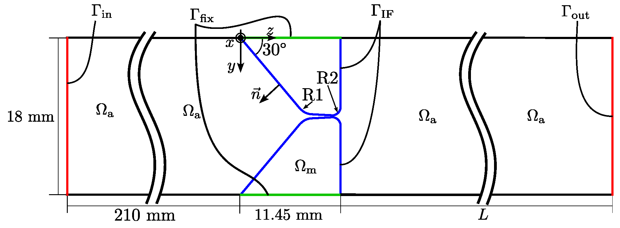
3.4. Simulation Setup
3.5. Mesh Convergence Study
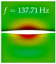
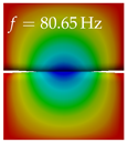
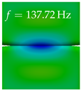
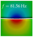
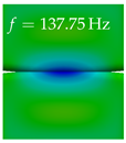
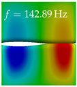
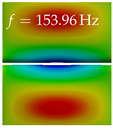
4. Results
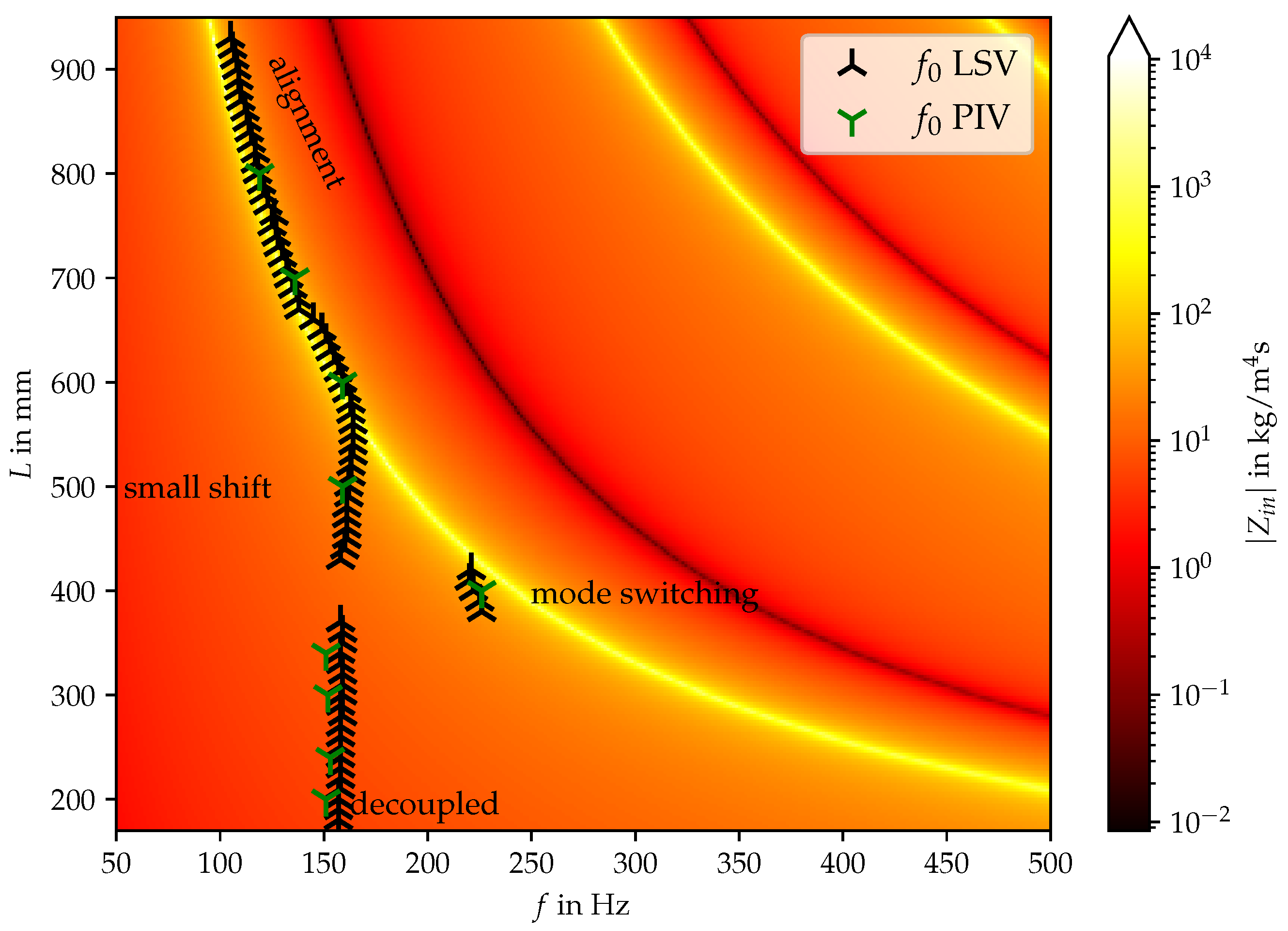
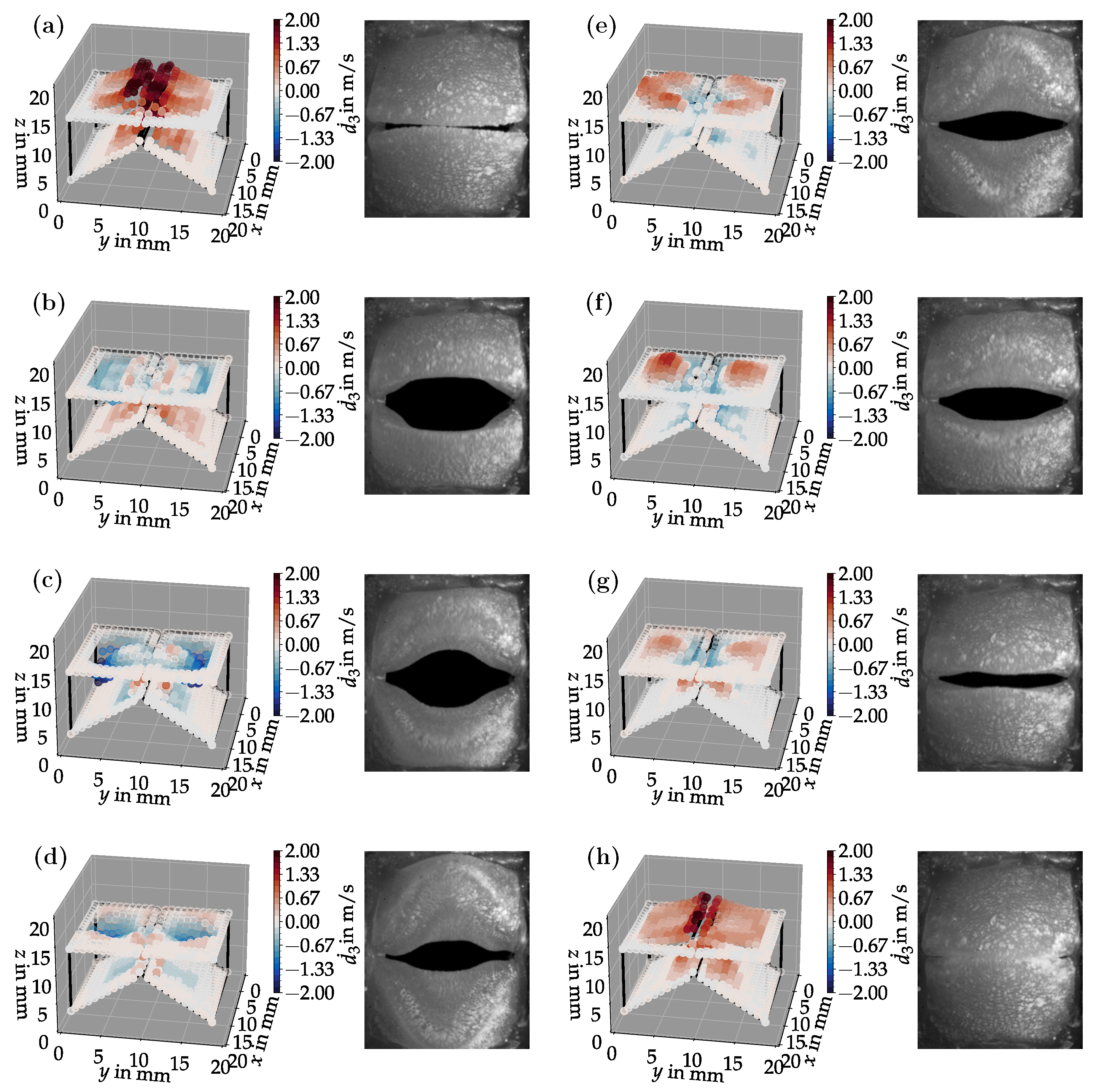
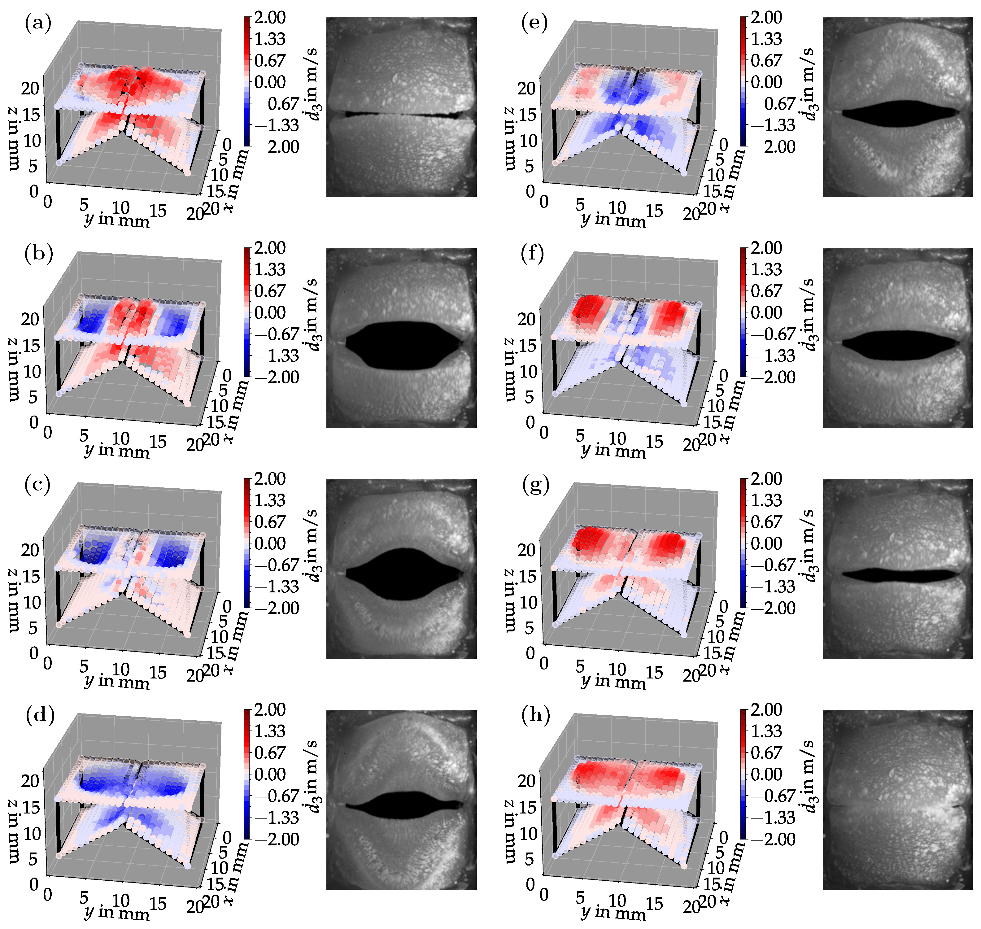
4.1. Experimental Results
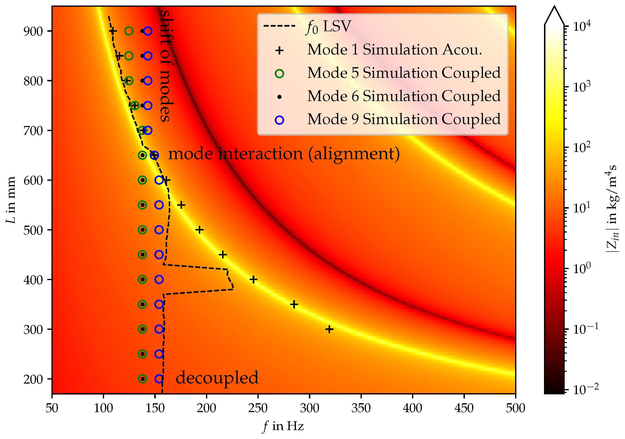
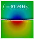
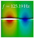
4.2. Numerical Results
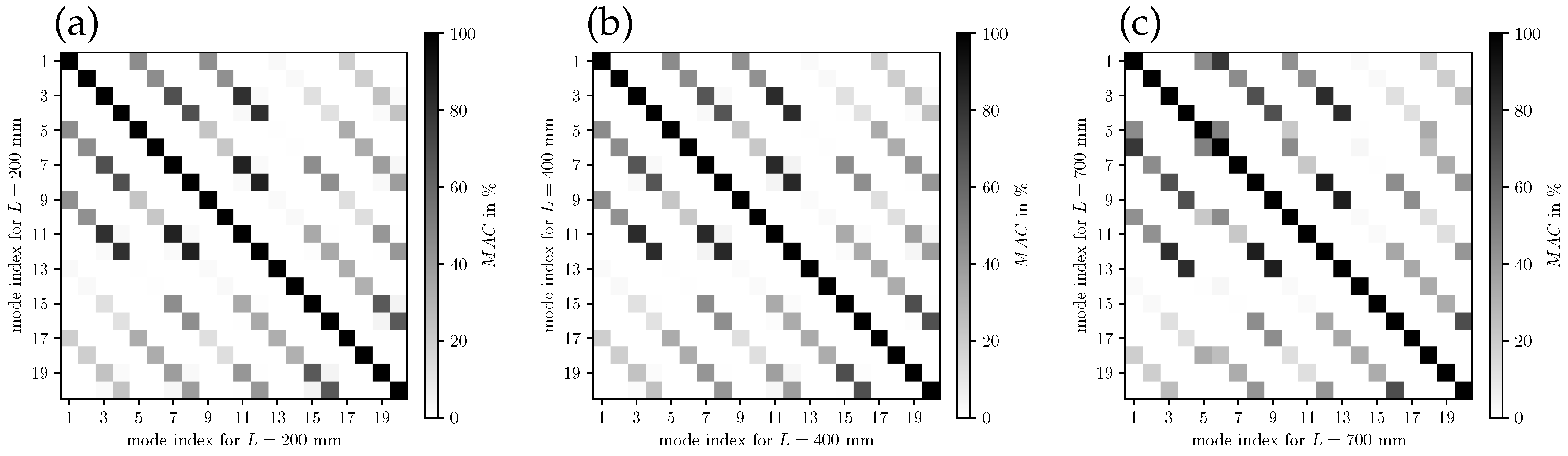
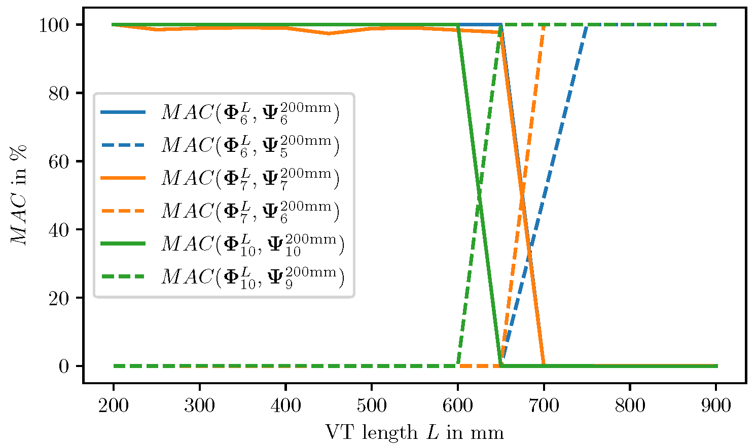
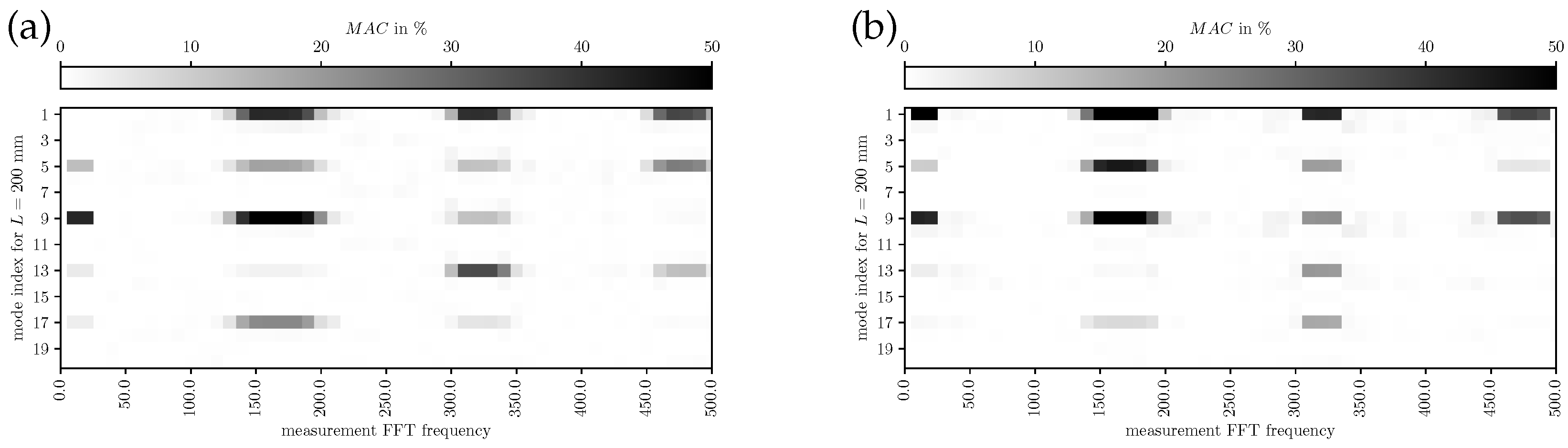
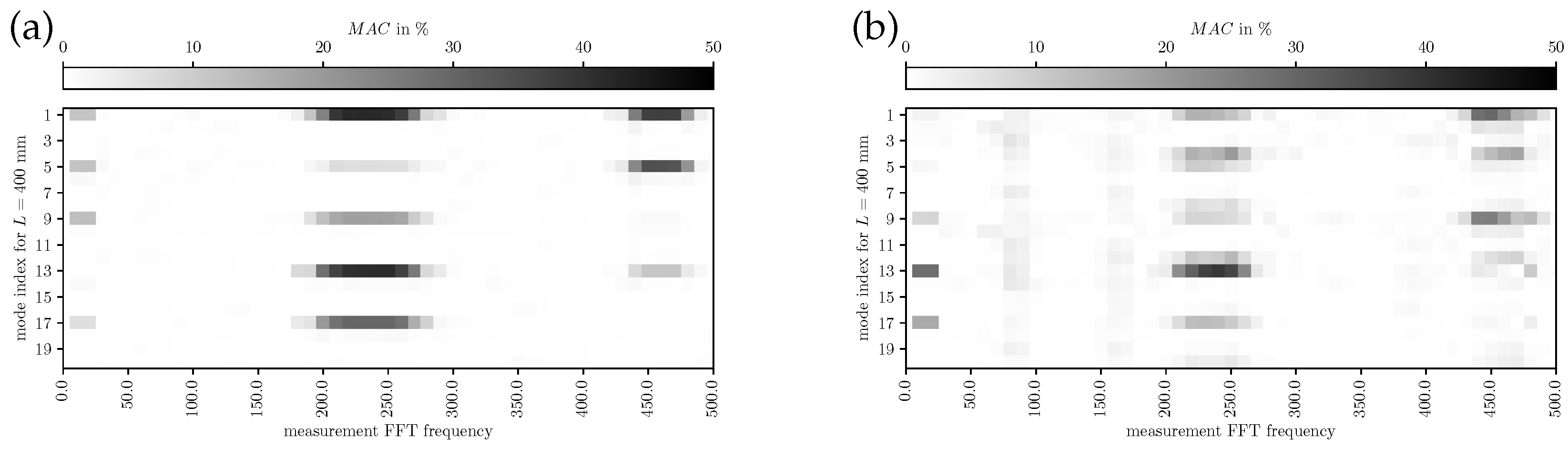
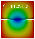
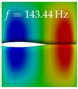
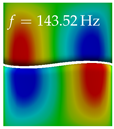
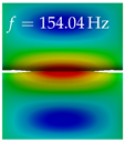
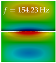
4.3. Comparison of Experimental and Numerical Results by Modal Assurance Criterion
5. Discussion
5.1. Model Limitations
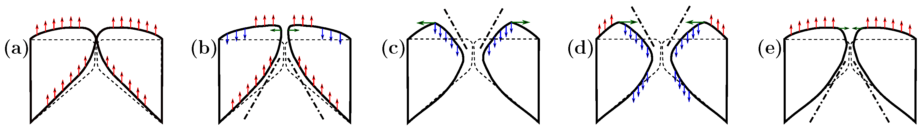
5.2. Oscillation Pattern and Relation to Other Voice Parameters
6. Conclusions
Author Contributions
Funding
Institutional Review Board Statement
Informed Consent Statement
Data Availability Statement
Acknowledgments
Conflicts of Interest
References
- Döllinger, M.; Zhang, Z.; Schoder, S.; Šidlof, P.; Tur, B.; Kniesburges, S. Overview on state-of-the-art numerical modeling of the phonation process. Acta Acust. 2023, 7, 25. [Google Scholar] [CrossRef]
- Schoder, S.; Maurerlehner, P.; Wurzinger, A.; Hauser, A.; Falk, S.; Kniesburges, S.; Döllinger, M.; Kaltenbacher, M. Aeroacoustic sound source characterization of the human voice production-perturbed convective wave equation. Appl. Sci. 2021, 11, 2614. [Google Scholar] [CrossRef]
- Maurerlehner, P.; Schoder, S.; Freidhager, C.; Wurzinger, A.; Hauser, A.; Kraxberger, F.; Falk, S.; Kniesburges, S.; Echternach, M.; Döllinger, M.; et al. Efficient numerical simulation of the human voice: simVoice—A three-dimensional simulation model based on a hybrid aeroacoustic approach. e i Elektrotech. Informationstechnik 2021, 138, 219–228. [Google Scholar] [CrossRef]
- Schoder, S.; Kraxberger, F.; Falk, S.; Wurzinger, A.; Roppert, K.; Kniesburges, S.; Döllinger, M.; Kaltenbacher, M. Error detection and filtering of incompressible flow simulations for aeroacoustic predictions of human voice. J. Acoust. Soc. Am. 2022, 152, 1425–1436. [Google Scholar] [CrossRef] [PubMed]
- Zhang, Z. Cause-effect relationship between vocal fold physiology and voice production in a three-dimensional phonation model. J. Acoust. Soc. Am. 2016, 139, 1493–1507. [Google Scholar] [CrossRef] [PubMed]
- Fant, G. Acoustic Theory of Speech Production: With Calculations Based on X-ray Studies of Russian Articulations; Number 2; Walter de Gruyter: Berlin, Germany, 1971. [Google Scholar] [CrossRef]
- Titze, I.R. Nonlinear source–filter coupling in phonation: Theory. J. Acoust. Soc. Am. 2008, 123, 2733–2749. [Google Scholar] [CrossRef]
- Sundberg, J.; Lã, F.; Granqvist, S. Fundamental frequency disturbances in female and male singers’ pitch glides through long tube with varied resistances. J. Acoust. Soc. Am. 2023, 154, 801–807. [Google Scholar] [CrossRef]
- Lucero, J.C.; Lourenço, K.G.; Hermant, N.; Van Hirtum, A.; Pelorson, X. Effect of source–tract acoustical coupling on the oscillation onset of the vocal folds. J. Acoust. Soc. Am. 2012, 132, 403–411. [Google Scholar] [CrossRef]
- Zhang, Z.; Neubauer, J.; Berry, D.A. Aerodynamically and acoustically driven modes of vibration in a physical model of the vocal folds. J. Acoust. Soc. Am. 2006, 120, 2841–2849. [Google Scholar] [CrossRef]
- Zhang, Z.; Neubauer, J.; Berry, D.A. Influence of vocal fold stiffness and acoustic loading on flow-induced vibration of a single-layer vocal fold model. J. Sound Vib. 2009, 322, 299–313. [Google Scholar] [CrossRef]
- Echternach, M.; Herbst, C.T.; Köberlein, M.; Story, B.; Döllinger, M.; Gellrich, D. Are source-filter interactions detectable in classical singing during vowel glides? J. Acoust. Soc. Am. 2021, 149, 4565–4578. [Google Scholar] [CrossRef] [PubMed]
- Migimatsu, K.; Tokuda, I.T. Experimental study on nonlinear source–filter interaction using synthetic vocal fold models. J. Acoust. Soc. Am. 2019, 146, 983–997. [Google Scholar] [CrossRef] [PubMed]
- Näger, C.; Lodermeyer, A.; Becker, S. Charakterisierung der Stimmlippenvibration an einem synthetischen Larynx-Modell mittels Laser-Scanning-Vibrometrie. In Proceedings of the DAGA 2022, Stuttgart, Germany, 21–24 March 2022; pp. 927–930. [Google Scholar]
- Näger, C.; Kniesburges, S.; Becker, S. Investigation of Acoustic Back-coupling in Human Phonation via Particle Image Velocimetry. In Proceedings of the Forum Acusticum 2023, Torino, Italy, 11–15 September 2023. [Google Scholar]
- Falk, S.; Kniesburges, S.; Schoder, S.; Jakubaß, B.; Maurerlehner, P.; Echternach, M.; Kaltenbacher, M.; Döllinger, M. 3D-FV-FE aeroacoustic larynx model for investigation of functional based voice disorders. Front. Physiol. 2021, 12, 616985. [Google Scholar] [CrossRef] [PubMed]
- Scherer, R.C.; Shinwari, D.; De Witt, K.J.; Zhang, C.; Kucinschi, B.R.; Afjeh, A.A. Intraglottal pressure profiles for a symmetric and oblique glottis with a divergence angle of 10 degrees. J. Acoust. Soc. Am. 2001, 109, 1616–1630. [Google Scholar] [CrossRef] [PubMed]
- Rupitsch, S.J.; Ilg, J.; Sutor, A.; Lerch, R.; Döllinger, M. Simulation based estimation of dynamic mechanical properties for viscoelastic materials used for vocal fold models. J. Sound Vib. 2011, 330, 4447–4459. [Google Scholar] [CrossRef]
- Durst, F.; Heim, U.; Ünsal, B.; Kullik, G. Mass flow rate control system for time-dependent laminar and turbulent flow investigations. Meas. Sci. Technol. 2003, 14, 893. [Google Scholar] [CrossRef]
- Lodermeyer, A.; Becker, S.; Döllinger, M.; Kniesburges, S. Phase-locked flow field analysis in a synthetic human larynx model. Exp. Fluids 2015, 56, 1–13. [Google Scholar] [CrossRef]
- Lodermeyer, A.; Bagheri, E.; Kniesburges, S.; Näger, C.; Probst, J.; Döllinger, M.; Becker, S. The mechanisms of harmonic sound generation during phonation: A multi-modal measurement-based approach. J. Acoust. Soc. Am. 2021, 150, 3485–3499. [Google Scholar] [CrossRef]
- ANSYS, Inc. Ansys Mechanical, Release 2022 R2; ANSYS, Inc.: Canonsburg, PA, USA, 2022. [Google Scholar]
- ANSYS, Inc. Theory Reference for the Mechanical APDL and Mechanical Applications; Kohnke, P., Ed.; Technical Report; ANSYS, Inc.: Canonsburg, PA, USA, 2009. [Google Scholar]
- Kaltenbacher, M. Numerical Simulation of Mechatronic Sensors and Actuators, 3rd ed.; Springer: Berlin/Heidelberg, Germany, 2015. [Google Scholar] [CrossRef]
- Dabbaghchian, S.; Arnela, M.; Engwall, O.; Guasch, O. Simulation of vowel-vowel utterances using a 3D biomechanical-acoustic model. Int. J. Numer. Methods Biomed. Eng. 2021, 37, e3407. [Google Scholar] [CrossRef]
- Story, B.H.; Laukkanen, A.M.; Titze, I.R. Acoustic impedance of an artificially lengthened and constricted vocal tract. J. Voice 2000, 14, 455–469. [Google Scholar] [CrossRef]
- Murray, P.R.; Thomson, S.L. Vibratory responses of synthetic, self-oscillating vocal fold models. J. Acoust. Soc. Am. 2012, 132, 3428–3438. [Google Scholar] [CrossRef] [PubMed]
- Kraxberger, F.; Museljic, E.; Kurz, E.; Toth, F.; Kaltenbacher, M.; Schoder, S. The Nonlinear Eigenfrequency Problem of Room Acoustics with Porous Edge Absorbers. In Proceedings of the Forum Acusticum 2023, European Acoustics Association, Torino, Italy, 11–15 September 2023. [Google Scholar]
- Kraxberger, F.; Kurz, E.; Weselak, W.; Kubin, G.; Kaltenbacher, M.; Schoder, S. A Validated Finite Element Model for Room Acoustic Treatments with Edge Absorbers. Acta Acust. 2023, 7, 1–19. [Google Scholar] [CrossRef]
- Sondhi, M.; Schroeter, J. A hybrid time-frequency domain articulatory speech synthesizer. IEEE Trans. Acoust. Speech Signal Process. 1987, 35, 955–967. [Google Scholar] [CrossRef]
- Näger, C.; Kniesburges, S.; Tur, B.; Schoder, S.; Becker, S. Investigation of Acoustic Back-coupling in Human Phonation on a Synthetic Larynx Model. Bioengineering 2023, 10, 1343. [Google Scholar] [CrossRef]
- Titze, I.R.; Martin, D.W. Principles of Voice Production; Acoustical Society of America: Melville, NY, USA, 1998. [Google Scholar]
- Pastor, M.; Binda, M.; Harčarik, T. Modal assurance criterion. Procedia Eng. 2012, 48, 543–548. [Google Scholar] [CrossRef]
- Herzel, H.; Berry, D.; Titze, I.R.; Saleh, M. Analysis of vocal disorders with methods from nonlinear dynamics. J. Speech Lang. Hear. Res. 1994, 37, 1008–1019. [Google Scholar] [CrossRef] [PubMed]
- Titze, I.R. How can vocal folds oscillate with a limited mucosal wave? JASA Express Lett. 2022, 2, 105201. [Google Scholar] [CrossRef] [PubMed]
- Sundström, E.; Oren, L.; de Luzan, C.F.; Gutmark, E.; Khosla, S. Fluid-Structure Interaction Analysis of Aerodynamic and Elasticity Forces During Vocal Fold Vibration. J. Voice 2022. [CrossRef]
- Titze, I.R. Theoretical analysis of maximum flow declination rate versus maximum area declination rate in phonation. J. Speech Lang. Hear. Res. 2006, 49, 439–447. [Google Scholar] [CrossRef]
- Manconi, E.; Mace, B.R.; Garziera, R. Wave Propagation in Laminated Cylinders with Internal Fluid and Residual Stress. Appl. Sci. 2023, 13, 5227. [Google Scholar] [CrossRef]


| 7.02 kPa |
| Mesh | Approx. Elem. Size (in mm) | Wavelength at f = 8.5 kHz | ||||
|---|---|---|---|---|---|---|
| Duct | VT | Duct | VT | |||
| mesh 1 | ||||||
| mesh 2 | ||||||
| mesh 3 (reference) | — | |||||
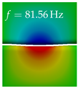
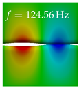
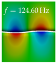
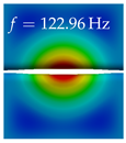
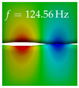
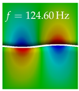
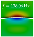
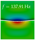
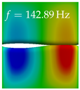
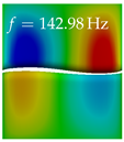
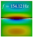
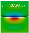
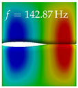
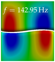
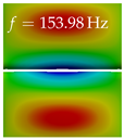
| VT Length | Mode Index 1 | Mode Index 2 | Mode Index 3 | Mode Index 4 | Mode Index 5 |
|---|---|---|---|---|---|
 |  |  |  | 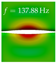 | |
 |  |  |  |  | |
 |  |  |  |  | |
 |  |  |  |  | |
| VT Length | Mode Index 6 | Mode Index 7 | Mode Index 8 | Mode Index 9 | Mode Index 10 |
 |  |  |  |  | |
 |  |  |  |  | |
 |  |  |  |  | |
 |  |  |  |  |
Disclaimer/Publisher’s Note: The statements, opinions and data contained in all publications are solely those of the individual author(s) and contributor(s) and not of MDPI and/or the editor(s). MDPI and/or the editor(s) disclaim responsibility for any injury to people or property resulting from any ideas, methods, instructions or products referred to in the content. |
© 2023 by the authors. Licensee MDPI, Basel, Switzerland. This article is an open access article distributed under the terms and conditions of the Creative Commons Attribution (CC BY) license (https://creativecommons.org/licenses/by/4.0/).
Share and Cite
Kraxberger, F.; Näger, C.; Laudato, M.; Sundström, E.; Becker, S.; Mihaescu, M.; Kniesburges, S.; Schoder, S. On the Alignment of Acoustic and Coupled Mechanic-Acoustic Eigenmodes in Phonation by Supraglottal Duct Variations. Bioengineering 2023, 10, 1369. https://doi.org/10.3390/bioengineering10121369
Kraxberger F, Näger C, Laudato M, Sundström E, Becker S, Mihaescu M, Kniesburges S, Schoder S. On the Alignment of Acoustic and Coupled Mechanic-Acoustic Eigenmodes in Phonation by Supraglottal Duct Variations. Bioengineering. 2023; 10(12):1369. https://doi.org/10.3390/bioengineering10121369
Chicago/Turabian StyleKraxberger, Florian, Christoph Näger, Marco Laudato, Elias Sundström, Stefan Becker, Mihai Mihaescu, Stefan Kniesburges, and Stefan Schoder. 2023. "On the Alignment of Acoustic and Coupled Mechanic-Acoustic Eigenmodes in Phonation by Supraglottal Duct Variations" Bioengineering 10, no. 12: 1369. https://doi.org/10.3390/bioengineering10121369
APA StyleKraxberger, F., Näger, C., Laudato, M., Sundström, E., Becker, S., Mihaescu, M., Kniesburges, S., & Schoder, S. (2023). On the Alignment of Acoustic and Coupled Mechanic-Acoustic Eigenmodes in Phonation by Supraglottal Duct Variations. Bioengineering, 10(12), 1369. https://doi.org/10.3390/bioengineering10121369