A Comparative Evaluation of Using Rain Gauge and NEXRAD Radar-Estimated Rainfall Data for Simulating Streamflow

Abstract

Ascertaining the spatiotemporal accuracy of precipitation is a challenge for hydrologists and planners for flood protection measures. The objective of this study was to compare streamflow simulations using rain gauge and radar data from a watershed in Southern Ontario, Canada, using the Hydrologic Engineering Center’s event-based distributed Hydrologic Modeling System (HEC-HMS). The model was run using the curve number (CN) and the Green and Ampt infiltration methods. The results show that the streamflow simulated with rain gauge data compared better with the observed streamflow than the streamflow simulated using radar data. However, when the Mean Field Bias (MFB) corrections were applied, the quality of the streamflow results obtained from radar rainfall data improved. The results showed no significant difference between the simulated streamflow using the SCS and the Green and Ampt infiltration approach. However, the SCS method is reasonably more appropriate for modeling the runoff at the sub-basin-scale than the Green and Ampt infiltration approach. With the SCS method, the simulated and observed runoff amount obtained using rain gauge rainfall showed an R² value of 0.88 and 0.78 for MFB-corrected radar and 0.75 for radar only. For the Green and Ampt modeling option, the R² value for the simulated and observed runoff amounts were 0.87 with rain gauge, 0.66 with radar only, and 0.68 with MFB-corrected radar rainfall inputs. The NSE values for rain gauge input ranged from 0.65 to 0.35. Overall, three values were less than 0.5 for streamflow for both the methods. For seven radar rainfall events, the NSE was greater than 0.5, with a range of very good to satisfactory. The analysis of RSR showed a very good comparison of stream flow using the SCS curve number method and Green and Ampt method using different rainfall inputs. Only one value, the 2 November 2003 event, was above 0.7 for rain gauge-based streamflow. The other RSR values were in the range of “very good”. Overall, the study showed better results for the simulated runoff with the MFB-corrected radar rainfall when compared with the simulations obtained using radar rainfall only. Therefore, MFB-corrected radar could be explored as a substitute rainfall source.

1. Introduction

In hydrology, a key factor for accurate flood estimates is to have reliable spatial and temporal measurement of rainfall. Typically, rain gauges and radars are used for the measurement and estimation of rainfall. Rain gauges are generally considered as accurate estimates of precipitation near the ground surface; however, recording the spatial variability of rainfall at the watershed scale is difficult [1,2]. The precipitation data are collected by measuring rainfall at the ground using rain gauges, satellite, and weather radar [3,4]. Rain gauges provide rainfall measurements for a particular point where the rain gauge is located. Depending on the spatial distribution of rain within the watershed, these point-measurements of rainfall can significantly affect the estimation of streamflow. On the other hand, the radar-rainfall measurement technique can provide the spatial distribution of rainfall with the watershed. The radar detects raindrops by emitting out a pulse of electromagnetic energy from the radar station and then measures the energy reflected from the rain [5]. GRCA’s study also indicated that the potential of underestimation (most common) and overestimation error exists for the rainfall measurement through radar. Hence, for the reliability of results, estimation through rain gauge and radar needs further development or corroboration. Nonetheless, reports favor radar rainfall technology since a single site can obtain coverage over a wide area with a high temporal and spatial resolution [6].

Both networks, rain gauge and radar, have some limitations in accurate measurement and estimation of rainfall at the watershed scale. These limitations include a sparse rain gauge network to cover the large watersheds and the difficulty of forecasting rainfall with a longer lead time based on rain gauge data only [7,8]. However, radar systems have the ability to observe the spatial variability of rainfall for large areas that can improve the short-term prediction of rainfall for an area. Nevertheless, the accuracy of radar measurements is not up to the mark for extreme rainfall events [9,10]. The reason for this low accuracy is that the rainfall intensity is derived indirectly from measured radar reflectivity. As a result, this process results in various sources of error [11]. In the last few decades, progress has been made to improve the estimation of rainfall based on radar measurements. Many correction methods have been applied to reduce the errors in the radar data [12,13], including more recent advances based upon dual-polarization radar measurements [14,15,16,17].

It is important to note that it is challenging to have accurate radar-estimated precipitation even with the new radar technologies and techniques. This is due to the primary limitation of indirectly estimating rainfall from the radar data—more specifically, away from the radar station and at a higher point above the ground [1,18]. In addition, it is also essential to have measured rainfall data to compare them with radar data as a reference before using the data in the modeling work for an area’s rainfall or flood assessment. The characteristics of radar-rainfall estimates for streamflow analysis were determined by Ghimire et al. [19] for the effect of spatiotemporal radar-rainfall characteristics, radar range visibility, and characteristics of river network topology. The study used Multi-Radar Multi-Sensor and IFC-ZR from the Iowa Flood Center (IFC), USA. The study evaluated 140 USGS gauge stations that monitor rivers in Iowa, using the Hillslope–Link Model. The streamflow prediction showed that the spatial and temporal resolution of rainfall significantly affect the smaller basins (<1000 km²). It was also found that for larger basins, the significance of rainfall resolution is less effective for streamflow changes.

In general, radar data are inclined to errors due to multiple factors and mostly underestimate the rainfall intensities [20]. Lau et al. [21] also mentioned that underestimated radar intensities fed to the flow prediction models are not helpful for urban flooding simulations. Thorndahl et al. [22] found that most of the urban models are calibrated partially and validated on rain gauge data; therefore, the results may not be so dependable for future predictions. Recently, a study was conducted by Mapiam et al. [23] in Tubma basin, Thailand, where hourly radar rainfall bias adjustment was applied using two different rain gauge networks: tipping buckets, measured by Thai Meteorological Department (TMD), and daily citizen rain gauges. The radar rainfall bias correction factor was updated using both datasets. Daily data from the citizen rain gauge network were downscaled to an hourly resolution based on temporal rainfall data from radar. The approach showed that an improvement in radar rainfall estimates was achieved by including the downscaled data from rain gauges, especially the areas with scarce rain gauges.

It is a well-known fact that the input of rainfall in a hydrologic model is the key parameter for calculating water balance, water distribution, and flood forecasting in the watershed. Since most of these models were developed on rain gauge data, these data have great significance in hydrologic modeling [4,24]. However, these rain gauges have limitations in measuring the spatial and temporal variabilities in the observed precipitation across a watershed [25]. The radar systems have the capability to record the spatiotemporal change in precipitation at a watershed scale. Since radar produces spatially and temporally continuous data over a large area in real time, there is considerable interest in precipitation information derived from weather radar for a hydrological model run in operational flood forecasting [4,26].

Researchers in water resources and related fields have been interested in rain gauge and radar data adjustment since the last century. They referred to the merging of rain gauge and radar due to the use and effectiveness of radar technology in capturing precipitation [26,27]. Since then, several merging techniques have been introduced to better predict precipitation and consequently other hydrologic variables by modeling. Some of these methods have proven effective in increasing the accuracy of precipitation data [18,28,29,30].

A study was conducted by Sapountzis et al. [31] to assess the use of satellite precipitation data for hydrologic analysis, such as the peak discharge of flash floods in ungauged Mediterranean watersheds. Cumulative precipitation heights from a local rain gauge for Global Precipitation Measurement and the Integrated Multi-Satellite Retrievals (GPM-IMERG) were correlated, and linear equations were developed to adjust the uncalibrated GPM-IMERG precipitation data in Thasos Island, Greece. The results of hydrologic modeling showed that the uncalibrated GPM-IMERG precipitation data were not able to predict the flash flood phenomena; however, the rain gauge data input was able to simulate more precisely the peak flow when the rain gauges were in the study area. It was also suggested that the correlation between ground rainfall data and satellite spatiotemporal precipitation data (R² > 0.65), using linear regression models extrapolation, can improve the efficiency and accuracy of flash flood analysis for flood mitigation measures in ungauged watersheds.

In a recent study, Shehu and Habelendt [32] evaluated various processes to extend the prediction limit of rainfall by improving the rainfall field fed into the nowcast model. The study was conducted using the data from 110 events observed in the period 2000–2018 by the Hannover Radar (Germany) in an area with a radius of 115 km, where 100 recording gauges were available. They applied different methods such as mean-field bias, kriging with external drift, and quantile mapping-based correction. It was concluded that the conditional merging between the radar and rainfall-gauge data predicted the best spatial and temporal patterns of the rainfall at the desired scale of 1 km² and 5 min. The results of the study with two nowcast models showed convincing results with conditional merging. In addition, this approach showed better agreement between radar-based Quantitative Precipitation Forecast (QPF) and rain gauge data; hence, this approach can provide better urban flood forecasting using urban hydrological models.

Kastridis et al. [33] explored the flood management strategies and mitigation measures in ungauged NATURA protected watersheds I Greece, using the SCS-CN method for hydrological modeling for 50, 100, and 1000 return periods. The results from the field data and hydrological modeling showed that the possibility of flood is low for 50 and 100 year return periods in the study area. This result was observed based on the thick riparian vegetation in the watershed. The thick vegetation increased the roughness against surface runoff; therefore, the watershed retained more water, and discharge from the area was reduced.

Recent developments in managing the availability of various spatial rainfall data give better opportunities to conduct hydrological modeling to simulate spatially distributed rainfall–runoff. Cho [34] conducted a study using NEXRAD Radar-Based Quantitative Precipitation Estimations for Hydrologic Simulation using ArcPy and HEC Software for the Cedar Creek and South Fork basins in USA. The study used three storm event simulations including a model performance test, calibration, and validation. The results of the study showed that both models (ModClark and SCS Unit Hydrograph) produced relatively high statistical evaluation values. However, it was concluded that the spatially distributed rainfall data-based model (ModClark) showed better comparison with observed streamflow for the studied watersheds. It was also suggested that the methods developed in this research may help in reducing the difficulties of radar-based rainfall data processing and increasing the efficiency of hydrologic models.

Although the literature shows significant success in obtaining refined rainfall data, it is still unclear that the merging of rain data in hydrologic models for flood estimation is truly representative of rainfall events. In addition, the use of these datasets is very important for predicting floods and other water distributions under the climate change scenario for future watershed management and planning, as mentioned by Aristeidis and Dimitrios [35] and Mugabe et al. [36]. While significant progress has been made in this direction, several questions remain, including the full potential of applying radar–rain gauge merging at the spatiotemporal resolutions required for urban hydrology.

There have been many attempts in previous studies to use rainfall data obtained from radar in hydrological modeling. Pessoa et al. [37] tested the sensitivity of radar rainfall input in a distributed-basin rainfall–runoff model. They concluded an improvement in the flood estimation due to accurate rainfall accumulations provided by radar data. Lopez et al. [6] compared the runoff hydrograph obtained by using radar and rain gauge rainfall data, and they also calibrated the Geomorphological Instantaneous Unit Hydrograph Model (GIUHM) with their data. It was concluded that the use of radar rainfall data significantly improved the redevelopment of hydrographs and also provided better estimates with radar rainfall data than the rainfall data obtained through rain gauges.

Bedient et al. [38] obtained similar results using NEXRAD radar rainfall data to predict three separate storm events. They observed that the radar rainfall provided more accurate runoff simulations than rain gauge data. Mimikou and Baltas [39] also observed that the hydrograph’s rising limb and peak flow can be more accurately predicted with the processed radar inputs than with rain gauge data alone. Johnson et al. [37] compared the mean areal precipitation values derived from weather radar (NEXRAD) with mean areal precipitation values obtained from the rain gauge network. The study established that mean areal estimates derived from NEXRAD were typically 5–10% below gauge-derived estimates. This difference was also related to bright band contamination caused by a radar beam passing through the zero-degree isotherm layer in the atmosphere.

Another study by Johnson and Smith (1999) [40] evaluated the comparison of mean areal precipitation with NEXRAD stage III 3-year data using over 4,000 pairs of observations for eight basins in the southern US. They found that NEXRAD data 5 to 10% under estimated when compared with the data for precipitation gauge network. When these datasets were used for hydrologic modeling, the difference in surface runoff volume was also substantially different. Zhijia et al. [41] used a distributed hydrological model [42] for real-time flood modeling. They found that the simulations based on the radar weather data and rain gauge data results have similar accuracy. However, Neary et al. [43] used the continuous mode of HEC-HMS (Hydrologic Engineering Centre’s Hydrologic Modeling System; U.S. Army Corps of Engineers, 1998) to simulate runoff parameters using radar and rain gauge rainfall. They observed that runoff volumes simulated using NEXRAD rainfall data were generally less accurate than those simulated using rain gauge rainfall data; however, the magnitude and time to peak were similar.

Cole et al. [44] compared the runoff simulation using a rain gauge, radar, and gauge-radar adjusted rain gauge data, using lumped and distributed hydrologic models, concluding that the “rain gauge-only” rainfall input provides better results than radar input. Xiaoyang et al. [45] used a topography-based hydrological model (TOPMODEL) to simulate runoff. They concluded that radar data combined with rain gauge rainfall result in better simulation of runoff events.

Another study in France was conducted by Arnaud et al. [46] to evaluate various approaches—complete rain field versus sampled rainfall data and lumped versus distributed models—in hydrological modeling. They compared the effects of multiple simplifications to the process when taking rainfall information into account. The results showed that the data sampling could affect the discharge at the outlet more than even using a fully lumped model. In addition, it was also established that small watersheds are more prone to errors by sampling rainfall data through a rain gauge network, and the larger watersheds have more uncertainties if the spatial variability of rainfall events is not considered accordingly.

The measurement of small-scale rainfall extremes for urban flooding analysis is still a challenge due to the reason that radar generally underestimates rainfall amount when compared to gauges. A study was conducted by Schleiss et al. [47] to evaluate the monitored small-scale extreme rainfall data and their link to hydrological response using multinational radar data for heavy rain events with duration of 5 min to 2 h to understand the relationship between rainfall and urban flooding. The results depicted good agreement for heavy rainfall with correlation coefficients from 0.7 to 0.9. The authors also pointed out that the sampling volumes play a significant role between radar and gauges; however, these are not easy to measure due to the many post-processing steps used for radar data.

Brauer et al. [48] conducted a study to evaluate the effect of rainfall estimates on simulated streamflow for a lowland catchment using a Wageningen Lowland Runoff Simulator rainfall–runoff model (WALRUS) with rainfall data from gauges, radars, and microwave links. The discharges simulated with various inputs were compared to observed data. The outputs using the maps derived from microwave link data and the gauge-adjusted radar data showed promising results for flood events and weather predictions; therefore, they could be effective in catchments that have no gauges in or near the watershed. It was also suggested that better rainfall measurements could improve rainfall–runoff models’ performance and may reduce flood damage with advanced warnings.

Salvatore et al. [49] conducted a study for two kinds of spatial rainfall field data and their merging with radar data to perform runoff simulations at the watershed scale for main precipitation events. The simulated results showed that the use of rain gauges leads to significant underestimation of up to 40% of the average areal rainfall on small basins. A small watershed of 1.3 km² showed underestimation up to 80% in the maximum flood peak flow estimation. However, it was found that mean underestimation decreased with an increase in the watershed area. Overall, it was concluded that if a rainfall forecast shows a good comparison to gauge measurements, then flood forecasting will be more realistic and effective for the area. However, it is a fact that the radar-based forecast and gauge measurements can never be the same because radar data show the effect of a bigger area, and the rain gauge depicts the reading of a point only.

In a study, Bournas and Balta [50] analyzed the impact on rainfall–runoff simulations of utilizing rain gauge precipitation versus weather radar quantitative precipitation data for the Sarantapotamos river basin in the vicinity of Athens, using a Rainscanner along with ground rain gauge stations data. The results showed that the Rainscanner performed better than the rain gauges with better precipitation datasets with some uncertainty level; however, it was suggested that the calibration and evaluation of these approaches must be performed. The authors also pointed out that total precipitation is the most important factor for the runoff generation.

Although several studies have been conducted to compare the spatial and point differences in the rain gauge and radar rainfall data using hydrological models, no specific conclusions have been drawn to date [51]. Various factors such as model complexities, varying catchment sizes, runoff generation mechanisms, and variation in radar and rain gauge rainfall datasets affect the results. Therefore, no general conclusions about the authenticity of radar rainfall data for hydrological modeling could be drawn [43].

A study was conducted by Huang et al. [52] using an optimized geostatistical kriging approach for relative rainfall anomalies to improve the gridded estimates using the monthly rainfall data (1990–2019) for 293 gauges. The optimization process was based on determining the most appropriate constant for log-transforming data, discarding the poor data, and picking the appropriate parameters for the model. The results showed decent trends with observations; nevertheless, model forecasts were not up to the expectations for the high rainfall observed values due to the smoothing effect that occurs with kriging analysis. It was also suggested that that validation statistics and default parameterizations both must be considered for error assessment in rainfall data.

Most studies have used dense rain gauge networks (common in USA). However, in many parts of the world, including Canada, dense rain gauge networks are not typical. There are hardly any Canadian studies comparing rain gauge and radar data to measure rainfall or streamflow and evaluate the impact of the difference of these rainfall measurement approaches on the performance of watershed models in simulating streamflow. In addition, there are various methods to calculate surface runoff, and these methods can affect the simulation results. Therefore, the selection of a specific method is also very important. Considering these important gaps, this research was designed and focused on evaluating these variables in hydrologic analysis for Canadian conditions. The first objective was to compare the rain gauge-measured rainfall with the radar-estimated rainfall amount. The second objective of this study was to apply a watershed model (HEC-HMS) to simulate streamflow using the measured rainfall data and NEXRAD radar-estimated rainfall data in a watershed with sparse rain gauge coverage in southern Ontario, Canada.

2. Methodology

This section includes information related to the area of study, criteria for the selection of models, and methods used for the data collection and analysis.

2.1. Study Area

The rain gauge data were received from an Upper Welland River Watershed (UWRW) of Niagara Peninsula Conservation Authority (NPCA), Ontario (Figure 1). The total drainage area of approximately 230 km² was discretized into 10 sub-basins, with basin areas ranging from 6.5 km² to 43.5 km², as shown in Figure 2. The average annual precipitation in the watershed is 910 mm, where 18% of precipitation occurs as snow. Ontario’s estimated annual mean for evapotranspiration ranges between 533–559 mm, and the annual water surplus mean is about 279 mm [53]. During the study period, from 2000 to 2004, the average annual precipitation recorded was 872 mm, and the actual annual mean of evapotranspiration (ET) was 559 mm.

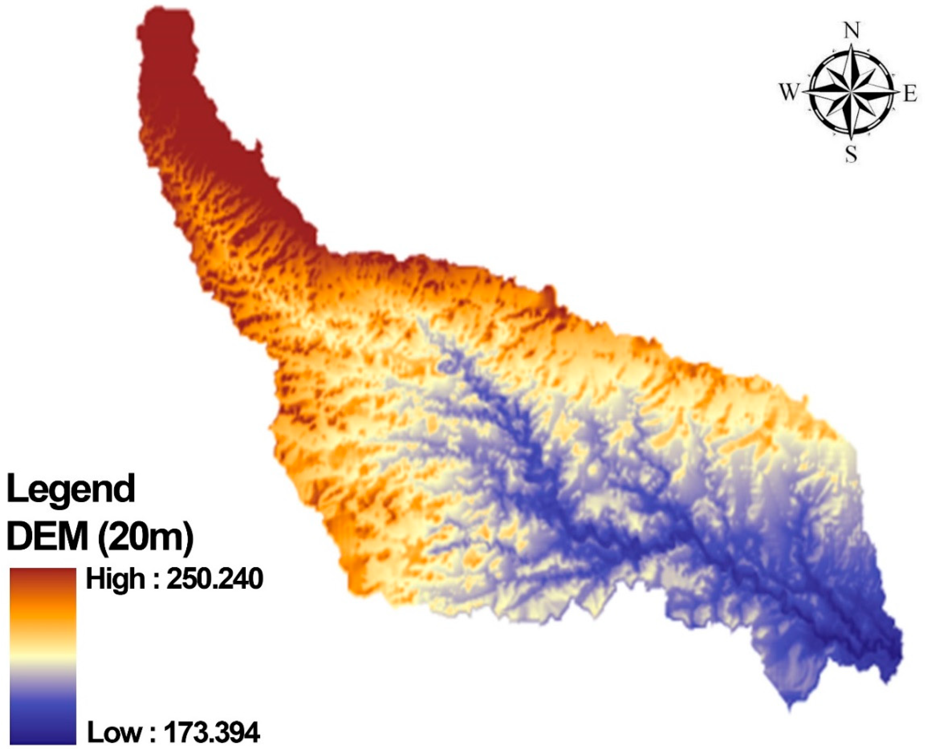
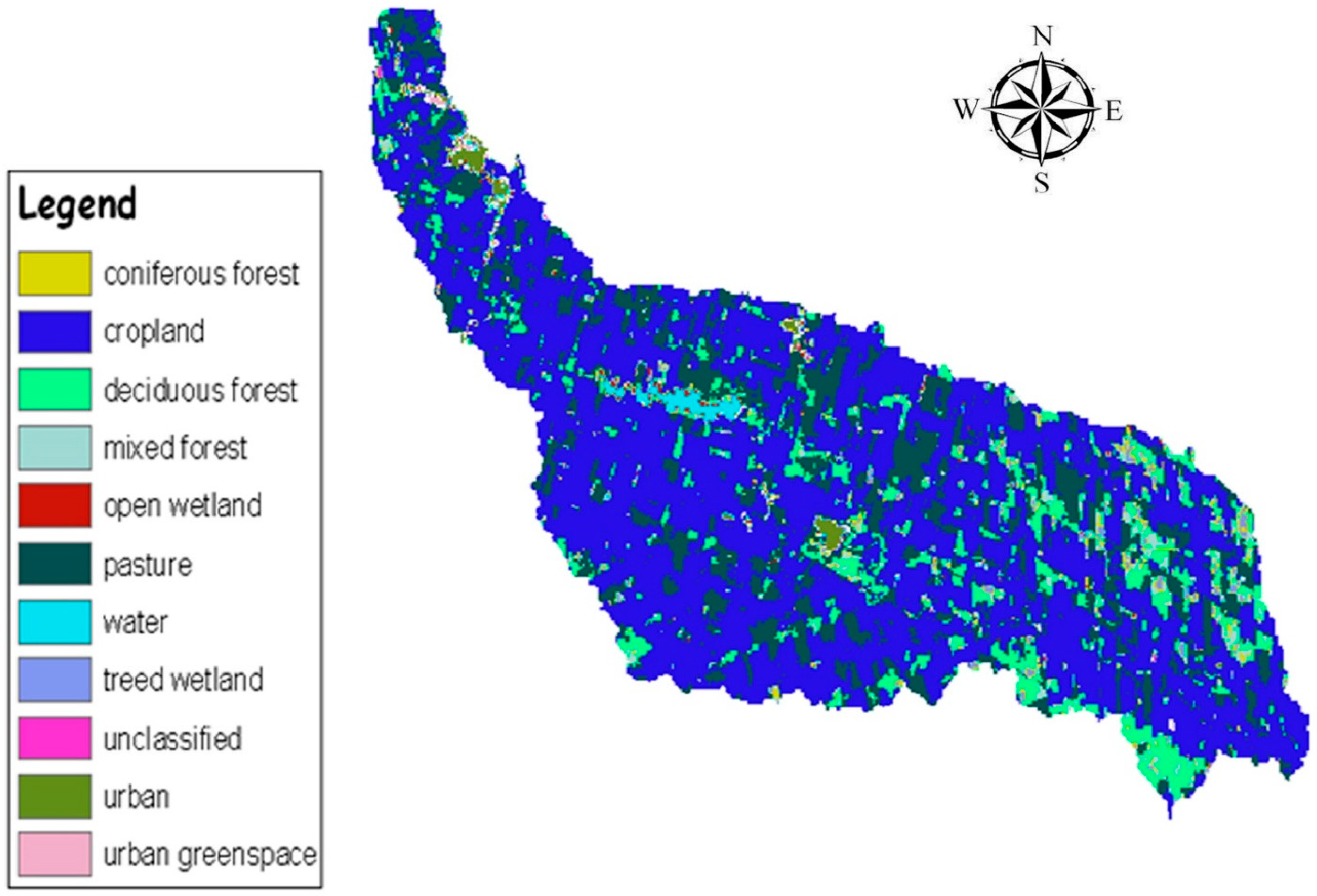
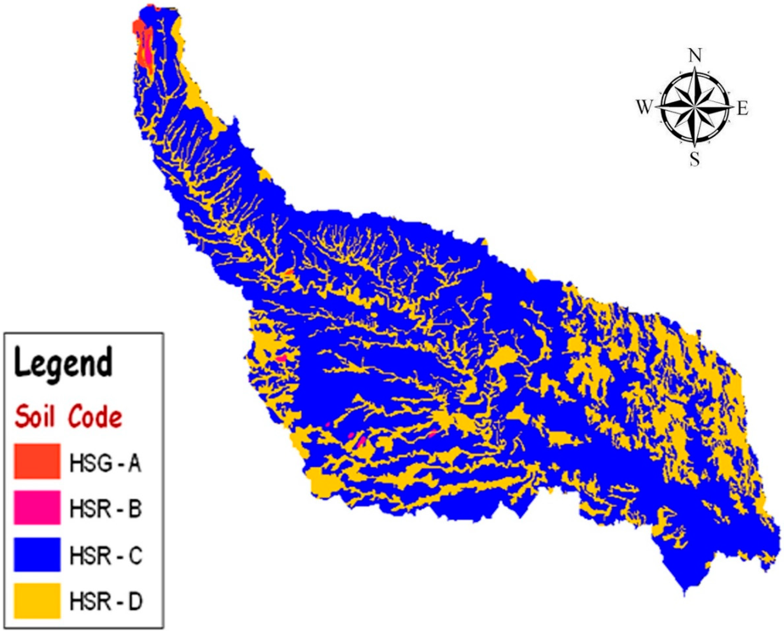
The other details available in Geographical Information System (GIS) layers include 10 m Digital Elevation Model (DEM) (Figure 3), stream network, land use (Figure 4), and soil type (Figure 5). This information was provided by the Ontario Ministry of Natural Resources (MNR), Ontario Ministry of Agriculture, Food and Rural Affairs (OMAFRA), and NPCA. The dominant Hydrologic Soil Groups (HSGs) are type C and D, and approximately 85% of the land is under crop and other agricultural use.

2.2. Rainfall Data

The rain gauge at Hamilton Airport (Climate ID: 6153194) is the only gauge located in the Upper Welland River Watershed. For modeling needs, the Inverse Distance Weighted (IDW) interpolation method was used with data from three other rain gauges in the vicinity to capture the spatial variability of rainfall events. The radar rainfall data were obtained from NEXRAD in Buffalo Radar Station at Buffalo, New York, NY, USA. The watershed is approximately 150 km from the Buffalo Radar station. The GIS-based Digital Precipitation Array (DPA) product contained the precipitation accumulation in a 131 × 131 array of grid boxes at a grid resolution of approximately 4 km × 4 km. Radar captures the DPA rainfall values every 5 min during rainfall periods and every 6–10 min during non-rainfall periods.

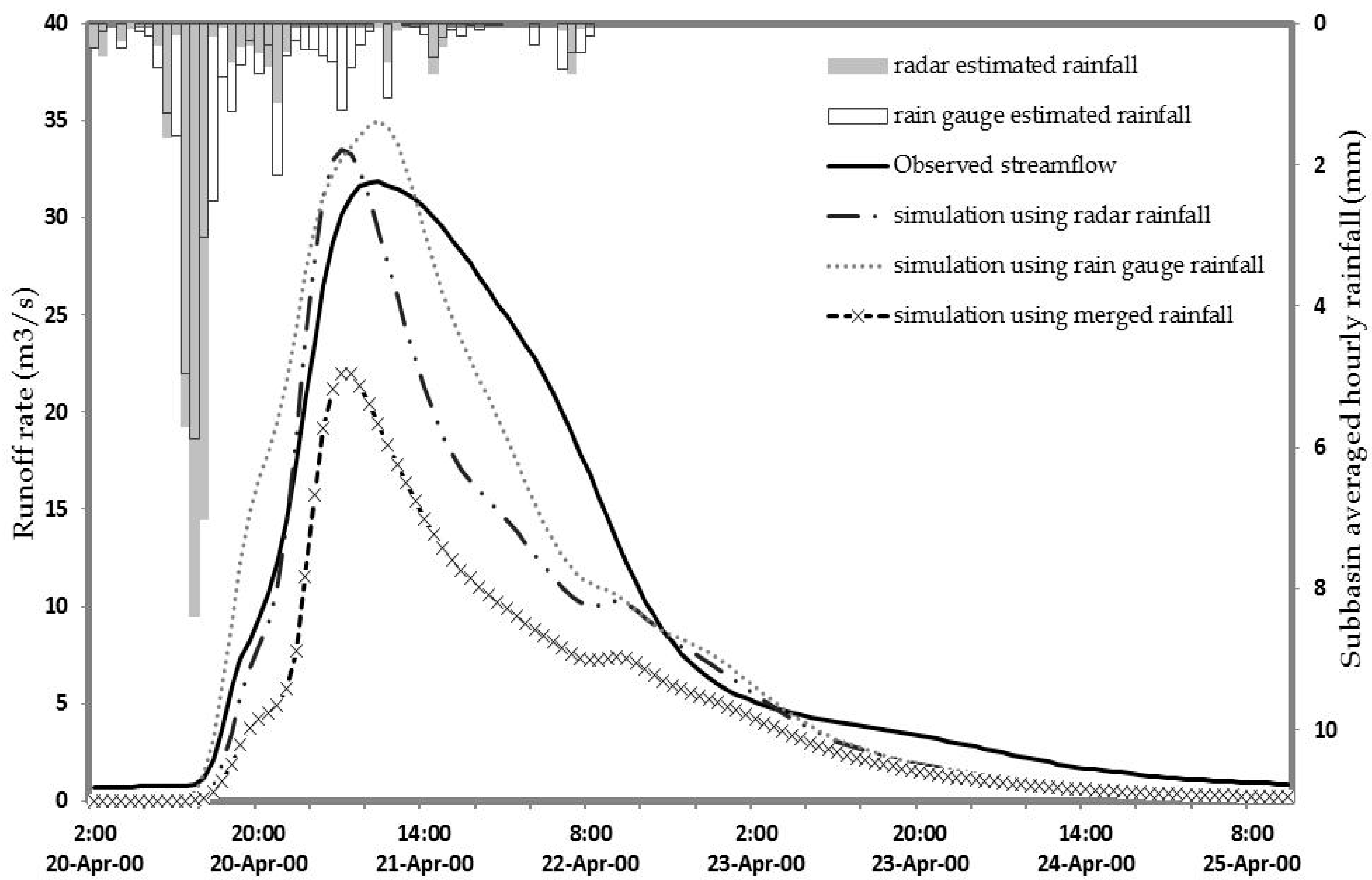
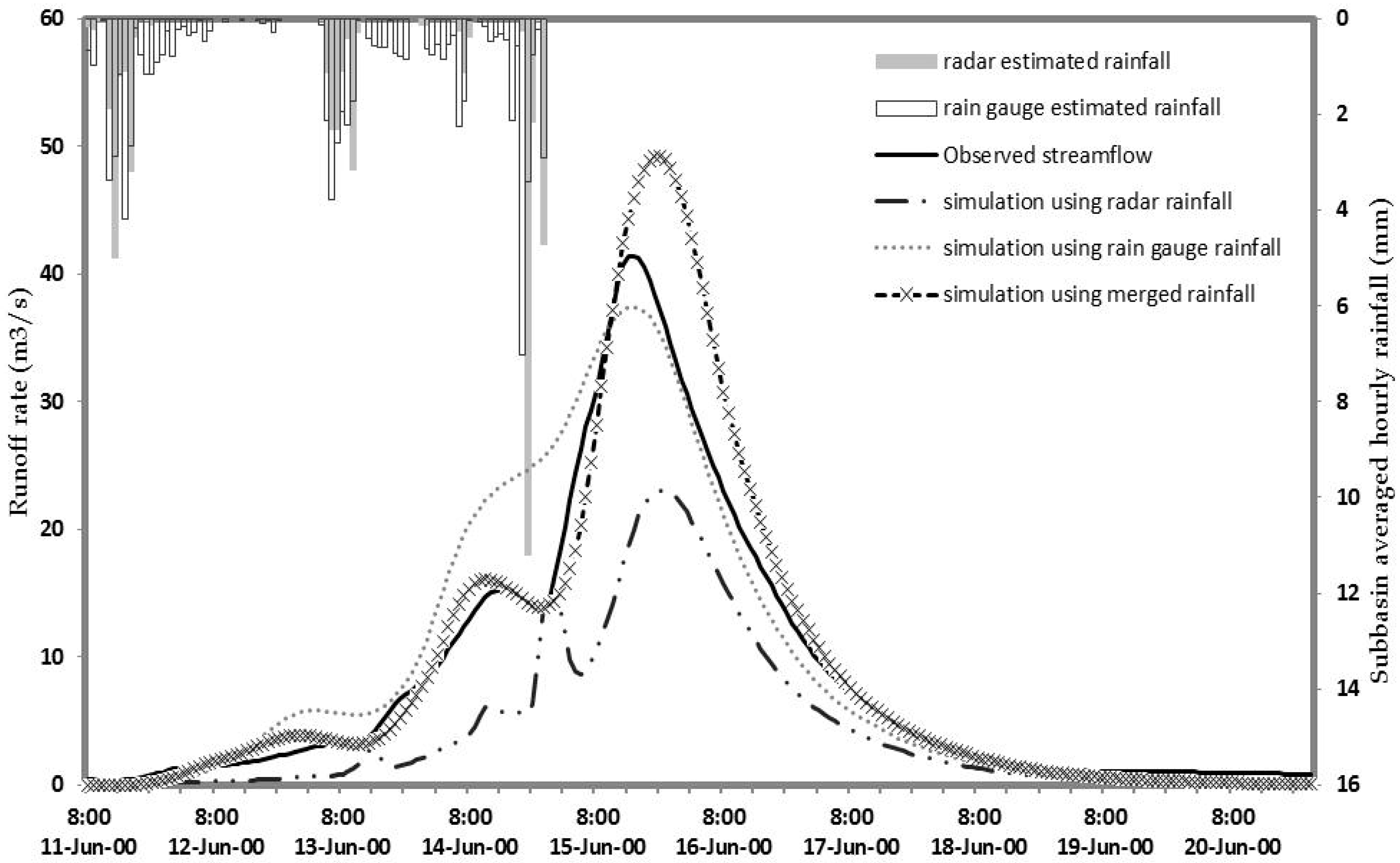
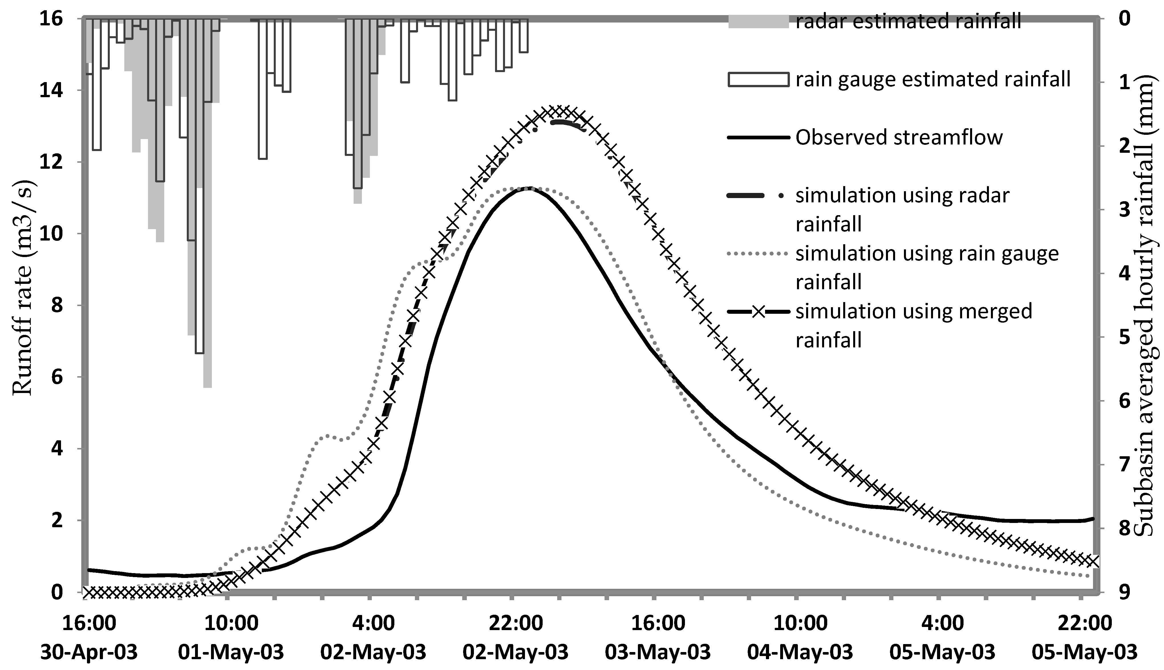
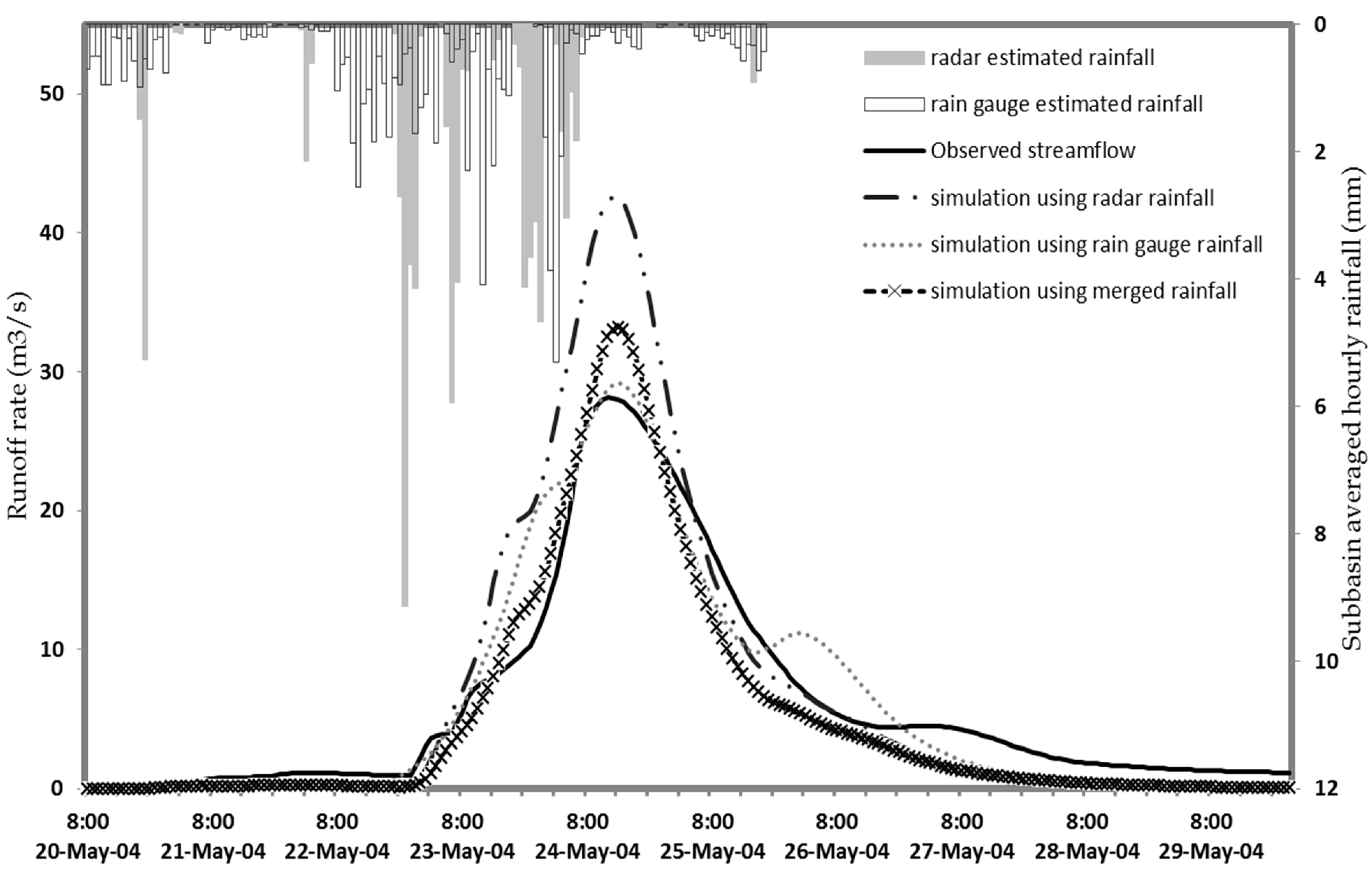
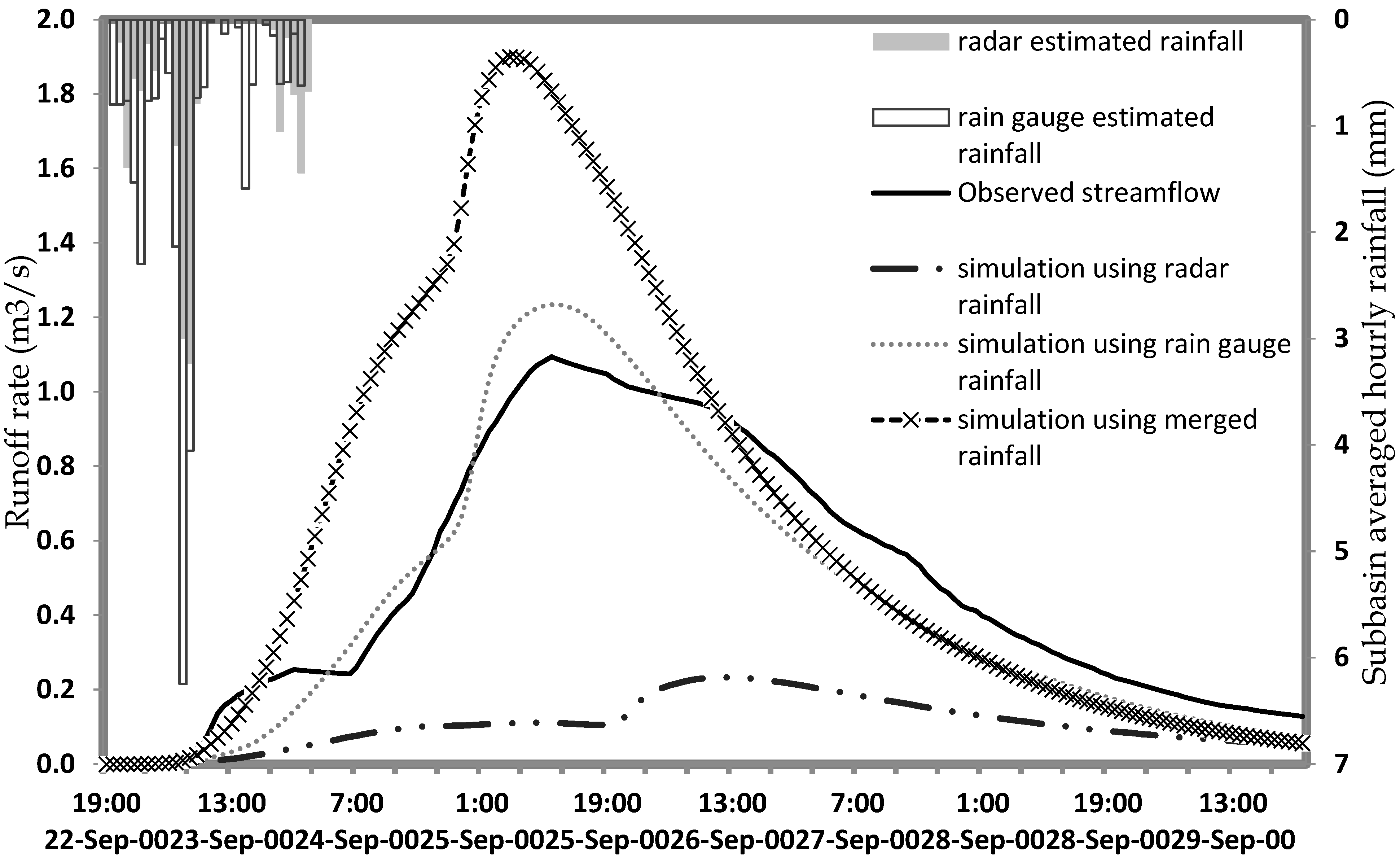
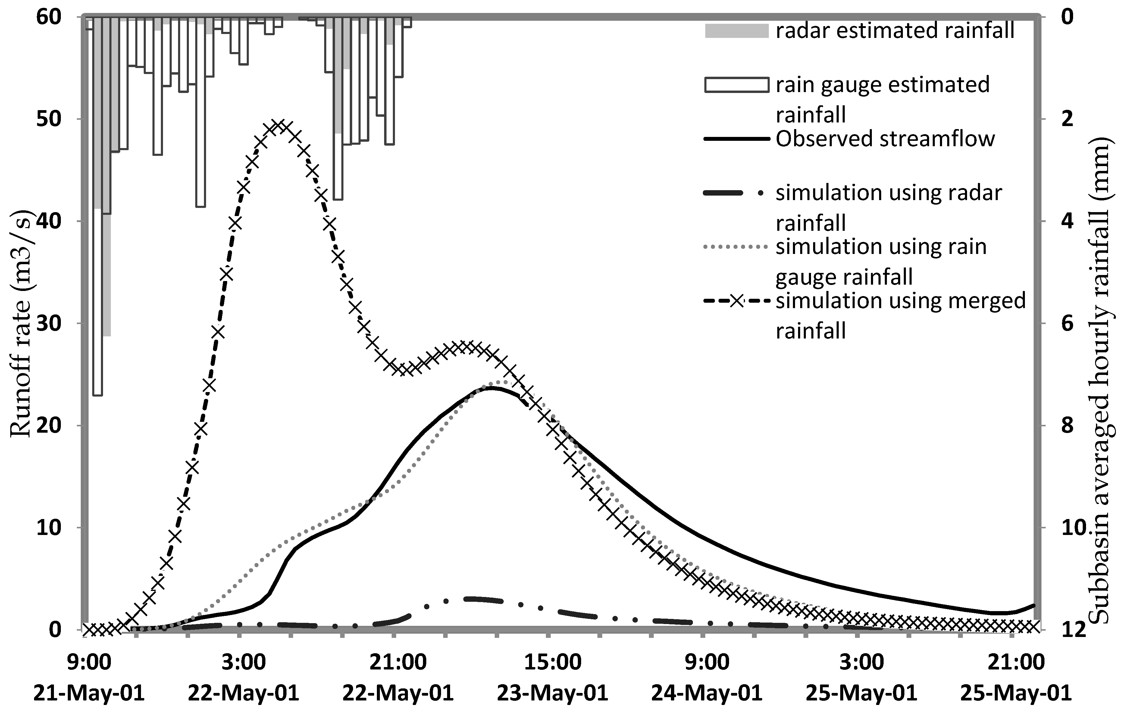
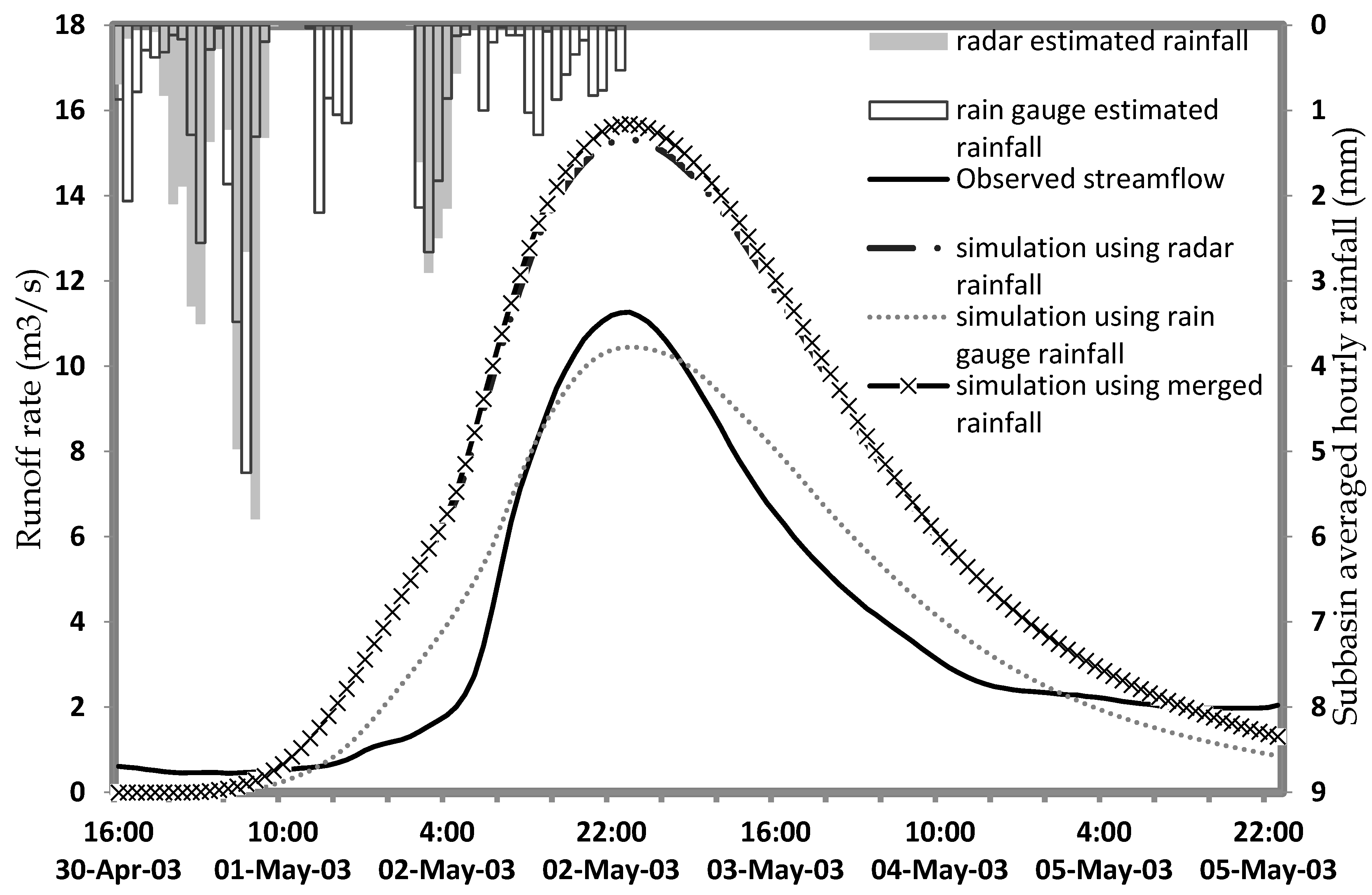
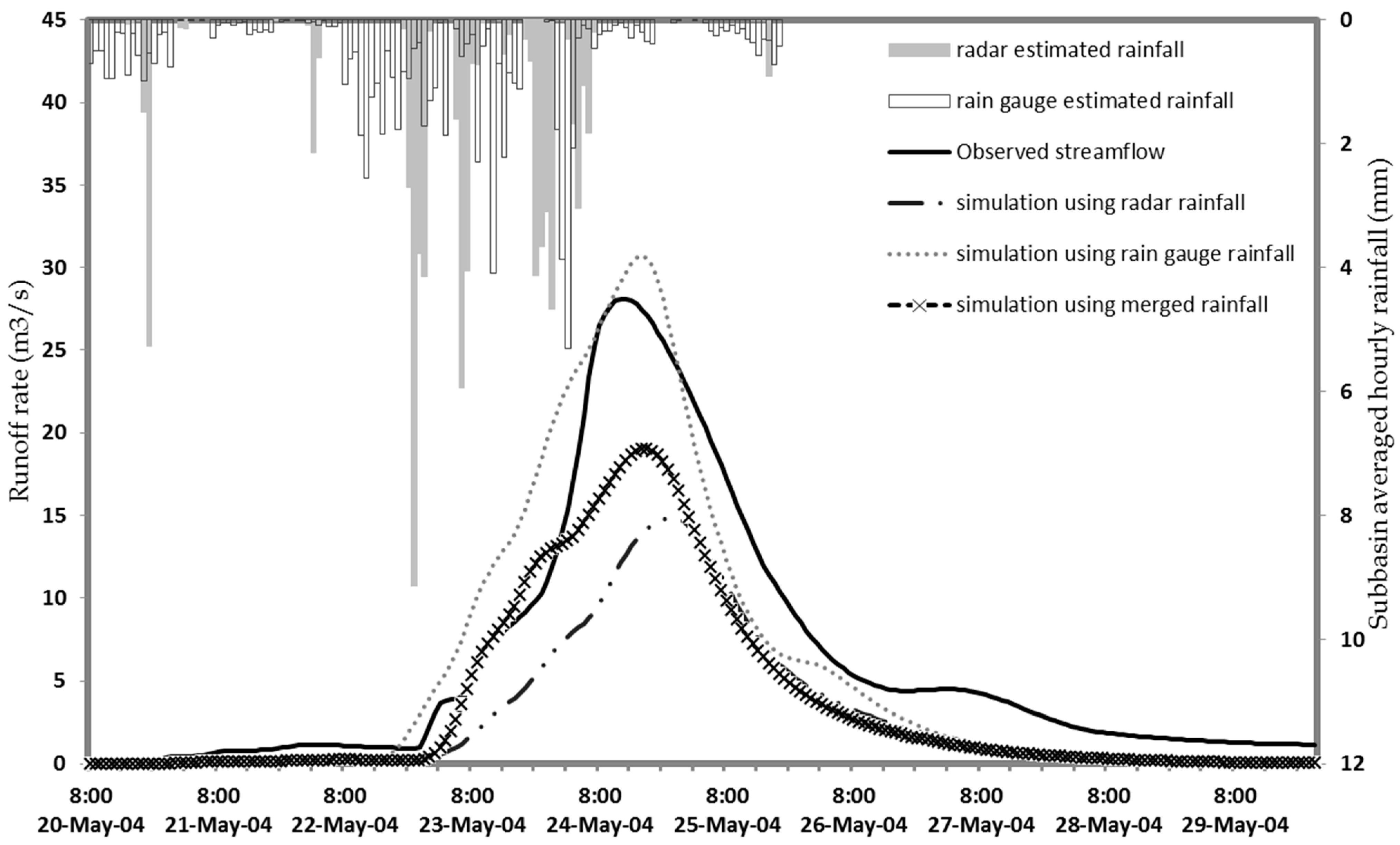
2.3. Selection of Runoff Events

Ten rainfall events were selected from a 5-year database (2000–2004) in order to compare the simulated streamflow with the observed streamflow. The main criteria used for the selection of events included the rainfall precipitation that spatially covers the entire watershed, along with the measurable runoff amount, the availability of rainfall, and the observed streamflow data. To avoid the complexity of modeling Canada’s melting snow and areal snow distribution, the snowfall events were not included in the analysis. The rainfall characteristics of nine runoff events are summarized in

Table 1. Summary of rainfall characteristics for the nine rainfall events used in this study.

Start Time	End Time	Rainfall	Rainfall Volume (mm)		% Difference
		Duration (h)	Rain Gauge	Radar
20 April 2000 (2:00)	22 April 2000 (8:00)	55	36.05	30.82	−14.5
11 June 2000 (8:00)	14 June 2000 (23:00)	88	69.9	44.49	−36.4
9 July 2000 (8:00)	9 July 2000 (17:00)	10	26.45	12.6	−52.4
22 September 2000 (19:00)	23 September 2000 (23:00)	29	26.79	15.92	−40.6
21 May 2001 (9:00)	22 May 2001 (22:00)	38	55.32	18.62	−66.3
11 May 2002 (17:00)	14 May 2002 (9:00)	65	43.9	32.31	−26.4
30 April 2003 (16:00)	2 May 2003 (23:00)	56	42.27	39.89	−5.6
2 November 2003 (4:00)	4 November 2003 (16:00)	61	29.62	29.61	0.0
20 May 2004 (8:00)	25 May 2004 (18:00)	131	68.76	69.69	+1.4

.

2.4. Model Selection Criteria

The selection of a suitable hydrological model for the study was based on many factors, such as identifying the modeling task, considering available dataset inputs, required modeling outputs, and possible constraints (e.g., cost and time involved). The criterion for models considered in this event-based simulation study was their ability to simulate individual rainfall–runoff events. In this context, there was an emphasis on infiltration and surface runoff, simulating surface runoff hydrograph (including peak flow, total volume, and time to peak) at the watershed outlet reservoir and channel routing components. In addition, cost, simplicity, and graphical user interface (GUI) were considered for the final selection of the model.

The evaluation of hydrologic models started with 19 famous water quantity hydrologic models. Out of the considered models, only six models were identified as event-based models (HEC-HMS, ANSWERS, AGNPS, KINEROS, MIKE-SHE, and CASD2D) and were evaluated for their inputs, various routines, and outputs. Out of these reviewed models, only HEC-HMS was able to meet the requirement of the potential hydrologic model in accordance with the objectives of this study. AGNPS and KINEROS models are not suitable since they are limited to watersheds of 200 km² and 100 km² areas, respectively. The study area finalized for this research is about 230 km² (Upper Welland River Watershed). The MIKE-SHE model is, without doubt, one of the best models considering its state-of-art modeling environment. However, the high cost of the model, lack of technical support, and intensive physical input data requirement limited the model’s use for this research. ANSWERS or CASC2D could not be considered since the models lack reservoir routing.

The HEC-HMS model was selected for this study due to its vast applicability in rural and agricultural watersheds in North American conditions and its receptiveness for various hydrological modeling processes (i.e., rainfall excess, runoff hydrograph, base flow, evapotranspiration, channel routing, and reservoir routing). The key advantages of the HEC-HMS model are its sophisticated modeling interface, both empirical and physical-based modeling approaches, lower data requirement, and its availability for extensive documentation and technical support.

2.5. Estimation of Model Parameters

The estimation of model parameters for event-based hydrological models is a critical step due to the uncertainty of estimating the initial soil moisture conditions. The initial input values obtained from field data and/or GIS databases and the literature were used for the first run of the event model. Some of the parameters such as average slope, sub basin area, length of stream channels, imperviousness, and hydraulic conductivity were directly estimated based on the watershed’s physical characteristics. Other parameters were estimated or calibrated during later stages (e.g., time of concentration, curve number, initial moisture, initial abstraction).

2.6. Sensitivity Analysis

The sensitivity analysis helps in identifying the parameters that have a larger impact on the model output response. It provides a valuable insight about the role of each input parameter in relation to the other parameters and the model results. In this study, a simple “local” sensitivity analysis approach has been used for the HEC-HMS model where model results are recorded by incrementing or decrementing each parameter by a given percentage while leaving all others constant and quantifying the change in output values. The selection of the baseline values is important and was obtained from field data and/or GIS databases and the literature for the first run of the event model. These initial parameter values were adjusted based on a graphical comparison of simulated and observed flow hydrographs.

Initial parameter values were adjusted based on the graphical comparison of simulated and observed flow hydrographs. This visual adjustment provides a crude model calibration of manual and automated models within the permissible parameter range of the hydrograph. Then, the model was run repeatedly with the starting baseline values for each parameter, incrementing or decrementing the value by ±5% to ±25%, while keeping all other parameters constant at their nominal starting values.

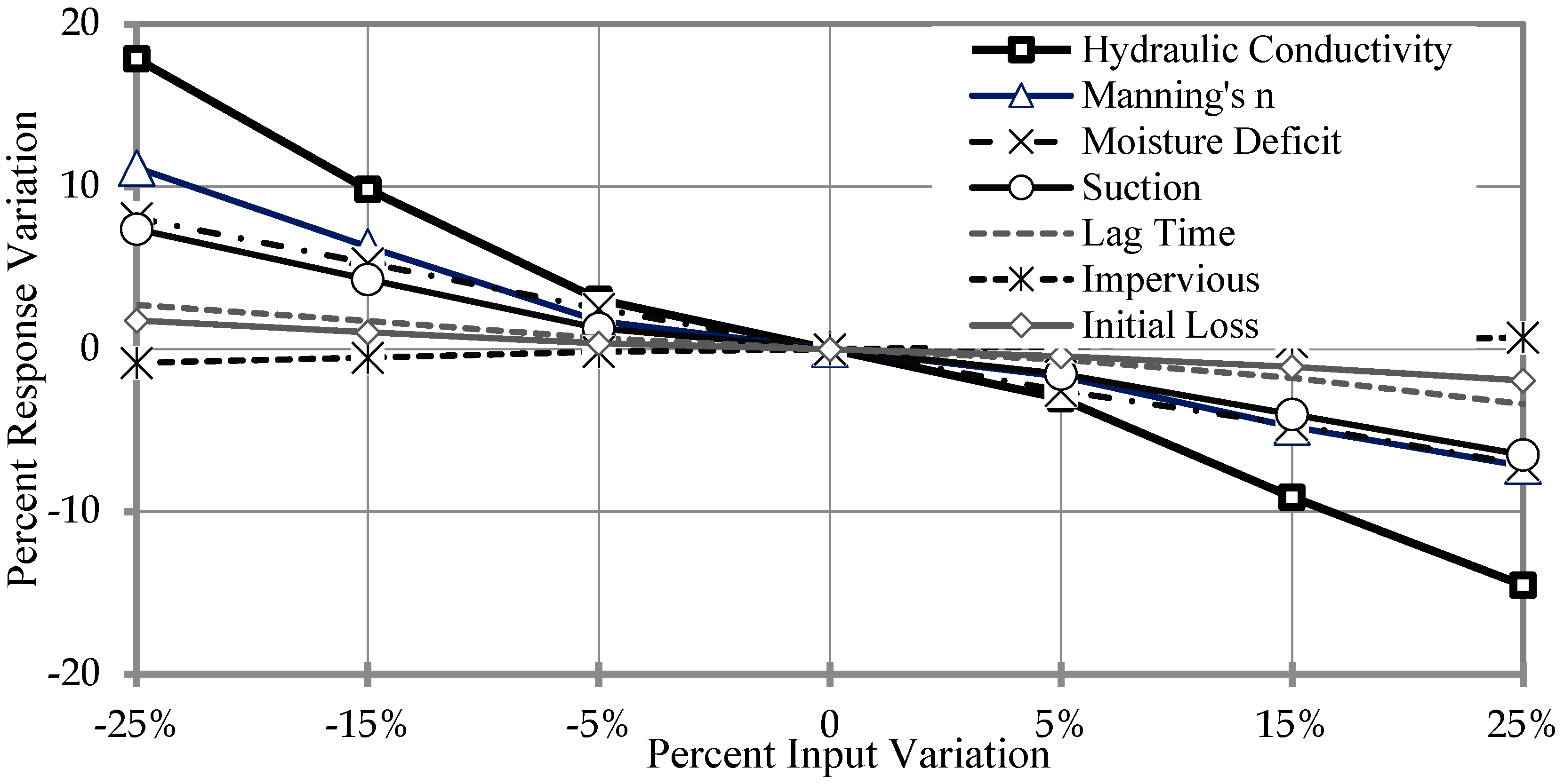
The model was run repeatedly with the starting baseline values for each parameter, incrementing or decrementing the value by ±5%, ±15%, and ±25%. The graphs were plotted using percentage variations in input variables to percentage variations in runoff responses for each parameter to identify the sensitive parameters. The 20 May 2004 event was selected since it was the longest uniformly distributed runoff-event, and moreover, it had parameter values in the mean range. For other events (e.g., 20 April 2000), the curve number either exceeded the permissible range of 100 from its original calculated value when incremented by 15% and 25%, or vice versa (e.g., 22 September 2000). The graphs were plotted using the percentage variations in variable inputs and the percentage variations in runoff responses for each parameter. The plotted graphs were utilized to identify the sensitive parameters.

Figure 6,Figure 7 and Figure 8 show the sensitivity analysis results obtained within ±5%, ±15%, and ±25% variation from the base values. The curve number is the most sensitive parameter at 25% variation from the baseline value. This is probably because of its direct relationship to runoff with the SCS method. When the runoff amount is considered, the Green and Ampt’s hydraulic conductivity is the most sensitive parameter. This is followed by Manning’s roughness coefficient, moisture deficit, and suction at the wetting front. All of these parameters are inversely correlated to runoff volume.

Based on the literature and HEC-HMS technical manual guide (USACE, 2000), the following input parameters were identified for the sensitivity test: initial abstraction and curve number (SCS Loss Method), lag time (SCS Unit Hydrograph), moisture deficit, hydraulic conductivity, impervious percent, suction at wetting front (Green and Ampt loss), and Manning’s roughness coefficient (Muskingum–Cunge routing). These parameters varied in their range of probable values, and thus, the absolute effects of different input parameters were compared. The mode outputs—i.e., runoff amount and peak flow—were selected as the objective functions for the comparison purposes.

The SCS curve number (CN) method [54] is a widely used empirical parameter approach, used in this study to determine the approximate amount of direct runoff from a rainfall event. The runoff curve numbers are based on the hydrologic soil group, land use treatment, and hydrologic condition of the area. The estimation procedure is discussed in detail in the National Engineering Hydrology—NEH-4 handbook [54]. The SCS Unit Hydrograph method was selected to simulate the surface runoff hydrographs. It is based on the dimensionless unit hydrograph approach, developed by Victor Mockus in the 1950s, and is described in detail in the SCS Technical Report [54,55,56].

The other modeling option used in this study is the Green and Ampt Infiltration method [57], a physical parameter approach that functions with the soil suction head, porosity, hydraulic conductivity, and time. These parameters were estimated using GIS-based soil and land use information and previous NPCA reports [58,59,60,61].

The Muskingum–Cunge routing method can be applied to estimate parameters when observed data are missing or the measured flow data have a significant degree of uncertainty [62]. Therefore, the Muskingum–Cunge routing concept was used for channel routing, and the channel geometry was obtained from previous NPCA reports. The roughness coefficient values were also estimated by the Muskingum–Cunge routing method based on [63,64]. The channel side-slope and channel length were computed using GIS elevation data and stream network information.

2.7. Calibration of Model Parameters

Both manual and automated calibration options were used to achieve adequate modeling outputs. The manual calibration was done to identify the sensitive input parameters, followed by the automatic calibration of the identified parameters to refine the model parameter values. First, an adjustment in the time it takes to affect the runoff volume was calibrated, followed by an adjustment in parameters affecting the peak flow, and then an adjustment in the time it takes for events to the peak.

The calibrated parameters were separately computed using rainfall inputs from the rain gauge and radar. These estimated parameters were then compared with each other and in accordance with the antecedent watershed conditions to estimate the suitable set of input parameters. The calibrated parameters were then used to simulate the event streamflow using radar and rain gauge rainfall inputs separately, and these were then compared with observed streamflow.

The SCS unit hydrograph method’s lag time and Green and Ampt method’s initial parameter losses are least sensitive to runoff volume. In addition, the impervious percent area is the only factor, other than the curve number, that is positively correlated to runoff. The peak flow rate was most sensitive to hydraulic conductivity, followed by moisture deficit and suction at the wetting front, and least sensitive to lag time and initial parameter loss.

For this study, the percentage of impervious land has been predicted using the Southern Ontario Land Resource Information System (SOLRIS). Other Green and Ampt parameters such as hydraulic conductivity, moisture deficit, and suction at the wetting front were estimated based on available literature values.

Though curve number values were estimated using the water-balance approach, they were adjusted to minimize the simulation errors in streamflow prediction. The calibration of model parameters explained in the following sections was done based on this sensitivity analysis.

2.8. Evaluation Criteria

A comprehensive comparison of the simulated and observed response requires graphical and statistical approaches [65]. Many graphical and statistical approaches have been used for the evaluation of hydrologic models. Refsgaard et al. [66] recommended using more than one criterion to avoid unrealistic parameter values and poor simulation results. Green and Stephenson [67] presented a list of 21 criteria for single-event simulation models and concluded that no single criterion is sufficient to assess the overall measure of best fit between a computed and an observed hydrograph. In this study, the following criteria (Equations (1)–(4)) were used to assess the goodness-of-fit of the computed hydrographs:

• Percent Error in Peak (PEP) for the comparison of peak flow rates:

$$PEP=\left(\frac{Q_S-Q_O}{Q_O}\right)\times 100$$

(1)

2.

Percent Error in Volume (PEV) for volumetric assessments:

$$PEV=\left(\frac{V_S-V_O}{V_O}\right)\times 100$$

(2)

3.

Percent Error in Time to Peak (PET_P) for accounting time errors:

$$PE{T}_P=\left(\frac{T_S-T_O}{T_O}\right)\times 100$$

(3)

4.

Sum of Squared Residuals (SSR) for assessing the overall goodness-of-fit or shape of a simulated hydrograph:

$$SSR={\sum }_{j=1}^m{\left\{{\sum }_{i=1}^n{\left[Q_O\left(t\right)-Q_S\left(t\right)\right]}^2{}_i\right\}}_j$$

(4)

where m = number of events,

n = number of pairs of ordinates compared in a single event,

$Q_O\left(t\right)$ = observed flow rate at time t,

$Q_S\left(t\right)$ = simulated flow rate at time t,

$V_O$ = observed volume,

$V_S$ = simulated volume,

$T_O$ = observed time to peak,

$T_S$ = simulated time to peak for an event.

The strength of rain gauges to accurately measure rainfall amounts at a single point location is also the weakness of radar rainfall data. On the other hand, the strength of the radars to successfully capture the spatial rainfall pattern is the weakness of the rain gauge rainfall. Consequently, the integration of rain gauge and radar rainfall data can be a suitable solution to the shortcomings of each rainfall method. The Mean Field Bias (MFB) coefficient was computed for each storm event by dividing the total rain gauge rainfall by the total radar rainfall during each event (Equation (5)):

$$MFB=\frac{{\displaystyle \sum _{i=1}^n{G}_i}}{{\displaystyle \sum _{i=1}^n{R}_i}}$$

(5)

where G_i and R_i are corresponding rain gauge and radar rainfall values for the ith hour, respectively, and n is the number of hours during the storm event. This MFB coefficient was multiplied with the radar rainfall datasets to obtain the MFB corrected radar rainfall (or merged radar rainfall).

The Root Mean Squared Error (RMSE) evaluates the goodness of fit by measuring the differences between rain gauge and radar rainfall data [68] and is computed as shown in Equation (6):

$$RMSE=\sqrt{\frac{1}{n}{\displaystyle \sum _{i=1}^n{(r_i-a_i)}^2}}$$

(6)

where n = total number of comparison pairs,

r_i = rain gauge rainfall values,

a_i = radar rainfall values, and

$\stackrel{-}{r}$ and $\stackrel{-}{a}$ represent mean rain gauge and radar values, respectively.

The comparisons between observed and simulated runoff hydrographs with all three inputs (rain gauge, radar, and merge data) using SCS and Green and Ampt outputs were also compared statistically with the coefficient of determination (R²) [69], Nash–Sutcliffe Efficiency (NSE) [70], RMSE observations standard deviation ratio (RSR) [68,71,72], and the PBIAS [73] methods, which explain in detail the overestimation or underestimation of a model. These methods are mentioned in Equations (7)–(10) for reference.

$$R^2=\frac{n[{\sum }_{i=1}^n\left(Y_i{}^{obs}\ast Y_i{}^{sim}\right)]-[{\sum }_{i=1}^n\left(Y_i{}^{obs}\right)\ast {\sum }_{i=1}^n\left(Y_i{}^{sim}\right)]}{\sqrt{\left[n{\sum }_{i=1}^n{(Y_i{}^{obs})}^2-{({\sum }_{i=1}^n(Y_i{}^{obs}))}^2\right]\left[n{\sum }_{i=1}^n{(Y_i{}^{sim})}^2-{({\sum }_{i=1}^n(Y_i{}^{sim}))}^2\right]}}$$

(7)

$$NSE=1-\left[\frac{{\sum }_{i=1}^n{\left(Y_i{}^{obs}-Y_i{}^{sim}\right)}^2}{{\sum }_{i=1}^n{\left(Y_i{}^{obs}-Y^{mean}\right)}^2}\right]$$

(8)

$$RSR=\frac{RMSE}{STDE{V}_{obs}}=\frac{\left[\sqrt{{\sum }_{i=1}^n{\left(Y_i{}^{obs}-Y_i{}^{sim}\right)}^2}\right]}{\left[\sqrt{{\sum }_{i=1}^n{\left(Y_i{}^{obs}-Y^{mean}\right)}^2}\right]}$$

(9)

$$PBIAS=\left[\frac{{\sum }_{i=1}^n\left(Y_i{}^{obs}-Y_i{}^{sim}\right)\ast \left(100\right)}{{\sum }_{i=1}^n\left(Y_i{}^{obs}\right)}\right]$$

(10)

where Y_i ^obs = ith observation for the constituent being evaluated,

Y_i ^sim = ith simulated value for the constituent being evaluated,

Y_mean = mean of observed data for the constituent being evaluated,

n = total number of observations.

R² describes the proportion of the variance in measured data explained by the model (Equation (7)). The range of R² varies from 0 to 1, where values closer to 1 (more than 0.5) are considered as good and acceptable, showing less variability with the measured data.

The Nash–Sutcliffe efficiency (NSE) is a normalized statistic that defines the relative magnitude of the residual variance when compared to the observed data variance (Equation (8)). The range of NSE values varies between −∞ and 1; however, values between 0 and 1 are generally classified as acceptable performance for the model. Values less than 0 show the poor performance of the simulation model.

Another model evaluation statistic, named the RMSE observations standard deviation ratio (RSR), developed and recommended by [68,71], was also used to compare the observed and simulated data for the study. In addition, RSR normalizes the RMSE by taking into account the observed standard deviation, as the literature recommended [72]. Equation 9 shows that RSR is calculated as the ratio of the RMSE and standard deviation of measured data.

Percent bias (PBIAS) (Equation (10)) tells as a percentage the deviation of data that are estimated to the observed data. The maximum value for PBIAS is 0.0; however, values closer to zero are considered good. In addition, positive and negative values show the underestimation and overestimation biases, respectively, for the performance of the model.

3. Results and Discussion

Two runoff estimation options available in the HEC-HMS were used when evaluating the use of rainfall data obtained by rain gauges and radar. First, the results obtained using the SCS model are presented and discussed in Section 3.1, followed by those obtained using the Green and Ampt Infiltration approach, which are discussed in Section 3.2. The HEC-HMS model was initially run with the best-estimated model parameters and then with the calibrated event-dependent parameters for each event.

3.1. SCS Runoff Model

The comparison between simulated and observed peak flow rate, runoff amount, and time to peak using the best estimated SCS model parameters with rainfall data and percentage error difference are summarized in

Table 2. Summary of observed and simulated peak flow rate, runoff amount, and time to peak obtained using best estimated SCS model parameters with rain gauge and radar rainfall inputs.

Event	Observed Stream Flow Results			Simulated Results Using Rain Gauge Rainfall			Simulated Results Using Radar Rainfall
	Peak Flow Rate (m3/s)	Runoff Amount (mm)	Time to Peak (h)	Peak Flow Rate (m3/s)	Runoff Amount (mm)	Time to Peak (h)	Peak Flow Rate (m3/s)	Runoff Amount (mm)	Time to Peak (h)
20-04-2000	31.85	19.45	32	41.71	22.49	32	41.01	18.87	30
11-06-2000	41.42	31.07	104	58.04	50.51	95	55.6	28.65	98
09-07-2000	3.95	3.26	43	6.73	4.05	39	0.45	0.40	15
22-09-2000	1.09	1.32	65	0.62	0.51	57	0.31	0.3	66
21-05-2001	23.67	15.05	48	59.91	34.79	40	10.51	5.96	37
11-05-2002	26.38	18.54	63	51.45	32.02	65	48.38	21.17	62
30-04-2003	11.27	7.63	57	19.19	14.74	41	22.48	13.70	43
02-11-2003	13.83	13.83	38	1.95	1.42	86	2.05	1.78	55
20-05-2004	28.11	22.36	101	44.36	44.33	109	58.89	48.33	110

and

Table 3. Statistical comparison between observed and simulated peak flow rate, runoff amount, and time to peak using best estimated SCS model parameters.

Event	% Error in Peak Flow		% Error in Runoff Amount		% Error in Time to Peak
	Rain Gauge	Radar	Rain Gauge	Radar	Rain Gauge	Radar
20-04-2000	31	28.8	15.6	−3.0	0.0	−6.3
11-06-2000	40.1	34.2	62.6	−7.8	−8.7	−5.8
09-07-2000	70.4	−88.6	24.2	−87.7	−9.3	−65.1
22-09-2000	−43.1	−71.6	−61.4	−77.3	−12.3	1.5
21-05-2001	153.1	−55.6	131.2	−60.4	−16.7	−22.9
11-05-2002	95	83.4	72.7	14.2	3.2	−1.6
30-04-2003	70.3	99.5	93.2	79.6	−28.1	−24.6
02-11-2003	−85.9	−85.2	−89.7	−87.1	126.3	44.7
20-05-2004	57.8	109.5	98.3	116.1	7.9	8.9
Average	43	6	39	−13	7	−8

, respectively. Comparing the simulated peak flow rate and runoff amount with the observed peak flow rate and runoff amount results in an overestimation for most of the events. In addition, the simulated time to peak, either using a rain gauge or radar data, was less than the observed time to peak (Table 2).

The percentage error difference for the simulated peak flow rate using rain gauge data varied from +153% to −85% compared with the observed peak flow rates for the individual rainfall events. The average percentage error differences of 43.2% and 38.5% for peak flow rate were found with rainfall obtained by rain gauge and radar rainfall inputs, respectively (Table 3). However, the analysis for runoff amount showed a very low average percentage error difference between the simulated (area under the hydrograph) and the observed hydrographs—approximately 6% with radar rainfall and 6.9% with rain gauge rainfall. The difference between the simulated and observed average time to peak showed less time for the simulated (−12.6 and −7.9% with rain gauge and radar rainfall data, respectively) rainfall events. Since both sources of rainfall inputs provided a high range of errors for peak runoff rate in simulated modeling outputs, and the model parameters were therefore calibrated to represent the event-dependent antecedent’s watershed conditions.

The modeling results obtained using the calibrated SCS model parameters are summarized in

Table 4. Summary of observed and simulated peak flow rate, runoff amount, and time to peak obtained using calibrated SCS model parameters with rain gauge and radar rainfall inputs.

Event	Observed Stream Flow Data			Using Rain Gauge Rainfall			Using Radar Rainfall
	Peak Flow Rate (m3/s)	Runoff Amount (mm)	Time to Peak (h)	Peak Flow Rate (m3/s)	Runoff Amount (mm)	Time to Peak (h)	Peak Flow Rate (m3/s)	Runoff Amount (mm)	Time to Peak (h)
20-04-2000	31.85	19.45	32	34.99	18.28	32	33.54	15.07	28
11-06-2000	41.42	31.07	104	37.43	33.45	104	23.08	15.94	109
09-07-2000	3.95	3.26	43	4.83	2.98	42	0.26	0.25	64
22-09-2000	1.09	1.32	65	1.37	1.2	65	0.26	0.3	78
21-05-2001	23.67	15.05	48	26.22	13.68	48	0.94	0.56	70
11-05-2002	26.38	18.54	63	16.73	16.73	63	24.06	9.11	60
30-04-2003	11.27	7.63	57	11.25	8.14	55	13.12	9.7	61
02-11-2003	13.83	13.83	38	17.3	10.54	41	24.89	10.91	18
20-05-2004	28.11	22.36	101	29.2	22.26	101	42.6	25.38	100

and

Table 5. Statistical comparison between observed and simulated peak flow rate, runoff amount, and time to peak using calibrated SCS model parameters.

Event	% Error in Peak Flow		% Error in Runoff Amount		% Error in Time to Peak
	Rain Gauge	Radar	Rain Gauge	Radar	Rain Gauge	Radar
20-04-2000	9.9	5.3	−6.0	−22.5	0.0	−12.5
11-06-2000	−9.6	−44.3	7.7	−48.7	0.0	4.8
09-07-2000	22.3	−93.4	−8.6	−92.3	−2.3	48.8
22-09-2000	25.7	−76.1	−9.1	−77.3	0.0	20.0
21-05-2001	10.8	−96.0	−9.1	−96.3	0.0	45.8
11-05-2002	−36.6	−8.8	−9.8	−50.9	0.0	−4.8
30-04-2003	−0.2	16.4	6.7	27.1	−3.5	7.0
02-11-2003	25.1	80.0	−23.8	−21.1	7.9	−52.6
20-05-2004	3.9	51.5	−0.4	13.5	0.0	−1.0
Average	6	−19	−6	−41	0.0	6

. These results indicate that using both data inputs, with the calibrated SCS inputs, simulated streamflows were close to the observed values. When rain gauge inputs had less time to peak, the runoff amount was simulated better when compared with the observed data. The range of the percentage error difference reduced significantly (−36.6 to +25.7%) (Table 5) compared with the best-estimated results presented in Table 3. In addition, the analysis in terms of the average percentage error difference showed an approximately 6% difference with rain gauge and −19% with radar inputs when compared with the observed peak flow rate (Table 5).

The average percentage error difference for runoff amount using simulated rain gauge data was less than 6%; however, the simulated radar data showed a value of −41% when estimating the surface runoff amount. The average percentage error in time to peak showed almost no difference when estimated with rain gauge inputs; however, there was a 6% overestimation using radar data inputs compared to the observed time to peak. Overall, there was a major improvement in simulated and observed values when the calibrated set of parameters was used with rain gauge and radar rainfall inputs. However, the fractional percentage error in radar simulated modeling results was relatively higher when compared with observed streamflow using calibrated parameters.

3.2. Green and Ampt Infiltration Model

The other option available (the physically based Green and Ampt infiltration method) was also used to simulate streamflow, using rainfall obtained from rain gauge and radar data. The results were obtained with the best-estimated model parameters, and the rainfall inputs from rain gauge and radar are summarized in

Table 6. Summary of observed and simulated peak flow rate, runoff amount, and time to peak obtained using best estimated Green and Ampt model parameters with rain gauge and radar rainfall inputs.

Event	Observed Stream Flow Data			Using Rain Gauge Rainfall			Using Radar Rainfall
	Peak Flow rate (m3/s)	Runoff Amount (mm)	Time to Peak (h)	Peak Flow Rate (m3/s)	Runoff Amount (mm)	Time to Peak (h)	Peak Flow Rate (m3/s)	Runoff Amount (mm)	Time to Peak (h)
20-04-2000	31.85	19.45	32	37.78	16.49	27	48.64	19.18	28
11-06-2000	41.42	31.07	104	35.85	35.45	95	54.67	27.77	98
09-07-2000	3.95	3.26	43	12.37	7.25	35	0.99	0.65	24
22-09-2000	1.09	1.32	65	0.54	0.49	64	0.31	0.3	66
21-05-2001	23.67	15.05	48	40.45	31.20	28	21.06	10.50	24
11-05-2002	26.38	18.54	63	23.73	15.69	65	34.69	13.48	61
30-04-2003	11.27	7.63	57	31.28	19.00	33	37.08	21.08	27
02-11-2003	13.83	13.83	38	0.43	0.33	99	2.66	2.18	54
20-05-2004	28.11	22.36	101	25.92	24.10	110	48.09	40.68	106

and

Table 7. Statistical comparison between observed and simulated peak flow rate, runoff amount, and time to peak using best estimated Green and Ampt model parameters.

Event	% Error in Peak Flow		% Error in Runoff Amount		% Error in Time to Peak
	Rain Gauge	Radar	Rain Gauge	Radar	Rain Gauge	Radar
20-04-2000	18.6	52.7	−15.2	−1.4	−15.6	−12.5
11-06-2000	−13.4	32.0	14.1	−10.6	−8.7	−5.8
09-07-2000	213.2	−74.9	122.4	−80.1	−18.6	−44.2
22-09-2000	−50.5	−71.6	−62.9	−77.3	−1.5	1.5
21-05-2001	70.9	−11.0	107.3	−30.2	−41.7	−50.0
11-05-2002	−10.0	31.5	−15.4	−27.3	3.2	−3.2
30-04-2003	177.6	229.0	149.0	176.3	−42.1	−52.6
02-11-2003	−96.9	−80.8	−97.6	−84.2	160.5	42.1
20-05-2004	−7.8	71.1	7.8	81.9	8.9	5.0
Average	34	20	24	−6	5	−14

. Comparing the results given in both tables indicates that the model results obtained using the best estimated parameters with SCS option (Table 2 and Table 3) and Green and Ampt infiltration option (Table 6 and Table 7) are similar. In addition, the percentage error obtained from both rain gauge and radar rainfall inputs simulated results are in the same range as the SCS method and Green and Ampt option. The percentage error difference for peak flow rate ranged from 213.2% to −96.9% with rain gauge and radar rainfall simulated data using the Green and Ampt method (Table 7). The average percentage error values for the peak flow rate were 34% and 20% for rain gauge and radar data inputs, respectively. The percentage differences for the simulated runoff were 24% and −6% with rain gauge and radar data, respectively. The analysis of time to peak showed a smaller % percentage difference with rain gauge (5%) compared to (−14%) with radar data for these rainfall events when compared with the observed values (Table 7).

To reduce the percentage error difference for observed and simulated peak flow rate, runoff amount, and time to peak, the Green and Ampt method parameters were calibrated and again used for simulation as shown in

Table 8. Summary of observed and simulated peak flow rate, runoff amount, and time to peak obtained using calibrated Green and Ampt model parameters with rain gauge and radar rainfall Inputs.

Event	Observed Stream Flow Results			Simulated Results Using Rain Gauge Rainfall			Simulated Results Using Radar Rainfall
	Peak Flow Rate (m3/s)	Runoff Amount (mm)	Time to Peak (h)	Peak Flow Rate (m3/s)	Runoff Amount (mm)	Time to Peak (h)	Peak Flow Rate (m3/s)	Runoff Amount (mm)	Time to Peak (h)
20-04-2000	31.85	19.45	32	34.99	17.51	35	41.04	19.08	35
11-06-2000	41.42	31.07	104	26.7	27.02	106	34.99	20.8	109
09-07-2000	3.95	3.26	43	4.3	3.02	43	0.45	0.37	32
22-09-2000	1.09	1.32	65	1.13	1.18	69	0.23	0.29	90
21-05-2001	23.67	15.05	48	24.27	13.59	49	3	1.33	45
11-05-2002	26.38	18.54	63	29.65	16.65	66	34.44	11.77	62
30-04-2003	11.27	7.63	57	8.18	8.18	57	15.32	12.37	57
02-11-2003	13.83	13.83	38	23	10.4	37	41.67	13.09	16
20-05-2004	28.11	22.36	101	14.84	10.6	113	28.72	20.37	105

and

Table 9. Statistical comparison between observed and simulated peak flow rate, runoff amount, and time to peak using calibrated Green and Ampt model parameters.

Event	% Error in Peak Flow		% Error in Runoff Amount		% Error in Time to Peak
	Rain Gauge	Radar	Rain Gauge	Radar	Rain Gauge	Radar
20-04-2000	9.9	28.9	−10.0	−1.9	9.4	9.4
11-06-2000	−35.5	−15.5	−13.0	−33.1	1.9	4.8
09-07-2000	8.9	−88.6	−7.4	−88.7	0.0	−25.6
22-09-2000	3.7	−78.9	−10.6	−78.0	6.2	38.5
21-05-2001	2.5	−87.3	−9.7	−91.2	2.1	−6.3
11-05-2002	12.4	30.6	−10.2	−36.5	4.8	−1.6
30-04-2003	−27.4	35.9	7.2	62.1	0.0	0.0
02-11-2003	66.3	201.3	−24.8	−5.4	−2.6	−57.9
20-05-2004	−47.2	2.2	−52.6	−8.9	11.9	4.0
Average	−1	3	−5	−31	4	−4

. Table 8 shows that simulated values for all the variables using rain gauge and radar data are similar to the observed values for most rainfall events. This is also evident in the peak flow rate analysis, which has a low average percentage error difference of −1% and −3% for rain gauge and radar inputs, respectively (Table 9). However, the average percentage error for runoff amount using rain gauge and radar data was as large as −5% and −31%, respectively. The simulated results showed better comparison for time to peak with observed data either using the rain gauge data (4%) or the radar data (−4%).

The statistical analysis of the comparison between SCS and Green and Ampt options in terms of the Sum of Square Residuals (SSR) and Root Mean Square Errors (RMSE) is presented in

Table 10. Statistical comparison of modeling results obtained using SCS curve number and Green and Ampt runoff options.

s.no.	Event	SCS Curve Number Option				Green and Ampt Option
		Sum of Square Residuals		Root Mean Square Error		Sum of Square Residuals		Root Mean Square Error
		Rain Gauge	Radar	Rain Gauge	Radar	Rain Gauge	Radar	Rain Gauge	Radar
1	20-04-2000	1291.4	2316.1	3.1	4.2	656.9	1538.5	2.2	3.4
2	11-06-2000	2488	10,661.1	3.3	6.8	4157.1	4461.2	4.2	4.4
3	09-07-2000	58	487.3	0.7	2.1	30.5	445.7	0.5	2
4	22-09-2000	3.1	38.5	0.1	0.5	2	40.6	0.1	0.5
5	21-05-2001	291.3	13,708.6	1.6	11.2	428	12,043.7	2	10.5
6	11-05-2002	1066.6	4185.7	2.5	4.9	1476.5	2940.3	2.9	4.1
7	30-04-2003	324.8	382.3	1.6	1.7	113.2	1298.6	0.9	3.2
8	02-11-2003	945.8	5591.4	2.9	6.9	1280.6	17,284.1	3.3	12.3
9	20-05-2004	1243.6	4486.9	2.3	4.4	1683.9	5694.8	2.7	5
Average		857.0	4650.9	2.0	4.7	1092.1	5083.1	2.1	5.0

. Overall, it seems that the SCS method was able to compute runoff amounts with fewer errors than the Green and Ampt option in the case of both rain gauge and radar rainfall. The rain gauge estimated SSR at 857 mm, which is about six times less than that estimated using the radar rainfall data, at 4650 mm.

The RMSE obtained using the rain gauge rainfall data is about less than half of that estimated using the radar rainfall. This supports the observations in the other analysis that better runoff results were obtained using rain gauge rainfall data for all nine runoff events. A similar trend was noticed with the Green and Ampt modeling option. The estimated rain gauge runoff results show an about five times smaller SSR than radar runoff results and about two times less RMSE error in the case of the Green and Ampt option. The RMSE errors obtained with the rain gauge rainfall were numerically the same with both SCS and Green and Ampt options, but in the case of radar rainfall, the SCS method gave slightly lower errors. Similar results have been reported in past comparison studies between SCS and Green and Ampt options [74].

Although the differences in the errors between these two methods are not large, the SCS method is reasonably appropriate for modeling the runoff at the sub-basin scale, especially for agricultural watersheds such as the Upper Welland River Watershed. Because the Green and Ampt model parameters are physically based and are measured in the field, it is usually thought to be more reliable than the SCS option [75].

Based on the runoff comparison results obtained using both SCS and the Green and Ampt methods, with rain gauge and radar rainfall data, it seems that radar rainfall produced higher errors in runoff simulation. This is because of the erroneous point rainfall estimated using the radar. To make use of the spatial capability of the radar rainfall and the point accuracy of the rain gauge rainfall, the radar rainfall inputs were corrected using the MFB correction factor. These data were used to simulate the peak flow rate, runoff amount, and time to peak for the nine runoff events.

The comparison of the MFB corrected results is presented in

Table 11. Summary of observed and simulated runoff amount, peak flow, and time to peak obtained using calibrated SCS and Green and Ampt Model parameters with MFB-corrected radar rainfall input.

Event	Observed Stream Flow Results			Simulated Results Using			Simulated Results Using
				SCS Curve Number Option			Green and Ampt Option
	Peak Flow Rate (m3/s)	Runoff Amount (mm)	Time to Peak (hr)	Peak Flow Rate (m3/s)	Runoff Amount (mm)	Time to Peak (h)	Peak Flow Rate (m3/s)	Runoff Amount (mm)	Time to Peak (h)
20-04-2000	31.85	19.45	32	21.99	10.09	28	30.49	14.59	34
11-06-2000	41.42	31.07	104	49.26	34.39	109	58.46	41.57	109
09-07-2000	3.95	3.26	43	4.97	2.99	40	8	4.62	40
22-09-2000	1.09	1.32	65	1.27	1.16	72	1.899	1.73	59
21-05-2001	23.67	15.05	48	24.25	14.99	45	49.381	25.56	23
11-05-2002	26.38	18.54	63	21.85	8.29	61	34.69	11.13	62
30-04-2003	11.27	7.63	57	13.42	9.88	60	15.68	12.64	38
02-11-2003	13.83	13.83	38	39.29	15.89	17	49.84	14.02	16
20-05-2004	28.11	22.36	101	33.2	18.77	103	18.99	13.5	105

and

Table 12. Statistical comparison of runoff amount, peak flow, and time to peak using MFB-corrected radar rainfall data with SCS curve number and Green and Ampt runoff options.

s.no.	Event	SCS Curve Number Option			Green and Ampt Option
		% Error in Peak Flow	% Error in Runoff Amount	% Error in Time to Peak	% Error in Peak Flow	% Error in Runoff Amount	% Error in Time to Peak
1	20-04-2000	−31.0	−48.1	−12.5	−4.3	−25.0	6.3
2	11-06-2000	18.9	10.7	4.8	41.1	33.8	4.8
3	09-07-2000	25.8	−8.3	−7.0	102.5	41.7	−7.0
4	22-09-2000	16.5	−12.1	10.8	74.2	31.1	−9.2
5	21-05-2001	2.5	−0.4	−6.3	108.6	69.8	−52.1
6	11-05-2002	−17.2	−55.3	−3.2	31.5	−40.0	−1.6
7	30-04-2003	19.1	29.5	5.3	39.1	65.7	−33.3
8	02-11-2003	184.1	14.9	−55.3	260.4	1.4	−57.9
9	20-05-2004	18.1	−16.1	2.0	−32.4	−39.6	4.0
Average		26	−10	−7	69	15	−16

for SCS and Green and Ampt methods for the nine events. The MFB-corrected radar data showed some improvement in the radar simulated results. The improvement happened as the average simulated runoff amount improved approximately four-fold (Table 5 and Table 12), when compared with SCS-calibrated results. However, there was no improvement in the peak flow rate and time to peak using the SCS method. The comparison of the MFB-corrected simulated hydrological output with the calibrated radar output using the Green and Ampt method showed no significant improvement in the results other than the runoff amount (Table 9 and Table 12). The MFB-corrected radar simulated hydrological results are overall better than “only” radar simulated results.

3.3. Comparison of SCS and Green and Ampt Results

Both subjective and objective analyses of runoff hydrographs were conducted to compare the SCS and the Green and Ampt approaches. Three statistical tools—Coefficient of Determination (R²), Sum of Square Residuals (SSR), and Root Mean Square Error (RMSE)—were used for the objective analysis (

Table 13. Statistical comparison of stream flow using SCS curve number method and Green and Ampt method using different rainfall inputs. ^† Sum of Squared Residuals. ^‡ Root Mean Squared Error. ^¥ Coefficient of Determination.

Statistical Tool	SCS Curve Number Option			Green and Ampt Option
	Rain Gauge	Radar	MFB-Corrected Radar	Rain Gauge	Radar	MFB-Corrected Radar
SSR†	773	4393	-	985	4920	-
RMSE‡	1.85	4.7	-	1.92	5.1	-
R2¥	0.88	0.75	0.78	0.87	0.66	0.68

). The results represent an average value for nine events and were computed between simulated streamflow amount and observed streamflow. R² values of 0.88, 0.75, and 0.78 were obtained with SCS method, with a rain gauge, “only” radar, and MFB-corrected radar rainfall inputs, respectively, while with the Green and Ampt option, R² values of 0.87, 0.66, and 0.68 were obtained, respectively.

The rain gauge simulated results are found to be better than “only” radar and MFB-corrected radar results; however, the MFB-corrected radar results showed improvement over “only” radar rainfall simulations. Similar patterns were seen with SSR and RMSE analyses, i.e., the SCS method gave lower SSR and RMSE errors than the Green and Ampt option. With the rain gauge rainfall input, the SCS method resulted in approximately 773 mm SSR and 1.85 RMSE, while the Green and Ampt method errors are 985 mm SSR and 1.92 RMSE (Table 13). This shows that the SCS method gives better results with rain gauge data than the results provided by the Green and Ampt method.

The differences in results are usually attributed to the physical and empirical nature of SCS and Green and Ampt methods, base model parameters, calibration of the base model parameters, and the accuracy of model parameters. The SCS method is a simpler approach based on the CN value yet robust enough for estimating excess rainfall. On the other hand, the parameters required by the Green and Ampt method are physically based and involve intensive and time-consuming soil–water experiments (such as hydraulic conductivity, soil moisture deficit, and suction at the wetting front). The accuracy and authenticity of the physical model parameters are critical in event hydrologic modeling. In this study, the simple SCS method provided satisfactory results that validate the strength of the SCS method in hydrological modeling.

3.4. Comparison of Streamflow Hydrographs

The comparisons between observed and simulated runoff hydrographs with all three inputs (rain gauge, radar, and merge data) using SCS and Green and Ampt methods are shown in Figure 9, Figure 10, Figure 11, Figure 12, Figure 13, Figure 14, Figure 15, Figure 16 and Figure 17 and Figure 18, Figure 19, Figure 20, Figure 21, Figure 22, Figure 23, Figure 24, Figure 25 and Figure 26, respectively. The hydrograph analysis shows that the shape of the hydrographs with rain gauge data was close to the observed hydrographs for all nine events using the SCS method (Figure 9, Figure 10, Figure 11, Figure 12, Figure 13, Figure 14, Figure 15, Figure 16 and Figure 17). A similar trend was found when the observed hydrographs were compared with rain gauge input hydrographs using the Green and Ampt method for all rainfall events (Figure 18, Figure 19, Figure 20, Figure 21, Figure 22, Figure 23, Figure 24, Figure 25 and Figure 26).

The hydrographs using radar data with the SCS method show an underestimation of most of the events, other than the 30 April 2003 and 20 May 2004 rainfall events (Figure 15 and Figure 17). However, radar data hydrographs using the Green and Ampt method showed a mixed trend for these events, with five under-predicted hydrographs and four over-predicted hydrographs. The analysis of merge data (MFB) using the SCS method for these events showed a good comparison with the observed hydrographs other than 20 April 2000 (under-predicted) and 2 November 2003 (over-predicted) events. However, the simulated hydrographs produced by merge data for rainfall events using the Green and Ampt method showed slightly over-predicted hydrographs except for the 20 May 2004 event.

The comparison between the runoff simulations using rain gauge and radar rainfall showed mixed trends for other events. For some of the events simulated using the SCS approach (11 June 2000, 9 July 2000, 22 September 2000, 21 May 2001, 11 May 2002, and 2 November 2003), the runoff hydrographs computed using merge rainfall showed lower biases in runoff amounts than rain gauge simulations. For the other four events (20 April 2000, 11 May 2000, 30 April 2003, and 20 May 2004), the rain gauge simulations showed better simulation results when compared with observed results. No improvements were noticed in runoff simulations with MFB-corrected radar rainfall when compared with rain gauge simulated model results; however, MFB-corrected radar resulted in better-simulated hydrographs than those obtained with “only” radar rainfall.

The study also extended the analysis to show an overall scenario and statistical analysis in

Table 14. Overall statistical comparison, Coefficient of Determination, and Nash–Sutcliffe Efficiency of stream flow using SCS curve number method and Green and Ampt method using different rainfall inputs.

Model	Figure	Rainfall Event	R2 †		NSE ‡
			Rain Gauge	Radar	Rain Gauge	Radar
SCS CURVE NUMBER	Figure 6	20-04-2000	0.97	0.96	0.94	0.95
	Figure 7	11-06-2000	0.78	0.52	0.79	0.27
	Figure 8	09-07-2000	0.76	0.32	0.69	−2.13
	Figure 9	22-09-2000	0.92	0.84	0.70	−0.81
	Figure 10	21-05-2001	1.00	0.80	0.98	−0.99
	Figure 11	11-05-2002	0.91	0.90	0.80	0.64
	Figure 12	30-04-2003	0.64	0.97	0.44	0.90
	Figure 13	02-11-2003	0.79	0.09	0.42	−1.60
	Figure 14	20-05-2004	0.94	0.92	0.90	0.56
GREEN-AMPT	Figure 15	20-04-2000	0.82	0.85	0.70	0.74
	Figure 16	11-06-2000	0.83	0.95	0.78	0.82
	Figure 17	09-07-2000	0.70	0.57	0.35	−1.66
	Figure 18	22-09-2000	0.88	0.71	0.85	−0.63
	Figure 19	21-05-2001	0.65	0.69	0.56	−0.88
	Figure 20	11-05-2002	0.89	0.62	0.80	0.24
	Figure 21	30-04-2003	0.95	0.87	0.74	0.21
	Figure 22	02-11-2003	0.79	0.21	0.28	−2.30
	Figure 23	20-05-2004	0.98	0.97	0.95	0.56

^† coefficient of determination; ^‡ Nash–Sutcliffe efficiency

and

Table 15. Overall statistical comparison, Root Mean Squared Error, Standard Deviation, RMSE observations Standard Deviation Ratio (RSR), of stream flow using SCS curve number method and Green and Ampt method using different rainfall inputs. ^† Root Mean Squared Error. ^‡ Standard Deviation. ^¥ RMSE-observations Standard Deviation Ratio (RSR).

Model	Figure	Rainfall Event	RMSE †		SD ‡ (Obs)	RSR ¥
			Rain Gauge	Radar		Rain Gauge	Radar
SCS CURVE NUMBER	Figure 6	20-04-2000	3.10	4.20	10.237	0.303	0.410
	Figure 7	11-06-2000	3.30	6.80	12.632	0.261	0.538
	Figure 8	09-07-2000	0.70	2.10	1.174	0.596	1.788
	Figure 9	22-09-2000	0.10	0.50	0.333	0.300	1.501
	Figure 10	21-05-2001	1.60	11.20	7.503	0.213	1.493
	Figure 11	11-05-2002	2.50	4.90	8.368	0.299	0.586
	Figure 12	30-04-2003	1.60	1.70	3.401	0.470	0.500
	Figure 13	02-11-2003	2.90	6.90	4.222	0.687	1.634
	Figure 14	20-05-2004	2.30	4.40	8.324	0.276	0.529
GREEN-AMPT	Figure 15	20-04-2000	2.20	3.40	10.117	0.217	0.336
	Figure 16	11-06-2000	4.20	4.40	12.528	0.335	0.351
	Figure 17	09-07-2000	0.50	2.00	1.175	0.425	1.702
	Figure 18	22-09-2000	0.10	0.50	0.337	0.297	1.484
	Figure 19	21-05-2001	2.00	10.50	7.481	0.267	1.404
	Figure 20	11-05-2002	2.90	4.10	8.527	0.340	0.481
	Figure 21	30-04-2003	0.90	3.20	3.424	0.263	0.935
	Figure 22	02-11-2003	3.30	12.30	4.135	0.798	2.974
	Figure 23	20-05-2004	2.70	5.00	8.785	0.307	0.569

. Table 14 shows the comparison of R² and NSE for radar and rain gauge-based rainfall events as simulated using SCS and Green andAmpt methods for streamflows. It shows that R² values using a rain gauge vary from 0.64 to 1.0, and 0.32 to 0.97 with radar input, which indicates a robust relationship. The NSE values for rain gauge inputs ranged from 0.65 to 0.35. Overall, three values were less than 0.5 for streamflow for both the methods. For seven radar rainfall events, the NSE value was greater than 0.5, with a range of very good to satisfactory. There are also some negative values, which show poor performance for those events. However, the negative values are in an acceptable range for daily stramflow as shown in the literature [71]. Overall, in the simulations using both modeling methods with radar and rainfall data input, NSE gave mixed results for various events.

Table 15 adds a more statistical explanation to the analysis by using RMSE, SD, and RSR for streamflow using the SCS curve number method and Green and Ampt method using different rainfall inputs. It is obvious from the RMSE values for rain gauge and radar data that rain gauge data simulated streamflow better than the radar inputs for all the events. Although RMSE values are not in the acceptable range cited in literature, the analysis still provides enough information to illustrate the variability and comparison of results based on two different inputs for water resource analysis. Table 15 also shows the observed variability in the data as the SD (Obs.). The SD values were also used to calculate RSR.

The analysis of RSR shows a very good comparison of stream flow using the SCS curve number method and Green and Ampt method using different rainfall inputs (Table 15). Only one value, the 2 November 2003 event, was above 0.7 for rain gauge-based streamflow. The other RSR values are in the range of “very good”, as suggested in the literature [68,71]. For radar input streamflow, eight events are less than or equal to 0.5, corresponding to the “very good” category. The rest of the events showed unsatisfactory results for streamflow variations in both modeling approaches.

The overall analysis of observed and simulated hydrographs shows that rain gauge input data provided better hydrographs than the other two datasets. However, since the number of rain gauges is becoming scarce with time, it is important to develop an effective and reliable source of rainfall inputs for hydrologic modeling by making use of new technologies for rainfall measurements.

4. Conclusions and Recommendations

The following conclusions can be made from this research study.

• The sensitivity analysis showed that the estimation of antecedent soil parameters and watershed conditions plays an important role in the simulation of runoff hydrographs; therefore, these parameters should be carefully selected for the calibration process.
• Radar under-estimated rainfall for 80% of the events analyzed in this study. This may affect the hydrologic modeling results, which rely on these data for calibration. The use of “only” radar rainfall data for the streamflow simulations could result in under-estimation or over-estimation in simulated runoff amounts. However, for most events, the runoff hydrographs simulated using rain gauge rainfall were better than those obtained using “only” radar rainfall or MFB-corrected radar rainfall. As expected, the overall biases in simulated and observed runoff amounts correspond to the biases in input rainfall volumes.
• The SCS approach gave relatively good results for the study watershed. Comparable results were obtained with the Green and Ampt infiltration approach. More distinctively, the runoff simulations obtained using the SCS method were better in terms of runoff amount, peak flow rate, and time to peak than those obtained using the Green and Ampt infiltration model. Since the watershed has dominantly agricultural land and clayey soil type, the variation in SCS was minimal. R² values of 0.88, 0.75, and 0.78 were obtained with the SCS method with a rain gauge, “only” radar, and MFB-corrected radar rainfall inputs, while with the Green and Ampt option, R² values of 0.87, 0.66, and 0.68 were obtained, respectively.
• The NSE values for rain gauge input ranged from 0.65 to 0.35. Overall, three values were less than 0.5 using both methods for streamflow. For seven radar rainfall events, the NSE was greater than 0.5, with a range of very good to satisfactory. There are also some negative values that show poor performance for those events. However, the negative values are in an acceptable range for daily streamflow and supported by the literature. In addition, the RSR analysis showed very good comparison of streamflow using different rainfall inputs. Only one value, the 2 November 2003 event, was above 0.7 for rain gauge-based streamflow. The rest of the RSR values were in the range of “very good”, as suggested in the literature. In addition, for radar input streamflow, eight events were less than or equal to 0.5, corresponding to the” very good” category. The rest of the events showed unsatisfactory results for streamflow variations for both the modeling approaches.
• Improvements in the simulated runoff were noticed with the MFB-corrected radar rainfall compared with the simulations obtained using “only” radar rainfall. It was also concluded from the results that a comparison between two rainfall datasets is essential prior to any hydrological analysis. MFB-corrected radar could be explored as a substitute rainfall source in case of a sparse rain gauge network.

Overall, it is recommended that a more comprehensive comparison between the two rainfall datasets should be made at different locations to address sparse rain gauges in Ontario. The improvement of simulated streamflow generated by MFB-corrected radar or “only” radar or rain gauge rainfall data should also be considered. The “only”3 radar rainfall input simulations showed poor simulations for most of the events. Therefore, an MFB-corrected radar could be further explored as a substitute rainfall source.

References

1. Schellart, A.N.A.; Shepherd, W.J.; Saul, A.J. Influence of rainfall estimation error and spatial variability on sewer flow prediction at a small urban scale. Adv. Water Resour. 2012, 45, 65–75. [Google Scholar] [CrossRef]
2. Del Giudice, D.; Honti, M.; Scheidegger, A.; Albert, C.; Reichert, P.; Rieckermann, J. Improving uncertainty estimation in urban hydrological modeling by statistically describing bias. Hydrol. Earth Syst. Sci. 2013, 17, 4209–4225. [Google Scholar] [CrossRef] [Green Version]
3. Randall, M.; James, R.; James, W.; Finney, K.; Heralall, M. PCSWMM Real Time Flood Forecasting–Toronto, Canada; CUNY: New York, NY, USA, 2014. [Google Scholar]
4. Gilewski, P.; Nawalany, M. Inter-Comparison of Rain-Gauge, Radar, and Satellite (IMERG GPM) Precipitation Estimates Performance for Rainfall-Runoff Modeling in a Mountainous Catchment in Poland. Water 2018, 10, 1665. [Google Scholar] [CrossRef] [Green Version]
5. GRCA (Grand River Conservation Authority). Rainfall Radar—Grand River Conservation Authority. Available online: https://www.grandriver.ca/en/our-watershed/Rainfall-Radar.aspx (accessed on 15 January 2022).
6. Lopez, V.; Napolitano, F.; Russo, F. Calibration of a rainfall-runoff model using radar and raingauge data. Adv. Geosci. 2005, 2, 41–46. [Google Scholar] [CrossRef] [Green Version]
7. Wang, L.-P.; Simoes, N.E.; Ochoa-Rodríguez, S.; Leitao, J.; Pina, R.; Onof, C. An enhanced blend of SVM and Cascade methods for short-term rainfall forecasting. In Proceedings of the 12th International Conference on Urban Drainage, Porto Alegre, Brazil, 10–16 September 2011. [Google Scholar]
8. Looper, J.P.; Vieux, B.E. An assessment of distributed flash flood forecasting accuracy using radar and rain gauge input for a physics-based distributed hydrologic model. J. Hydrol. 2012, 412, 114–132. [Google Scholar] [CrossRef]
9. Marra, F.; Morin, E. Use of radar QPE for the derivation of Intensity Duration Frequency curves in a range of climatic regimes. J. Hydrol. 2015, 531, 427–440. [Google Scholar] [CrossRef]
10. Bárdossy, A.; Pegram, G. Combination of radar and daily precipitation data to estimate meaningful sub daily point precipitation extremes. J. Hydrol. 2017, 544, 397–406. [Google Scholar] [CrossRef] [Green Version]
11. Villarini, G.; Krajewski, W. Review of the different sources of uncertainty in single polarization radar-based estimates of rainfall. Surv. Geophys. 2010, 31, 107–129. [Google Scholar] [CrossRef]
12. Krajewski, W.F.; Villarini, G.; Smith, J.A. Radar-rainfall uncertainties: Where are we after thirty years of effort? Bull. Am. Meteorol. Soc. 2010, 91, 87–94. [Google Scholar] [CrossRef]
13. Thorndahl, S.; Einfalt, T.; Willems, P.; Nielsen, J.E.; Ten Veldhuis, M.-C.; Arnbjerg-Nielsen, K. Weather radar rainfall data in urban hydrology. Hydrol. Earth Syst. Sci. 2017, 21, 1359–1380. [Google Scholar] [CrossRef] [Green Version]
14. Rico-Ramirez, M.A.; Cluckie, I.D. Classification of ground clutter and anomalous propagation using dual-polarization weather radar. IEEE Trans. Geosci. Remote Sens. 2008, 46, 1892–1904. [Google Scholar] [CrossRef]
15. Bringi, V.N.; RicoRamirez, M.A.; Thurai, M. Rainfall estimation with an operational polarimetric Cband radar in the United Kingdom: Comparison with a gauge network and error analysis. J. Hydrometeorol. 2011, 12, 935954. [Google Scholar] [CrossRef]
16. Chandrasekar, V.; Keränen, R.; Lim, S.; Moisseev, D. Recent advances in classification of observations from dual polarization weather radars. Atmos. Res. 2013, 119, 97–111. [Google Scholar] [CrossRef]
17. Hall, W.; Rico-Ramirez, M.A.; Krämer, S. Classification and correction of the bright band using an operational C-band polarimetric radar. J. Hydrol. 2015, 531, 248–258. [Google Scholar] [CrossRef] [Green Version]
18. McKee, J.L.; Binns, A.D. A review of gauge–radar merging methods for quantitative precipitation estimation in hydrology. Can. Water Resour. J. /Rev. Can. Des Ressour. Hydr. 2015, 41, 186–203. [Google Scholar] [CrossRef]
19. Ghimiri, R.G.; Witold, F.K.; Tibebu, B.A.; Radoslaw, G. Hydrologic investigations of radar-rainfall error propagation to rainfall-runoff model hydrographs, Adv. Water Resour. 2022, 161, 104–145. [Google Scholar]
20. Berne, A.; Krajewski, W.F. Radar for hydrology: Unfulfilled promise or unrecognized potential? Adv. Water Resour. 2013, 51, 357–366. [Google Scholar] [CrossRef]
21. Lau, J.; Onof, C.; Kapetas, L. Comparison between calibration of urban drainage models using rain-gauge measurements and spatially varying radar-rainfall data. In Proceedings of the 7th International Workshop on Precipitation in Urban Areas: Extreme Precipitation, Multi Source Data Measurement and Uncertainty, St. Moritz, Switzerland, 7–10 December 2006. [Google Scholar]
22. Thorndahl, S.; Nielsen, J.E.; Jensen, D.G. Urban pluvial flood prediction: A case study evaluating radar rainfall nowcasts and numerical weather prediction models as model inputs. Water Sci. Technol. 2016, 74, 2599–2610. [Google Scholar] [CrossRef]
23. Mapiam, P.P.; Methaprayun, M.; Bogaard, T.; Schoups, G.; Ten Veldhuis, M.C. Citizen rain gauges improve hourly radar rainfall bias correction using a two-step Kalman filter. Hydrol. Earth Syst. Sci. 2022, 26, 775–794. [Google Scholar] [CrossRef]
24. Shakti, P.C.; Tsuyoshi, N.; Ryohei, M. The Role of the Spatial Distribution of Radar Rainfall on Hydrological Modeling for an Urbanized River Basin in Japan. Water 2019, 11, 1703. [Google Scholar]
25. Dhiram, K.; Wang, Z. Evaluation on radar reflectivity-rainfall Rate (ZR) relationships for Guyana. Atmos. Clim. Sciences 2016, 6, 489–499. [Google Scholar] [CrossRef] [Green Version]
26. Hitschfeld, W.; Bordan, J. Errors inherent in the radar measurement of rainfall at attenuating wavelengths. J. Meteorol. 1954, 11, 58–67. [Google Scholar] [CrossRef] [Green Version]
27. Wilson, J.W. Integration of radar and raingauge data for improved rainfall measurement. J. Appl. Meteorol. 1970, 9, 489–497. [Google Scholar] [CrossRef] [Green Version]
28. Vieux, B.E.; Bedient, P.B. Assessing urban hydrologic prediction accuracy through event reconstruction. J. Hydrol. 2004, 299, 217–236. [Google Scholar] [CrossRef]
29. Smith, J.A.; Baeck, M.L.; Meierdiercks, K.L.; Miller, A.J.; Krajewski, W.F. Radar rainfall estimation for flash flood forecasting in small urban watersheds. Adv. Water Resour. 2007, 30, 2087–2097. [Google Scholar] [CrossRef]
30. Wang, L.P.; Ochoa-Rodríguez, S.; Simões, N.E.; Onof, C.; Maksimović, Č. Radar–raingauge data combination techniques: A revision and analysis of their suitability for urban hydrology. Water Sci. Technol. 2013, 68, 737–747. [Google Scholar] [CrossRef]
31. Sapountzis, M.; Kastridis, A.; Kazamias, A.P.; Karagiannidis, A.; Nikopoulos, P.; Lagouvardos, K. Utilization and uncertainties of satellite precipitation data in flash flood hydrological analysis in ungauged watersheds. Glob. NEST J. 2021, 23, 388–399. [Google Scholar]
32. Shehu, B.; Haberlandt, U. Relevance of merging radar and rainfall gauge data for rainfall nowcasting in urban hydrology. J. Hydrol. 2021, 594, 125931. [Google Scholar] [CrossRef]
33. Kastridis, A.; Theodosiou, G.; Fotiadis, G. Investigation of Flood Management and Mitigation Measures in Ungauged NATURA Protected Watersheds. Hydrology 2021, 8, 170. [Google Scholar] [CrossRef]
34. Cho, Y. Application of NEXRAD Radar-Based Quantitative Precipitation Estimations for Hydrologic Simulation Using ArcPy and HEC Software. Water 2020, 12, 273. [Google Scholar] [CrossRef] [Green Version]
35. Aristeidis, K.; Dimitrios, S. The effect of small earth dams and reservoirs on water management in north Greece (Kerkini municipality). Silva Balc. 2015, 16, 71–84. [Google Scholar]
36. Mugabe, F.T.; Hodnett, M.G.; Senzanje, A. Opportunities for increasing productive water use from dam water: A case study from semi-arid Zimbabwe. Agric. Water Manag. 2003, 62, 149–163. [Google Scholar] [CrossRef]
37. Pessoa, M.L.; Bras, R.L.; Williams, E.R. Use of weather radar for flood forecasting in the Sieve River basin: A sensitivity analysis. J. Appl. Meteor. 1993, 32, 462–475. [Google Scholar] [CrossRef] [Green Version]
38. Bedient, P.; Hoblit, D.; Gladwell, D.C.; Vieux, B.E. NEXRAD radar for flood prediction in Houston. J. Hydrol. Eng. 2000, 5, 269–277. [Google Scholar] [CrossRef]
39. Mimikou, M.; Baltas, E. Flood forecasting based on radar rainfall measurements. J. Water Resour. Plan. Manag. 1996, 122, 151–156. [Google Scholar] [CrossRef]
40. Johnson, D.; Smith, M. Comparing Mean Areal Precipitation Estimates from NEXRAD and Rain Gauge Networks. J. Hydrol. Eng. 1999, 4, 117–124. [Google Scholar] [CrossRef]
41. Zhijia, L.; Wenzhong, G.; Jintao, L.; Kun, Z. Coupling between weather radar rainfall data and a distributed hydrological model for real-time flood forecasting. Hydrol. Sci. 2004, 49, 945–958. [Google Scholar] [CrossRef]
42. Zhao, R.J.; Zuang, Y.L.; Fang, L.R.; Liu, X.R.; Zhang, Q.S. The Xinanjiang model. In Hydrological Forecasting, Proceedings of the Oxford Symposium, London, UK, 15–19 April 1980; AISH Publication: Wallingford, UK, 1980. [Google Scholar]
43. Neary, V.S.; Habib, E. Hydrologic Modeling with NEXRAD Precipitation in Middle Tennessee. J. Hydrol. Eng. 2004, 9, 339–349. [Google Scholar] [CrossRef]
44. Cole, S.J.; Moore, R.J. Hydrological modeling using Rain gauge-and radar-based estimators of areal rainfall. J. Hydrol. 2008, 358, 159–181. [Google Scholar] [CrossRef]
45. Xiaoyang, L.; Jietai, M.; Yuanjing, Z.; Jiren, L. Runoff simulation using radar and rain gauge data. Adv. Atmos. Sci. 2003, 20, 213–218. [Google Scholar] [CrossRef]
46. Arnaud, P.; Lavabre, J.; Fouchier, C.; Diss, S.; Javelle, P. Sensitivity of hydrological models to uncertainty of rainfall input. Hydrol. Sci. J. 2011, 56, 397–410. [Google Scholar] [CrossRef]
47. Schleiss, M.; Olsson, J.; Berg, P.; Niemi, T.; Kokkonen, T.; Thorndahl, S.; Nielsen, R.; Nielsen, J.E.; Bozhinova, D.; Pulkkinen, S. The Accuracy of Weather Radar in Heavy Rain: A Comparative Study for Denmark, the Netherlands, Finland and Sweden. Hydrol. Earth Syst. Sci. 2020, 24, 3157–3188. [Google Scholar] [CrossRef]
48. Brauer, C.; Overeem, A.; Uijlenhoet, R. Rainfall estimates for hydrological models: Comparing rain gauge, radar and microwave link data as input for the Wageningen Lowland Runoff Simulator (WALRUS). In Proceedings of the EGU General Assembly, Vienna, Austria, 12–17 April 2015. [Google Scholar]
49. Salvatore, G.; Chiaravalloti, F.; Procopi, A. Radar–rain-gauge rainfall estimation for hydrological applications in small catchments. Adv. Geosci. 2017, 44, 61–66. [Google Scholar]
50. Bournas, A.; Baltas, E. Comparative Analysis of Rain Gauge and Radar Precipitation Estimates towards Rainfall-Runoff Modelling in a Peri-Urban Basin in Attica, Greece. Hydrology 2021, 8, 29. [Google Scholar] [CrossRef]
51. Skinner, C.; Bloetscher, F.; Pathak, C.S. Comparison of NEXRAD and Rain Gauge Precipitation Measurements in South Florida. J. Hydrol. Eng. 2009, 14, 248–260. [Google Scholar] [CrossRef]
52. Huang, Y.F.; Gayte, M.; Tsang, Y.; Longman, R.J.; Nugent, A.D.; Kodama Kevin, L.; Mathew, P.; Giambelluca, T.W. Hourly rainfall data from rain gauge networks and weather radar up to 2020 across the Hawaiian Islands. Sci. Data 2022, 9, 2052–4463. [Google Scholar] [CrossRef]
53. Brown, D.D.; McKay, G.A.; Chapman, L.J. The Climate of Southern Ontario. Meteorological Branch (now Atmospheric Environment Service). Department of Transportation: Toronto, UK, 1968. [Google Scholar]
54. SCS. ‘Hydrology’ National Engineering Handbook, Supplement A, Section 4, Soil Conservation Service; USDA: Washington, DC, USA, 1986.
55. SCS (USDA). National Engineering Handbook, Section 4, Hydrology; USDA-SCS: Washington, DC, USA, 1985.
56. USDA. Urban Hydrology for Small Watersheds, Technical Release 55 (TR-55), 2nd ed.; Natural Resources Conservation Service, Conservation Engineering Division: Washington, DC, USA, 1986.
57. Green, W.H.; Ampt, G.A. Studies on soil physics, 1. The flow of air and water through soils. J. Agric. Sci. 1911, 4, 1–24. [Google Scholar]
58. Rawls, W.J.; Brakensiek, D.L.; Saxton, K.E. Estimation of soil water properties. Trans. ASAE 1982, 25, 1316–1320. [Google Scholar] [CrossRef]
59. Smemoe, C.M.; Nelson, E.J.; Zhao, B. Spatial averaging of land use and soil properties to develop the physically-based green and ampt parameters for HEC-1, Environ. Modeling Softw. 2004, 19, 525–535. [Google Scholar] [CrossRef]
60. NPCA. Flood Plain Mapping, (by Aqua resources Inc.); Niagara Peninsula Conservation Authority: Niagara, UK, 2007. [Google Scholar]
61. NPCA (by Aqua Resource Inc.). Water Availability Study for the Upper Welland River Watershed Plan Area Niagara Peninsula Source Protection Area; Niagara Peninsula Conservation Authority: Welland, UK, 2009; pp. 1–44. [Google Scholar]
62. Tewolde, M. Flood Routing in Ungauged Catchments Using Muskinghum Methods, M. Sc Thesis, School of Bioresources Engineering and Environmental Hydrology University of KwaZulu-Natal, Pietermaritzburg. 2005. Available online: https://researchspace.ukzn.ac.za/xmlui/bitstream/handle/10413/3084/Tewolde_M_H_2005.pdf?sequence=1&isAllowed=y (accessed on 15 January 2022).
63. Barnes, H. Roughness Characteristics of Natural Channels; Geological Survey; Water Supply Paper: Washington, DC, USA, 1967. [Google Scholar]
64. McCuen, R. Hydrologic Analysis and Design; Prentice Hall: Upper Saddle River, NJ, USA, 1998. [Google Scholar]
65. ASCE Criteria for Evaluation of Watershed Models. ASCE Task Committee on Definition of Criteria for Evaluation of Watershed Models of the Watershed Management Committee. J. Irrig. Drain. Eng. 1993, 119, 429–441. [Google Scholar] [CrossRef]
66. Refsgaard, J.C.; Storm, B. Construction, calibration and validation of hydrological models. In Distributed Hydrological Modelling; Abbott, M.B., Refsgaard, J.C., Eds.; Kluwer Academic Press: Dordrecht, The Netherlands, 1996; pp. 41–54. [Google Scholar]
67. Green, I.; Stephenson, D. Criteria for Comparison of Single Event Models. Hydrol. Sci. J. 1986, 31, 395–411. [Google Scholar] [CrossRef] [Green Version]
68. Nash, J.E.; Sutcliffe, J.V. River flow forecasting through conceptual models: Part 1. A discussion of principles. J. Hydrol. 1970, 10, 282–290. [Google Scholar] [CrossRef]
69. Moriasi, D.; Arnold, J.; Van Liew, M.; Bingner, R.; Harmel, R.; Veith, T. Model evaluation guidelines for systematic quantification of accuracy in watershed simulations. Trans. ASABE 2007, 50, 885–900. [Google Scholar] [CrossRef]
70. Santhi, C.; Arnold, J.G.; Williams, J.R.; Dugas, W.A.; Srinivasan, R.; Hauck, L.M. Validation of the SWAT model on a large river basin with point and nonpoint sources. J. Am. Water Resour. Assoc. 2001, 37, 1169–1188. [Google Scholar] [CrossRef]
71. Singh, J.; Knapp, H.V.; Demissie, M. Hydrologic modeling of the Iroquois River watershed using HSPF and SWAT. ISWS CR 2004–08. Champaign, Ill.: Illinois State Water Survey. Available online: www.sws.uiuc.edu/pubdoc/CR/ (accessed on 1 April 2014).
72. Legates, D.R.; McCabe, G.J. Evaluating the use of goodness-of-fit” measures in hydrologic and hydroclimatic model validation. Water Resour. Res. 1999, 35, 233–241. [Google Scholar] [CrossRef]
73. Gupta, H.V.; Sorooshian, S.; Yapo, P.O. Status of automatic calibration for hydrologic models: Comparison with multilevel expert calibration. J. Hydrol. Eng. 1999, 4, 135–143. [Google Scholar] [CrossRef]
74. King, K.W.; Arnold, J.G.; Bingner, R.L. Comparison of Green-Ampt and Curve Number Methods on Goodwin Creek Watershed Using Swat. Trans. ASCE 1999, 42, 919–925. [Google Scholar] [CrossRef]
75. Schell, G.S. The Application of Radar Measured Rainfall to Hydrologic Modeling. MSc Thesis, McGill University, Montreal, QC, Canada, 1989. [Google Scholar]
Figure 1. Location of the study watershed from an Upper Welland River of Niagara Peninsula Conservation Authority (NPCA), Ontario, Canada.
Hydrology 09 00133 g001
Figure 2. Division of Upper Welland River Watershed (UWRW) into sub-basins with outlet.
Hydrology 09 00133 g002
Figure 3. Digital Elevation Model for the Upper Welland River Watershed.
Hydrology 09 00133 g003
Figure 4. Land use for the Upper Welland River Watershed.
Hydrology 09 00133 g004
Figure 5. Hydrologic Soil Group (HSG) for the Upper Welland River Watershed.
Hydrology 09 00133 g005
Figure 6. Sensitivity of SCS curve number to runoff amount and peak flow rate.
Hydrology 09 00133 g006
Figure 7. Sensitivity of several input parameters to runoff amount for Green and Ampt method.
Hydrology 09 00133 g007
Figure 8. Sensitivity of peak flow rate to several input parameters for Green and Ampt method.
Hydrology 09 00133 g008
Figure 9. Comparison of estimated and observed hydrographs using different rainfall estimates for the 20 April 2000 event with SCS modeling option.
Hydrology 09 00133 g009
Figure 10. Comparison of estimated and observed hydrographs using different rainfall estimates for the 11 June 2000 event with SCS modeling option.
Hydrology 09 00133 g010
Figure 11. Comparison of estimated and observed hydrographs using different rainfall estimates for the 9 July 2000 event with SCS modeling option.
Hydrology 09 00133 g011
Figure 12. Comparison of estimated and observed hydrographs using different rainfall estimates for the 22 September 2000 event with SCS modeling option.
Hydrology 09 00133 g012
Figure 13. Comparison of estimated and observed hydrographs using different rainfall estimates for the 21 May 2001 event with SCS modeling option.
Hydrology 09 00133 g013
Figure 14. Comparison of estimated and observed hydrographs using different rainfall estimates for the 11 May 2002 event with SCS modeling option.
Hydrology 09 00133 g014
Figure 15. Comparison of estimated and observed hydrographs using different rainfall estimates for the 30 April 2003 event with SCS modeling option.
Hydrology 09 00133 g015
Figure 16. Comparison of estimated and observed hydrographs using different rainfall estimates for the 2 November 2003 event with SCS modeling option.
Hydrology 09 00133 g016
Figure 17. Comparison of estimated and observed hydrographs using different rainfall estimates for the 20 May 2004 event with SCS modeling option.
Hydrology 09 00133 g017
Figure 18. Comparison of estimated and observed hydrographs using different rainfall estimates for the 20 April 2000 event with Green and Ampt modeling option.
Hydrology 09 00133 g018
Figure 19. Comparison of estimated and observed hydrographs using different rainfall estimates for the 11 June 2000 event with Green and Ampt modeling option.
Hydrology 09 00133 g019
Figure 20. Comparison of estimated and observed hydrographs using different rainfall estimates for the 9 July 2000 event with Green and Ampt modeling option.
Hydrology 09 00133 g020
Figure 21. Comparison of estimated and observed hydrographs using different rainfall estimates for the 22 September 2000 event with Green and Ampt modeling option.
Hydrology 09 00133 g021
Figure 22. Comparison of estimated and observed hydrographs using different rainfall estimates for the 21 May 2001 event with Green and Ampt modeling option.
Hydrology 09 00133 g022
Figure 23. Comparison of estimated and observed hydrographs using different rainfall estimates for the 11 May 2002 event with Green and Ampt modeling option.
Hydrology 09 00133 g023
Figure 24. Comparison of estimated and observed hydrographs using different rainfall estimates for the 30 April 2003 event with Green and Ampt modeling option.
Hydrology 09 00133 g024
Figure 25. Comparison of estimated and observed hydrographs using different rainfall estimates for the 2 November 2003 event with Green and Ampt modeling option.
Hydrology 09 00133 g025
Figure 26. Comparison of estimated and observed hydrographs using different rainfall estimates for the 20 May 2004 event with Green and Ampt modeling option.
Hydrology 09 00133 g026